Containment of Partially Specified Tree-Pattern Queries in the ...

The VLDB Journal manuscript No. (will be inserted by the editor)

Dimitri Theodoratos · Pawel Placek · Theodore Dalamagas · Stefanos Souldatos · Timos Sellis

Containment of Partially Specified Tree-Pattern Queries in the Presence of Dimension Graphs

Received: date / Accepted: date

Abstract Nowadays, huge volumes of data are organized or exported in tree-structured form. Querying capabilities are provided through tree-pattern queries. The need for querying tree-structured data sources when their structure is not fully known, and the need to integrate multiple data sources with different tree structures have driven, recently, the suggestion of query languages that relax the complete specification of a tree pattern. In this paper, we consider a query language that allows the partial specification of a tree pattern. Queries in this language range from structureless keyword-based queries to completely specified tree patterns. To support the evaluation of partially specified queries, we use semantically rich constructs, called dimension graphs, which abstract structural information of the tree-structured data. We address the problem of query containment in the presence of dimension graphs and we provide necessary and sufficient conditions for query containment. As checking query containment can be expensive, we suggest two heuristic approaches for query containment in the presence of dimension graphs. Our approaches are based on extracting structural information from the dimension graph that can be added to the queries while preserving equivalence with respect to the dimension graph. We considered both cases: extracting Dimitri Theodoratos New Jersey Institute of Technology E-mail: [email protected] Pawel Placek New Jersey Institute of Technology E-mail: [email protected] Theodore Dalamagas National Technical University of Athens E-mail: [email protected] Stefanos Souldatos National Technical University of Athens E-mail: [email protected] Timos Sellis National Technical University of Athens E-mail: [email protected]

and storing different types of structural information in advance, and extracting information on-the-fly (at query time). Both approaches are implemented, validated, and compared through experimental evaluation. Keywords tree-structured data · partial tree-pattern query · query containment · xml 1 Introduction The increased popularity of XML has triggered the interest of the database community on tree-structured data management techniques. Queries on tree-structured data are essentially based on tree patterns. For example, XPath [1] is a language that uses branching path expressions (tree patterns) to navigate through the tree structure of an XML document. XPath lies at the core of W3C language proposals for XML querying (e.g. XQuery [2]). Answers to the queries are computed by matching tree patterns against the data trees. In this context, a challenging issue is the effective and efficient querying of tree-structured data on the web. This goal faces several obstacles: (a) a tree-structured data source may contain structured data (i.e., relational data) along with unstructured data (i.e., text), (b) the user may not know the (full) tree structure of a data source, and (c) the user needs to query in an integrated way several data sources that contain information about the same knowledge domain but structure their information differently. Traditional information integration approaches attempt to cope with the issue of querying multiple tree-structured data sources by providing a global structure. Mapping rules, e.g. node-to-node or path-to-path, are defined between the global structure and the local structures used in the sources [9]. Such approaches require extensive manual effort since the global schema is difficult to construct and the rules should be hard-coded in the integration application. Moreover, the user should have exact knowledge of the global structure in order to formulate queries.

2

Dimitri Theodoratos et al.

ART ICLE AU T HOR∗

SU BJECT = {xml}

SU BJECT = {xml} ART ICLE

T IT LE

SU BJECT = {xml}

Y EAR = {2006} Y EAR = {2006}

Y EAR = {2006} AU T HOR∗ T IT LE

ART ICLE

SU BJECT = {xml}

≡

SU BJECT = {xml}

≡

AU T HOR∗ T IT LE

Fig. 1 Three example Tree Pattern Queries

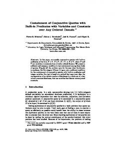
Approximation techniques can also be used to generate alternative forms of a query and search for answers in the data sources. For instance, tree-pattern query relaxation methods are presented in [4,5], while methods for producing approximate answers to XML queries are suggested in [15,30]. In the same direction, flexible and semiflexible semantics were introduced in [18] for tree and dag queries. Nevertheless, in all these cases the answer is not exact with respect to the initial query. Approaches based on keyword search [32,17,10,24] avoid the issue of unknown structure or the issue of multiple differently structured data sources since knowledge of the structure is not required for the queries. However, the total absence of structure has a number of drawbacks: (a) the user cannot specify structural information within the query to accelerate computation of the answer, (b) the user cannot impose structural conditions to filter out undesirable answers, and (c) the user cannot specify the structure of the query result. Some approaches aim at extending full-fledged XML query languages with keyword-based search techniques [13,23]. However, these languages are too complex for the simple user. Approaches with languages based on tree patterns share a restrictive feature: it is not possible in a tree pattern to indicate that two nodes n1 and n2 occur in a path without specifying a precedence relationship between them (node n1 has to precede node n2 or vice-versa). Such a restriction causes problems both to the formulation and processing of requests that do not specify an order among some nodes. Indeed, a number of tree-pattern queries that is exponential on the number of nodes of the query might need to be specified and processed. Our approach. To face the previous issues, we use a query language that allows partial specification of a tree structure. Consider the traditional tree-pattern queries shown in Figure 1. The nodes are labeled by elements. Annotations show value assignments to elements. For instance, the value of element SU BJECT is xml and the value of element Y EAR is 2006. Double line arrows denote descendant relationships, and single line arrows denote child relationships. A star (*) marks the output node (the node returned in the answer). Since the order of the elements in every root-to-leaf path of a tree pattern is fixed, the user might need to specify multiple alterna-

ART ICLE

AU T HOR∗ Y EAR = {2006}

ART ICLE

T IT LE

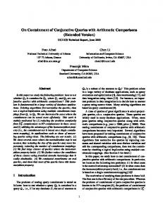
Fig. 2 A Partial Tree Pattern Query

tive queries if she cannot (or does not want to) specify an order among some elements. Three such alternative treepattern queries are shown in Figure 1. Consider now Figure 2. It shows a tree-pattern query where the tree structure is partially specified. This query has three “paths”. The first path involves elements SU BJECT and Y EAR, and Y EAR is a descendant of SU BJECT . The second path involves elements SU BJECT and ART ICLE, and no order is specified between them. The third path involves elements ART ICLE, T IT LE and AU T HOR. Element T IT LE is a child of ART ICLE, but AU T HOR can be an ancestor of ART ICLE or a descendant of T IT LE. The first and the second paths have a common element SU BJECT , while the second and the third paths have a common element ART ICLE. This is denoted by an edge labeled by ‘≡’. With this same query, we can retrieve the desired information from different tree structures that categorize publications by subject but also by article or author. We can also retrieve information when the structure is not fully known. This type of queries was initially introduced in [33], and are called partially specified tree-pattern queries (frequently mentioned simply as queries in the following). Their structure can be specified fully, partially or not at all. This flexibility allows their use for dealing efficiently with the issues mentioned above.

The problem. For a query language to be useful, it needs to be complemented with query processing and optimization techniques. Important issues in query optimization, including query satisfiability [22], query minimization [3,36,31], and query rewriting using views [28, 21], require solving the query containment problem. In this paper, we address query containment for partially specified tree-pattern queries in the presence of structural summaries of the data. The query containment problem has been studied in the past for (fully specified) tree-pattern queries in the absence and in the presence of constraints. Most of the previous work focuses almost exclusively on characterizing the complexity of the problem for tree patterns. Our goal here is to provide efficient (sound but not necessarily complete) methods for checking query containment in the presence of structural sum-


maries of data that can be used for processing partially specified tree-pattern queries. Contribution. We represent tree-structured data by considering trees of values whose nodes are partitioned to form what we call dimensions. Partial tree-pattern queries are specified on dimensions annotated with values, and are not cast on the structure of a specific value tree. The dimensions are used to define dimension graphs, a construct that summarizes the structural information of the value trees. The dimension graphs can be automatically extracted from value trees and support the processing and evaluation of the queries. Using a dimension graph G we can identify for each partially specified treepattern query Q a set of (fully specified) tree-pattern queries that are “equivalent” to Q in that they can be used to compute the answer of Q on any value tree underlying G. We call these fully specified queries dimension trees. The main contributions of this paper are the following: • We define the problem of partial tree-pattern query containment with respect to a dimension graph. • In order to allow query comparison we define a “normal form” for queries, called full form. Intuitively, a full form of a query comprises all the structural expressions and dimension annotations (value predicates) that can be derived from those specified in the query. • We identify connected sets of (partial) paths that can be added to or removed from any query without affecting its answer on any value tree. We call such sets of paths valid path clusters and we provide necessary and sufficient conditions for their complete characterization. • We provide necessary and sufficient conditions for query containment with respect to a dimension graph in terms of homomorphisms between the dimension trees of the queries. To support heuristic techniques, we also provide necessary but not sufficient conditions for query containment with respect to a dimension graph in terms of homomorphisms between queries. • In order to deal with the high complexity of query containment, we design two sound but not complete heuristic techniques based on structural expressions extracted from the dimension graph. The one heuristic technique computes and stores the structural expressions in advance, while the other computes the structural expressions on-the-fly (at query time). • We have implemented all the containment checking approaches mentioned above. We performed an extensive experimental evaluation to compare the pros and cons of every approach. Our experiments show that the heuristic approaches are efficient compared to non-heuristic ones while maintaining high accuracy. These results show that these techniques can be

3

directly exploited for partially specified tree-pattern query processing and optimization. Outline. The next section reviews related work. Section 3 presents the data model and the query language. Section 4 provides formal definitions and preliminary results. In Section 5, we present conditions for query containment. Section 6 introduces the heuristic approaches. Experimental results are shown in Section 7. We conclude in Section 8 and discuss future work. Proofs of propositions that are not difficult are omitted. 2 Related Work In this paper, we focus on checking query containment in the presence of dimension graphs. Dimension graphs are summaries of tree-structured data. Similar concepts have been referred to with different names in the literature, including “index graphs”, “path summaries”, “path indexes” and “structural summaries”. They differ in the equivalence relations they employ to partition the nodes of the data tree, which includes simulation and bisimulation [26,19]. Here, the nodes in the data tree are partitioned based on semantic relations provided by the user. This consideration is general and encompasses syntactic partitionings. For instance, in an XML tree, the equivalence classes can be formed by all the nodes labeled by the same element. Summaries of data have been extensively studied in recent years in both the “exact” [14, 26,29,6] and the “approximate” flavor [20,19]. A common characteristic of those approaches is that the data summary is used as a back end for evaluating a class of path expressions without accessing the data tree. To this end, the equivalence classes of nodes are attached to the corresponding nodes of the data summary. In contrast to previous approaches, here, the equivalence classes of the data tree nodes are not kept with the dimension graph. Therefore, partially specified tree-pattern queries are ultimately evaluated on the data tree. The dimension graphs are used to support the evaluation of the queries and the satisfiability and containment checking. Because of their importance for query processing, a considerable amount of work has focused on the satisfiability [16,22], containment [11,18,25,37,27,12,8] and minimization problems [3,31] for tree-pattern queries in the presence and in the absence of schemas. In particular, Neven and Schwentick [27] studied the complexity of tree pattern queries (involving child and descendant relationships and wildcards) in the presence of disjunction and DTDs. As we show later in the paper, using a dimension graph, a partially specified tree-pattern query can be expressed as a set of tree-pattern queries. However, the containment problem addressed in [27] is different than that of partially specified tree-pattern queries in the presence of dimension graphs because: (a) the semantics of dimension graphs is different than this of DTDs, and (b) not every set of tree pattern-queries can be expressed

4

as a partially specified tree-pattern query. Benedikt and Fundulaki [7] study query composition for different fragments of XPath under subquery semantics. None of these papers addresses query containment for partially specified tree-pattern queries. Most of the aforementioned works focus on studying the complexity of these problems for different classes of tree-pattern queries. Our goal in this paper is different. We are focusing on providing heuristic techniques for checking query containment in the presence of dimension graphs that can be used for efficiently processing and optimizing partial tree-pattern queries. Partially specified tree-pattern queries were initially introduced in [33], where inference rules were also provided to completely characterize the inference of structural expressions. Initial results on the query containment problem for partial tree-pattern queries were presented in [34,35]. In both of these papers the class of partial tree-pattern queries considered is restricted to disallow cases of unordered node sharing expressions between two or three partial paths. Further, the focus of [34] was not on heuristic approaches for query containment in the presence of dimension graphs. The data model in [35] is restricted not to allow values. Consequently, the query language does not involve value predicates, and new structural expressions cannot be derived from the interaction of existing structural expressions and value predicates. The present paper is the first one to consider a data model and query language for partial tree-pattern queries that is general enough to encompasses previous cases. It addresses the partial tree-pattern query containment problem in the presence of dimension graphs in a concise way and presents both necessary and sufficient conditions along with elaborate (sound but not complete) heuristic approaches for this problem. 3 Data Model and Query Language We present in this section our data model and query language. The data model represents tree-structured data using the concepts of value tree, dimension and dimension graph. The query language allows for partially specified tree patterns. 3.1 Value Trees and Dimension Graphs We assume an infinite set of values V that includes a special value r. Dimensions and value trees. A dimension set over V is a partition D of V that includes the singleton {r}. Each element of D is called dimension of D. The dimensions in D are assigned distinct names. In particular, the dimension {r} is named R. Intuitively, a dimension is a set of semantically related values. For instance, SU BJECT can be a dimension that includes values xml, databases


and data integration. Since the names of the dimensions are distinct we use them to identify the dimensions of D. Different applications may require and apply different partitions of the values in V . For the needs of this paper, we assume that a dimension set is fixed and we denote it by D. Definition 1 A value tree over D is a rooted node-labeled tree T , such that: (a) each node label in T belongs to V , (b) value r labels only the root of T , and (c) there are no two nodes on a path in T labeled by values that belong to the same dimension in D. In this sense, value trees are not recursive. ! We assume that nodes in a value tree have a unique node identifier and these node identifiers are preserved in the answers of a query on this value tree. Example 1 Let D = {R, A, B, C, D, E}. This will also be the dimension set for the rest of the examples in this paper. Figures 3 and 4 show two value trees T1 and T2 respectively. All the xi s in a value tree denote (not necessarily distinct) values of the same dimension X ∈ D. For instance, values a1 and a2 are values of dimension A. The numbers by the nodes of the value tree T2 of Figure 4 denote their identifiers. Values from two different dimensions can appear in different order in different branches of a value tree. For instance, value c1 of dimension C is an ancestor of value a1 of dimension A in the leftmost branch of tree T1 , while value c2 of dimension C is a descendant of value a2 of dimension A in another branch of T1 . ! The semantic interpretation of the values of a value tree into dimensions is provided by a user, possibly assisted by an ontology. Note, however, that dimensions can also be chosen to represent purely syntactic objects. For instance, they can be viewed as sets that group together nodes in the value tree that are labeled by the same element. In this case, the concept of a dimension graph is similar to that of an index graph [18]. Dimension graphs. The values of some dimension may not be children or descendants of any value of some other dimension in a value tree. For instance, no value of dimension A in the value trees T1 and T2 of Figures 3 and 4 is a child of a value of a dimension other than E. We use the concept of dimension graph to capture this type of relationship between dimensions in a value tree. Definition 2 Let T be a value tree over D. A dimension graph of T is a graph (N, E), where N is a set of nodes and E is a set of edges, defined as follows: (a) there is a node D in N if and only if there is a value in T that belongs to dimension D, and (b) there is a directed edge (Di , Dj ) in E if and only if there are nodes ni and nj in T labeled by values vi ∈ Di and vj ∈ Dj respectively, such that nj is a child of ni in T . If G is a dimension graph of a value tree T , we say that T underlies G. !


r

r

c1

c3

c1

e2

e1

e1

e2

a1

a1

a2 d2

d1

c2 b 2

b1

b1 d1

Fig. 3 Value tree T1

5

e2

0

1

R

8 9

2

a2

10

d3

3

4

b1

11

b2

6

5

7 d2

12

c1

Fig. 4 Value tree T2

The dimension graph of a value tree may have cycles. In particular, it can have a trivial cycle if, in the underlying value tree, a value of a dimension labels a parent node of a node labeled by a value of another dimension and conversely. Example 2 Figure 5 shows the dimension graph of the value trees T1 and T2 of Figures 3 and 4. Trivial cycles are shown in the figures with a double headed edge (e.g. the edge between dimensions D and B in Figure 5). ! The following proposition provides properties that fully characterize dimension graphs on value trees. Proposition 1 A directed graph G whose nodes are dimensions is a dimension graph of some value tree if and only if the following properties hold: (a) Graph G does not have disconnected components. (b) There is exactly one node in G having only outgoing edges. We call this node root of G. (c) For every directed edge in G there is a path1 from the root of G that comprises this edge. !

C B

E

D

A

Fig. 5 Dimension graph G

that the evaluation of a query on a value tree yields a value tree. Syntax. A query on a dimension set provides a (possibly partial) specification of a tree of dimensions annotated with sets of values. The tree is rooted at dimension R. A query specifies such a tree through a set of (possibly partially specified) paths from the root of the tree. For succinctness, in the following, PSP stands for partially specified path. Each PSP is defined in a query by a set of annotated dimensions, and a set of precedence relationships (child and descendant relationships) among these annotated dimensions. A query further indicates nodes (annotated dimensions) that are shared among different PSPs in the query tree. It also identifies a distinguished PSP called output PSP. The formal definition follows.

Definition 3 A query on a dimension set D is a triple (P, S, o), where: (a) P is a nonempty set of triples (p, A, R), where A and R define a PSP as explained below, and p is a distinct name for this PSP. Since PSP names are distinct, we identify PSPs with their names. (a1) A is a set of expressions of the form D[p] = V , Proof The only if part is straightforward. For the if part where D[p] denotes the dimension D of D in let’s assume that a directed graph G satisfies the condiPSP p, and V is a set of values of dimension tions (a), (b), and (c) of the proposition. We construct D or a question mark (“?”). These expressions a value tree by considering all the simple paths from the are called annotating expressions of p. If the root of G and by merging their root node R. Clearly, expression D[p] = V belongs to A we say that this tree is a value tree that underlies G. Therefore, G is D is annotated in p and V is its annotation. a dimension graph. ! A dimension can be annotated only once in a Dimension graphs can be automatically extracted from PSP p. Without mentioning it explicitly, we value trees and abstract their structural information. As assume that dimension R is annotated with a we show in subsequent sections, they help the evaluation “?” in every PSP. Set A can be empty. of queries on value trees, the detection of unsatisfiable (a2) R is a set of expressions of the form Di [p] → queries and the checking of query containment. Dj [p] or Di [p] ⇒ Dj [p], where Di is an annotated dimension in A or R, and Dj is an annotated dimension in A. These expressions are called precedence relationships of p. Set R 3.2 Query Language can be empty. Queries are issued on dimension sets and are evaluated (b) S is a set of expressions of the form D[pi ] ≡ D[pj ], where pi and pj are PSPs in P, and D is a dimenon value trees. Dimension graphs can support the formusion annotated in pi and pj . These expressions are lation of queries. To allow query composition, we require called node sharing expressions. Roughly speaking, 1 they state that PSPs pi and pj have a dimension in Paths here are meant to be simple that is, they do not meet the same node twice common. Set S can be empty.

6


(c) o is the name of one of the PSPs in P. This PSP is called output PSP of the query. ! The term structural expression refers indiscreetly to a precedence relationship or to a node sharing expression. Example 3 Consider the following query on D: Q1 = (P, S, p1 ), where P = {(p1 , A1 , R1 ), (p2 , A2 , R2 ), (p3 , A3 , R3 )}, A1 = {A[p1 ] =?, B[p1 ] = {b1 }, C[p1 ] = {c1 }, D[p1 ] =?}, R1 = {A[p1 ] ⇒ B[p1 ]} A2 = {A[p2 ] = ?, C[p2 ] = {c1 , c2 }, E[p2 ] = ?}, R2 = {C[p2 ] ⇒ A[p2 ], E[p2 ] → A[p2 ]} A3 = {C[p3 ] = ?, D[p3 ] = ?}, R3 = {D[p3 ] ⇒ C[p3 ]}, and ! S = {C[p1 ] ≡ C[p2 ]}.

Definition 4 Let T be a value tree over a dimension set D, and Q be a query on D. An embedding of Q into T is a mapping M of the annotated dimensions of the PSPs of Q to nodes in T such that: (a) The annotated dimensions of a PSP in Q are mapped to nodes in T that are on the same path from the root of T . (b) For every annotating expression D[p] = V in Q, the label of M (D[p]) is a value in V , if V is a set, and it is a value of D, if V is a “?”. (c) For every precedence relationship Dj [p] → Dk [p] (resp. Dj [p] ⇒ Dk [p]) in Q, M (Dk [p]) is a child (resp. descendant) of M (Dj [p]) in T . (d) For every node sharing expression D[pi ] ≡ D[pj ] in ! Q, M (D[pi ]) and M (D[pj ]) coincide.

A query can have more than one embedding into a We graphically represent queries using graph notation. Consider a query Q. Each PSP of Q is represented value tree. Given an embedding M of a query Q into as a (not necessarily connected) graph of dimensions la- a value tree T , and a PSP p in Q, the path from the beled by their annotating expressions in the PSP. The root of T that comprises all the images of the annotated name of each PSP is shown below the corresponding dimensions of p under M and ends in one of them is PSP graph. In particular, the name of the output PSP called image of p under M and is denoted M (p). Notice of Q is preceded by a !. PSP names are omitted in the that more than one PSP of Q may have their image in annotating expressions for succinctness. Child and de- the same root-to-leaf path of T (M does not have to be scendant precedence relationships in a PSP are depicted a bijection). using single (→) and double (⇒) arrows between the re- Definition 5 Let T be a value tree over a dimension set spective nodes in the PSP graph. Two nodes (annotated D, and Q = (P, S, o) be a query on D. The answer of Q dimensions) in different PSP graphs that participate in on T is a tree T ! such that: a node sharing expression of Q are linked in its graphical (a) T ! results by removing (possibly 0) paths from T . representation with a straight line labeled by the symbol (b) For every embedding of Q into T , the image of the ‘≡’. output PSP of Q is in T ! . (c) Every root-to-leaf path of T ! is the image of the outExample 4 Query Q1 of Example 3 is graphically repreput PSP of Q under an embedding of Q into T . sented in Figure 6. The graphical representation of other If there is no such a tree T ! , the answer of Q on T is queries is shown in Figures 8 and 9. ! an empty tree, and we say that the answer of Q on T is empty. ! C = {c1 }

≡

C = {c1 , c2 }

D =?

E=?

A=?

D=?

A=?

C=?

B = {b1 } PSP ∗p1

PSP p2

PSP p3

Fig. 6 Query Q1

Semantics. The answer of a query Q on a value tree T is a value tree. Every path from the root to a leaf of the answer of Q on T is the image of the output path of Q under an embedding of Q into T that preserves the precedence relationships and node sharing expressions of Q. Note that the answer of a query is defined here differently than in XPath where the answer of an expression is a set of nodes.

Note that annotating a dimension with a “?” in a PSP of a query is different than omitting this dimension from the PSP. A dimension of a PSP that is annotated with a “?” requires one of its values to be in the image of the PSP under every query embedding into the value tree. Example 5 Consider the query Q1 of Example 3, graphically shown in Figure 6. Consider also the value tree T2 of Figure 4. The answer of Q1 on T2 is shown in Figure 7. There are two embeddings of Q1 into T2 which result in two distinct root-to-leaf paths in the answer of Q1 on T2 . The embeddings are as follows: Embedding 1: C[p1 ] → 1, A[p1 ] → 3, B[p1 ] → 5, D[p1 ] → 4, C[p2 ] → 1, E[p2 ] → 2, A[p2 ] → 3, D[p3 ] → 10, C[p3 ] → 12. Embedding 2: C[p1 ] → 1, A[p1 ] → 3, B[p1 ] → 6, D[p1 ] → 7, C[p2 ] → 1, E[p2 ] → 2, A[p2 ] → 3, D[p3 ] → 10, C[p3 ] → 12. Note that both embeddings map the dimensions of PSPs p1 and p2 of Q1 to nodes on the same path from the root of T2 . !

Containment of Partially Specified Tree-Pattern Queries in the Presence of Dimension Graphs C = {c1 }

r c1

D=? A=?

e1 a1

B = {b1 }

d1

b1

b1

d2

PSP ∗p7 Fig. 9 Query Q3

Fig. 7 The answer of Q1 on T2

4 Problem Definition and Preliminary Results We define in this section query containment and we provide concepts and preliminary results that will allow us to study the problem of checking two queries for containment. 4.1 Query Containment Queries are to be evaluated on value trees that underlie a specific dimension graph. Even though dimension graphs are not schemas in the sense of e.g. a DTD of an XML document, we use them as schemas in processing and evaluating queries. Therefore, we define query containment and equivalence with respect to a dimension graph. Definition 6 Let Q1 and Q2 be two queries on D, and G be a dimension graph on D. Query Q1 contains query Q2 with respect to dimension graph G (denoted Q2 ⊆G Q1 ) if and only if for every value tree T over D underlying G, every root-to-leaf path in the answer of Q2 on T is also a root-to-leaf path in the answer of Q1 on T . Queries Q1 and Q2 on D are equivalent with respect to dimension graph G (denoted Q2 ≡G Q1 ) if and only if Q1 ⊆G Q2 and Q2 ⊆G Q1 . ! Example 6 Consider the queries Q1 , Q2 and Q3 shown in Figures 6, 8 and 9 respectively. Consider also the C = {c1 }

A=?

≡

C = {c1 , c2 }

D=?

D=?

≡

B = {b1 , b2 } PSP p4 Fig. 8 Query Q2

7

B = {b1 , b3 } PSP ∗p5

E=? A=? PSP p6

dimension graph G of Figure 5. One can see that Q1 ⊆G Q2 , and Q2 ⊆G Q3 . Further, Q3 ⊆G Q2 , and therefore

Q2 ≡G Q3 . In contrast, Q2 '⊆G Q1 . We will prove these claims in Section 5. ! 4.2 Structural Expression Inference and Query Full Form Because tree patterns are partially specified in the queries, new, non-trivial expressions (structural expressions but also annotating expressions) can be inferred from those explicitly specified in the queries. These expressions are preserved by all the embeddings of the query to a value tree; in other words, adding these expressions to the query does not remove paths from its answer on any value tree. We formalize below the notion of structural expression implication. Definition 7 Let E be the set of expressions of a query Q on a dimension set D, and e be an expression. We say that e is implied from E (denoted E |= e) if and only if for every value tree T over D and every embedding M of Q into T , M preserves e. ! Example 7 Consider the set of structural expressions E = {A[p1 ] ⇒ B[p1 ], A[p1 ] ≡ A[p2 ], R[p2 ] ⇒ B[p2 ]}. One can see that E implies the precedence relationship A[p2 ] ⇒ B[p2 ]. ! The closure of a set E of expressions is the set that includes the expressions in E and those structural expressions that can be implied from E. In order to check queries for containment, we introduce a “normal form” for queries called full form. A query is in full form if its set of expressions E is closed under implication (that is, E equals the closure of E). Note that we ignore in E an annotating expression D[p] = V , if a more restrictive annotating expression D[p] = V ! , with V ! ⊆ V , also belongs to E. Clearly, a query can be equivalently put in full form by replacing its set E of expressions by the closure of E. To graphically represent queries in full form, we follow the following convention: (a) double arrows (ancestor precedence relationships) from R are not depicted, (b) a double arrow between two dimensions in a PSP is not

8


depicted if it can be transitively derived from other double arrows in the same PSP, and (c) a double arrow from dimension D1 to dimension D2 in a PSP is not depicted if there is a single arrow from D1 to D2 in the same PSP. All the omitted double arrows and node sharing expressions can be trivially derived from the expressions explicitly represented in the query graph. Example 8 Consider the queries Q1 and Q2 of Figures 6 and 8. Figures 10 and 11 show the full form of Q1 and Q2 respectively. Query Q3 of Figure 9 is in full form. ! C = {c1 }

C = {c1 }

≡

A=?

D=?

E=?

D=?

C=?

B = {b1 }

A=?

PSP ∗p1

PSP p2

PSP p3

Fig. 10 Full form of Query Q1

C = {c1 }

≡

A=? D=?

B = {b1 } PSP p4

≡

≡

C = {c1 }

≡

C = {c1 }

A=? A=? D=? B = {b1 }

E=?

PSP ∗p5

PSP p6

Fig. 11 Full form of Query Q2

A set of inference rules for structural expression implication has been provided in [35]. Each inference rule derives a new structural expression from a set of structural expressions. For instance, the following inference rule derives a descendant precedence relationship: a[p1 ] → b[p1 ], c[p2 ] → b[p2 ], d[p1 ] ≡ d[p2 ] ( d[p1 ] ⇒ a[p1 ], where a, b, c and d are dimensions and p1 and p2 are PSPs. Clearly, the number of structural expressions that can be derived using the inference rules in a query is bound by O(n2 ), where n is the product of the distinct dimensions in the query and its number of PSPs. Therefore, the full form of a query can be computed in polynomial time.

4.3 Unsatisfiable Queries and Valid PSP Clusters Similarly to query containment, we define query unsatisfiability in the presence of a dimension graph. Definition 8 Let G be a dimension graph on D. A query on D is unsatisfiable with respect to G if its answer is empty on every value tree underlying G. Otherwise, it is called satisfiable with respect to G. ! An unsatisfiable query is contained in any query with respect to a dimension graph. In [33], necessary and sufficient conditions are provided for query unsatisfiability. In the following we assume that queries are satisfiable with respect to G. A set of PSPs in a query that are all linked together through node sharing expressions is called cluster: Definition 9 A cluster is a set C of PSPs and node sharing expressions such that for every partition of C in two non-empty sets there is a node sharing expression in Q on an element different than R involving PSPs from both sets (that is, the cluster does not comprise disconnected sets of PSPs). ! We represent clusters as queries without an output PSP (see, for instance, Figures 12 and 13). Given a dimension graph G, it is possible that there is a cluster that can be added to any query without affecting its answer on any value tree that underlies G. To deal with this issue, we introduce the concept of valid cluster. Definition 10 Let G be a dimension graph on D. A cluster Q is valid with respect to G if and only if, for every value tree T over D underlying G, there is a mapping M of the annotated dimensions of Q to nodes of T that satisfies the conditions (a), (b), (c) and (d) of definition 4 (i.e., M is an embedding of Q into T ). ! Example 9 Consider the dimension graph G of Figure 5. Let C1 be the cluster that consists of a single PSP comprising a single dimension A annotated with a ‘?’. Since A appears in G, C1 is valid. Let also C2 be the cluster that consists of a single PSP p2 comprising two dimensions C and E annotated with a “?” and a child precedence relationship C → E. Since there is an edge (C, E) in G, it is not difficult to see that C2 is valid with respect to G. Valid clusters can involve several PSPs. Consider the clusters C3 and C4 shown in Figures 12 and 13. As it will become clear below, these clusters are valid with respect to G. ! Clearly, adding to a query Q a valid cluster or removing from a query a valid cluster that does not include the output PSP of Q and does not share nodes with paths outside the cluster results in a query equivalent to Q. One can see that the only way for a cluster to be valid is that the embedding of Definition 10 maps every PSP in

Containment of Partially Specified Tree-Pattern Queries in the Presence of Dimension Graphs A=?

E=? A=?

≡

B=?

≡

PSP p1

B=?

PSP p2

Fig. 12 Cluster C3 (valid) E=?

E=?

A=?

≡

E=?

A=? D=?

D=?

B=?

≡

PSP p1

PSP p2

PSP p3

Fig. 13 Cluster C4 (valid)

the cluster to the same path in the value tree T . The following proposition exploits this observation to provide necessary and sufficient conditions for a cluster to be valid with respect to a dimension graph. Proposition 2 Let G be a dimension graph on D and C be a cluster on D. Cluster C is valid with respect to G if and only if the following conditions hold: (a) Every dimension in C is annotated with a “?” (or with the set of all the values of the dimension), and (b) There is an edge in G such that for every path p from the root of G that comprises this edge there is a mapping from the annotated dimensions in C to the dimensions of p that preserves the dimensions and all the precedence relationships in C. ! Proof: (If part) Let’s assume that cluster C is valid and condition (a) does not hold. Then, there is a dimension D in C, which is not annotated with a “?” (or with the set of all the values of the dimension). This means there is d ∈ D that is not in the annotation of D in at least one PSP p of C. We construct a value tree T underlying G such that d is the only value of dimension D in T . Clearly, PSP p does not have an embedding to T . This contradicts our assumption that cluster C is valid. Let’s now assume that cluster C is valid and condition (b) does not hold. Then, there is no edge such that for every path p from the root of G that comprises this edge there is a mapping from C to p preserving dimensions and precedence relationships. We construct a tree T as follows: Start with an empty value tree T . For each edge e in dimension graph G find a path p from the root of G containing e such that there is no embedding from

9

cluster C into p. For each path p add a root-to-leaf path to T constructed from p by replacing labeling dimension by one of their values. These paths in T have a single common node labeled by r. Clearly, T is a value tree underlying graph G. Further, by construction, there is no embedding of C into T that maps all PSPs of C into the same path of T . Since the paths of T do not share nodes (other than the root node) and all the PSPs of C are involved in node sharing expressions, there is no embedding of C into T . This contradicts our assumption that cluster C is valid. (Only if part) Let’s assume that conditions (a) and (b) hold, and let T be a value tree underlying G. Consider an edge e = (Di , Dj ) in G satisfying condition (b). By Definition 2, in every value tree T underlying G, there are nodes ni and nj in T labeled by values vi ∈ Di and vj ∈ Dj , respectively, such that nj is a child of ni . Let p! = r, n1 , . . . , nk , ni , nj be a path in T where nl ∈ Dl , l in [1, k] ∪ {i, j}, and p be the path R, D1 , . . . , Dk , Di , Dj in G. Since p contains e, there is a mapping from C to p that preserves dimensions and precedence relationships in C. Therefore, there is a mapping m from C to p! that preserves dimensions and precedence relationships. Since condition (a) holds, all the dimensions in C are annotated by “?” and therefore m is an embedding of C into p! . Thus, C can be embedded to any value tree underlying G, that is, it is valid wrt G. !

Example 10 Consider the cluster C3 of Example 9 shown in Figure 12. There are two paths from the root of G that comprise edge (A, B). Each path involves all the annotated dimensions in C3 and satisfies the precedence relationships of both PSPs of C3 . Therefore, cluster C3 is valid. Consider also the cluster C4 of Example 9 shown in Figure 13. As before, we can show that there are exactly two paths from the root of G that comprise edge (D, B) and each of them involves all the annotated dimensions in C4 and satisfies the precedence relationships of all ! three PSPs of C4 . Therefore, C4 is also valid. Checking for valid clusters can be performed efficiently as the next proposition shows. Proposition 3 Let G be a dimension graph on D, and C be a cluster on D. Let also n be the product of the number of dimensions in G and the number of PSPs in C. Checking if C is valid with respect to G can be done in polynomial time on n. !

Proof: (Sketch) Based on Proposition 2, checking if C is valid can be performed as follows: (a) for every edge (X, Y ) in G, compute the set of precedence relationships that hold on every path from the root of G that comprises (X, Y ), and (b) check if some of these sets contains all the precedence relationships of C. If this is the case, C is valid with respect to G. The set S of descendant precedence relationships that hold on every path from the root of G that comprises (X, Y ) can be computed as follows:

10

(a) Initially let S = {X ⇒ Y }. (b) Remove every outgoing edge from Y in G to create a new graph G ! . (c) For every node Z, Z '= X, Z '= Y of G ! , remove all the outgoing edges from Z, and check if there is no path from the root of G ! to X. If this is the case, add Z ⇒ X to S. (d) For every precedence relationship Z ⇒ X added to S in step (c), apply recursively step (c) to node Z. The set S ! of child precedence relationships that hold on every path from the root of G that comprises (X, Y ) can be computed from S as follows: initially let S ! = {X → Y }. For every V ⇒ W ∈ S, if V → W appears in G ! , remove it and check if there is no path from the root of G ! to X. If this is the case, add V → W to S ! . Since there are at most m2 edges in G, where m is the number of nodes of G, and checking the existence of a path between the root of G and a node can be done in O(m2 ), the previous process can be done in polynomial time on m. Since the number of precedence relationships in C is O(n), where n is the product of the number of nodes in G and the number of PSPs in C, checking the validity of C can be done in polynomial time on n. ! In the following, we assume that a query does not comprise a valid disconnected cluster that does not contain the output PSP of the query. 5 Checking Query Containment With Respect to a Dimension Graph In order to address query containment with respect to a dimension graph, we need the concept of homomorphism between partially specified tree-pattern queries. Definition 11 Let Q1 and Q2 be two queries on D. A homomorphism from Q2 to Q1 is a mapping h from the annotated dimensions of Q2 to the annotated dimensions of Q1 such that: (a) If the annotated dimension n is labeled by a dimension D in Q2 , then h(n) is also labeled by D in Q1 . (b) All the annotated dimensions of a PSP in Q2 are mapped under h to annotated dimensions in the same PSP of Q1 . (c) If an annotated dimension n in Q2 is annotated by V2 '=?, then h(n) in Q1 is annotated by V1 such that V1 ⊆ V2 . (d) The annotated dimensions in the output PSP o2 of Q2 are mapped under h to annotated dimensions in the output PSP o1 of Q1 , and every annotated dimension in o1 is the image under h of an annotated dimension in o2 . (e) If D[p] → D! [p] (resp. D[p] ⇒ D! [p]) is in Q2 , then h(D[p]) → h(D! [p]) (resp. h(D[p]) ⇒ h(D! [p])) is in Q1 . (f) If D[p] ≡ D[p! ] is in Q2 , then h(D[p]) and h(D[p! ]) coincide or h(D[p]) ≡ h(D[p! ]) is in Q1 . !


The existence of a homomorphism between queries is a sufficient condition for query containment with respect to a dimension graph as the next proposition shows. Proposition 4 Let Q1 and Q2 be two queries on D, where Q1 is in full form, and G be dimension graph. If there is a homomorphism from Q2 to Q1 , then Q1 ⊆G Q2 . ! Proof: Let M be an embedding of Q1 into a value tree T underlying G, and h be a homomorphism from Q2 to Q1 . Clearly, the composition of M on h, M ◦ h, is an embedding of Q2 into T . Therefore, Q1 ⊆G Q2 . !

Example 11 Let Q!1 be the query shown in Figure 10. This is the full form of query Q1 of Figure 6. Consider also query Q2 shown in Figure 8. One can see that there is a homomorphism from Q2 to Q!1 . Therefore, ! Q1 ⊆G Q2 .

Unfortunately, the existence of a homomorphism is not a necessary condition for query containment with respect to a dimension graph. Example 12 Consider, queries Q2 and Q3 of Figures 8 and 9, respectively. Query Q3 is in full form. As mentioned in Example 6, Q3 ⊆G Q2 . However, there is no homomorphism from Q2 to Q3 since dimension E of Q2 does not appear in Q3 . ! In order to fully characterize query containment with respect to a dimension graph, we use the concept of dimension tree of a query on a dimension graph. Definition 12 Let Q be a query on a dimension set D, and G be a dimension graph on D. Let also Q! be the full form of Q. A dimension tree of Q on G is a tree U such that: (a) The nodes of U are labeled by dimensions in D and their annotations (annotating expressions). No two nodes on a path of U are labeled by the same dimension. (b) One of the nodes of U is marked. This node is called output node of U , and the path from the root to the output node of U is called output path of U . (c) There is a mapping m from the set of the nodes of U to the set of nodes of G such that: (c1) If n is a node of U , n and m(n) are labeled by the same dimension. (c2) If (n1 , n2 ) is an edge in U , (m(n1 ), m(n2 )) is an edge of G. (d) There is a mapping m! from the set of the annotated dimensions of Q! to the set of nodes of U such that: (d1) The annotated dimensions of a PSP in Q! are mapped under m! to nodes on the same path of U . (d2) The marked node of U is the image under m! of an annotated dimension of the output PSP o of Q! that is the descendant in U of the images under m! of all the other annotated dimensions of o.


(d3) For every precedence relationship A[p] → B[p] (resp. A[p] ⇒ B[p]) in Q! , m! (B[p]) is a child (resp. descendant) of m! (A[p]) in U . (d4) If a node sharing expression D[p1 ] ≡ D[p2 ] is in Q! , m! (D[p1 ]) = m! (D[p2 ]). (d5) A dimension D of Q! annotated by V is mapped by m! to a node n labeled by D and annotated by V . (d6) Every leaf node in U is the image under m! of an annotated dimension of Q! . (d7) For a dimension D in PSPs p1 and p2 in Q, m! (D[p1 ]) '= m! (D[p2 ]) unless D[p1 ] ≡ D[p2 ] ! is in Q! . Intuitively, a dimension tree for Q on G represents a mapping of Q into G that respects PSPs, labeling dimensions, precedence relationships, and node sharing expressions. This mapping is the composition m ◦ m! of m! and m. The dimensions trees of Q on G represent all such possible mappings of Q into G. Example 13 Consider query Q1 of Figure 6 on the dimension graph G of Figure 5. Figure 14 shows the diR

R

C = {c1 } E A

C = {c1 }

E E

A

A

D

A

B

D

B = {b1 }

C

D (a)

E

E E

A

A

D B

B = {b1 }

C

(b)

Therefore, the answer of Q on T can be constructed by merging into a single value tree the answers of the dimension trees of U on T . The identities of the nodes are used to perform this merging. We now state a theorem that provides necessary and sufficient conditions for relative query containment, in terms of homomorphisms between dimension trees. Theorem 1 Let Q1 and Q2 be two queries on D and G be a dimension graph on D. Let also U1 and U2 be the sets of dimension trees of Q1 and Q2 , respectively, on G. Q1 ⊆G Q2 if and only if there is a mapping f from U1 to U2 such that, for every dimension tree U in U1 , there is a homomorphism from f (U ) to U . ! Proof: We start by the if part. Let M be an embedding of a dimension tree U ∈ U1 into a value tree T that underlies G. Let h be an homomorphism from the dimension tree f (U ) ∈ U2 . The composition of h on M , h ◦ M , is an embedding of f (U ) on T . Therefore, Q1 ⊆G Q2 . For the only if part, let’s assume that Q1 ⊆G Q2 and there is no such mapping f from U1 to U2 . Then, there exists a dimension tree U1 in U1 such that there is no homomorphism from any dimension tree in U2 to U1 . We construct a value tree T by replacing in U1 each labeling dimension by one of its annotating values. Clearly, T underlies G. Since there is no homomorphism from a dimension tree U2 in U2 to U1 , no U2 can be embedded into T . Therefore, Q1 has an answer on T while the answer of Q2 on T is empty. This contradicts our assumption that Q1 ⊆G Q2 . ! Example 14 Consider the queries Q1 , Q2 and Q3 of Example 13, shown in Figures 6, 8, and 9, and the dimension graph G of Figure 5. Figures 14, 15, and 16 show the dimension trees of Q1 , Q2 , and Q3 on G, respectively.

Fig. 14 The dimension trees of Q1 on G: (a) U11 , (b) U12

R

R

C = {c1 }

C = {c1 }

mension trees of Q1 on G. For simplicity of presentation, dimension annotations that are ‘?’ are not shown in the graphical representation of dimension trees. ! A dimension tree of a query on a dimension graph can be seen as a query where the tree structure is completely specified: root-to-leaf paths determine PSPs; the output path determines the output PSP; edges determine child precedence relationships; common nodes of two paths determine node sharing expressions. Such queries form a tree pattern without missing edges involving only parentchild (and not ancestor-descendant) relationships. Since dimension trees are special cases of queries, we can apply to them the concepts defined on queries: answer of a query, and homomorphism between queries. Given a dimension graph G, a query Q is associated to the set U of its dimension trees on G. Every path in the answer of Q on a value tree T underlying G is also a path in the answer of some U ∈ U on T , and conversely.

11

E

E

E

E

A

A

A

A

B = {b1 } D (a)

D

D (b)

B = {b1 }


Theorem 1 proves the claim of Example 13 that Q1 ⊆G Q2 : let f be the mapping f (U11 ) = U21 and f (U12 ) = U22 . Clearly, there is a homomorphism h from the nodes of U21 to U11 and from U22 to U12 . Based on Theorem 1, we can also show that Q2 ⊆G Q3 and Q3 ⊆G Q2 . Theorem ! 1 also proves that, in contrast, Q2 '⊆G Q1 .

12

Dimitri Theodoratos et al. R

R C = {c1 }

C = {c1 }

E

E

A

A

B = {b1 } (a)

D D

(b)

B = {b1 }


is in full form) contains the dimension A. Therefore, if we add the extracted precedence relationship E ⇒ A to p7 we obtain a query which is equivalent to Q3 with respect to G. Similarly, one can see that the following rule instance holds on G: if a path from the root of G satisfies the precedence relationship R ⇒ D, it also satisfies the precedence relationships E ⇒ D and A ⇒ D. Therefore, we can again add to p7 the extracted precedence relationships E ⇒ D and A ⇒ D to obtain a query equivalent to Q3 with respect to G. Taking the full form of the resulting query Q!3 , we obtain the query shown in Figure 17. Query Q!3 has more precedence relationships than Q3 . It C = {c1 }

One can see that there can be a number of dimension trees for a given query Q and dimension graph G that is exponential on the number of nodes of G. However, if the dimension graph is a tree, query Q has a single dimension tree with respect to G.

A=? B = {b1 }

6 Heuristic Approaches for Query Containment with Respect to a Dimension Graph Fig. 17 Query

Checking query containment with respect to a dimension graph can be time consuming since, as we saw in the previous section, it involves checking the existence of homomorphisms between pairs of dimension trees (Theorem 1). As mentioned in the previous section, the number of these pairs can be very large. Therefore, we cannot rely on Theorem 1 for checking efficiently containment of partial tree-pattern queries. In this section, we suggest a heuristic approach for checking two queries for containment with respect to a dimension graph G that reduces to checking the existence of a homomorphism only between two queries. 6.1 The basic idea Suppose that we want to check if query Q is contained in query Q! with respect to G. If there is a homomorphism from Q! to the full form of Q, by Proposition 4, we deduce that Q ⊆G Q! . However, if such a homomorphism does not exist, Q might or might not be contained in Q! . As an example, consider queries Q2 and Q3 shown in Figures 8 and 9. Query Q3 is in full form. Consider also the dimension graph G of Figure 5. As mentioned in Example 12, there is no homomorphism from Q2 to Q3 . Therefore, we cannot, based on this fact, decide on the containment of Q3 in Q2 with respect to G. Observe now that the following statement holds on G: if a path from the root of G contains dimension A (that is, if it satisfies the precedence relationship R ⇒ A), it also satisfies the precedence relationship E ⇒ A. We call such a statement “rule instance” and the precedence relationship E ⇒ A is qualified as extracted. The PSP p7 of query Q3 (which

E=?

Q!3

D=? PSP ∗p7

is not difficult to see now that there is a homomorphism from Q2 to Q!3 . Since Q!3 is equivalent to Q2 with respect to G, we can deduce that Q3 ⊆G Q2 . Therefore, the basic idea is to extract precedence relationships from the dimension graph G that can be iteratively added to query Q to produce appropriately an equivalent query with respect to G (called augmented form of Q). The possibility for the existence of a homomorphism from query Q! to the augmented form of query Q is increased. If such a homomorphism exists we can deduce that Q ⊆G Q! . There are two ways to implement the heuristic approach. The first one (called precomputation heuristic approach) considers a rule instance pattern (called rule). It computes in advance and stores all the rule instances of this rule that hold on G. When a query Q emerges, the extracted precedence relationships of these rule instances are used to compute the augmented form of Q. Using multiple rules instead of one provides a more refined characterization of G, and increases the accuracy (completeness) of the approach. The possibility of missing the detection of a query containment case with respect to G is reduced. However, this gain in accuracy is obtained at the expense of the space required to store the rule instances that hold on G, and the overall time required to compute the augmented form of Q. Therefore, a trade-off should be determined between the desired accuracy and the space and time cost incurred by the multiple rules considered by the precomputation heuristic approach.


The second way to implement the heuristic approach (called on-the-fly heuristic approach) considers all the precedence relationships in a PSP of query Q in order to extract from G the precedence relationships that are used for computing the augmented form of Q. Therefore, the precedence relationships are extracted from the dimension graph at query time. We formally define below both heuristic approaches.

13

Definition 15 A rule instance PI =⇒ CI holds on a dimension graph G, if the precedence relationships in CI are satisfied by every path from the root of G that satisfies the precedence relationships in PI , and there is no rule instance PI =⇒ C ! I with the same property such that CI ⊂ C ! I . !

Example 15 Consider the rule {R ⇒ X} =⇒ {Y → X, Y ⇒ X}. One can see that the following instances of this rule hold on the dimension graph G of Figure 5: 6.2 Precomputation heuristic approach {R ⇒ A} =⇒ {R ⇒ A, E ⇒ A, E → A}, {R ⇒ B} =⇒ {R ⇒ B, A ⇒ B, E ⇒ B}, We first introduce the concept of precedence relationship {R ⇒ C} =⇒ {R ⇒ C}, extraction rule. {R ⇒ D} =⇒ {R ⇒ D, A ⇒ D, E ⇒ D}, {R ⇒ E} =⇒ {R ⇒ E}. In the case of dimensions C and E, no new precedence 6.2.1 Precedence relationship extraction rules relationships can be extracted from G by the respective ! Definition 13 A (precedence relationship extraction) rule rule instances. is an expression of the form P =⇒ C, where P and C are non-empty sets of precedence relationship types. A prece- 6.2.2 Adding precedence relationships to queries dence relationship type is a precedence relationship that involves dimension variables (instead of dimensions), and Given a query Q, precedence relationships extracted from (possibly) dimension R. ! a dimension graph G by rule instances that hold on G can be appropriately added to Q to create the augmented For example, {R ⇒ X} =⇒ {Y ⇒ X} is a rule, form of Q. where X and Y are dimension variables. Definition 16 Consider a query Q, a dimension graph Definition 14 An instance of a rule P =⇒ C is an ex- G and a rule R. The augmented form of Q with respect pression of the form PI =⇒ CI obtained as follows: let αI to G, and R, say Q! , is constructed from Q as follows: be an assignment of dimensions to the dimension vari- Let initially Q! = Q. ables occurring in P. Repeat the following steps until no more changes can be (a) PI , the premise, is the set of precedence relationships applied to Q! : obtained by assigning distinct dimensions to all the - Put Q! in full form. dimension variables in P according to αI , and - For every PSP p in Q! and for every instance (b) CI , the conclusion, is a set of precedence relationships PI =⇒ CI of R that holds on G, if the precedence where each of them is obtained from a precedence relationships in PI appear in p, add to p the precerelationship type in C by replacing in it: (i) every dence relationships in CI . ! variable X that occurs also in P by αI (X), and (ii) every variable Y that does not occur in P by some We can now state the following proposition. dimension. ! Proposition 5 Let Q be a query, G be a dimension graph, Note that as a consequence of the previous defini- and R be a rule. The augmented form of query Q with tion, a precedence relationship type in the conclusion of respect to G and R is a query equivalent to Q with respect ! a rule might contribute multiple precedence relationships to G. to the conclusion of an instance of this rule obtained ! of query Q with by replacing a dimension variable that does not appear Proof: Let Q be the augmented form ! respect to G and R. In constructing Q , whenever a precein the premise of the rule by multiple dimensions. It is dence relationship P is added to a PSP p of Q, there is also possible that a precedence relationship type in the an instance of R, R , such that R holds on G, all the I I conclusion of a rule does not contribute any precedence appear in precedence relationships in the premise of R I relationships to the conclusion of an instance of this rule. p, and P appears in the conclusion of R . Therefore, for I Consider, for instance, the dimension graph G of Figtree T , the image of ure 5. An instance of the rule {R ⇒ X} =⇒ {Y → X, every embedding of Q to a value ! p satisfies P . Consequently, Q ⊆ Q. Clearly, Q ⊆ Q! . Y ⇒ X} is {R ⇒ D} =⇒ {R ⇒ D, A ⇒ D, E ⇒ D}. ! ! Intuitively, the premise of this instance characterizes all Therefore, Q ≡ Q . the paths from the root of G that involve dimension D. Generating the augmented form of a query Q inThe conclusion comprises descendant precedence rela- volves adding repeatedly to it precedence relationships tionships to D. extracted from the dimension graph and computing the

14


full form of the resulting query until a fixed point is reached. Computing the full form of a query possibly adds structural expressions (precedence relationships and node sharing expressions) to it. This process increases the possibility for homomorphisms from other queries to Q to exist. Example 16 Consider queries Q2 and Q3 of Figures 8 and 9 and the dimension graph G of Figure 5. In Example 12, we showed that there is no homomorphism from Q2 to Q3 . Consider now the rule R : {X ⇒ Y } =⇒ {U ⇒ V }. Figure 18 shows query Q!3 , the augmented form of query Q3 with respect to G and R. Query Q3 and rule C = {c1 } E=?

6.2.3 Using multiple rules Using additional rules in the heuristic approach improves its accuracy. Example 17 Consider query Q!2 of Figure 19 (a slight variation of query Q2 of Figure 8). Consider also query C = {c1 }

A=?

≡

C = {c1 , c2 } E=?

D=?

D=?

≡

B = {b1 , b2 }

B = {b1 , b3 } PSP ∗p5

PSP p4 Fig. 19 Query

Q!2

A=? PSP p6

A=? B = {b1 }

Fig. 18 Query G and R

Q!3 ,

D=? PSP ∗p7

the augmented query Q3 with respect to

R are simple and therefore, one iteration is enough for computing Q!3 . Observe that Q!3 has more precedence relationships than Q3 . Clearly, there is a homomorphism from Q2 to Q!3 . By Proposition 5, Q!3 ≡G Q3 . Then, by Proposition 5, Q3 ⊆G Q2 . This result proves again what we showed in Example 14 using Theorem 1. !

Q3 of Figure 9, and the dimension graph G of Figure 5. Figure 18 shows query Q!3 , the augmented form of query Q3 with respect to G and rule R : {X ⇒ Y } =⇒ {U ⇒ V }. There is no homomorphism from Q!2 to Q!3 . Therefore, a heuristic approach that uses only R fails to detect that Q3 ⊆G Q!2 . Let’s assume now that the heuristic approach employs not only rule R but also rule R! : {X ⇒ Y } =⇒ {U → V }. Figure 20 shows query Q!!3 , the augmented form of query Q3 with respect to G and {R, R! }. Clearly, there is a homomorphism from Q!2 R=? C = {c1 }

The next proposition shows that if the dimension graph is a tree, a simple rule can guarantee total accuracy for the heuristic approach. Proposition 6 Let Q1 and Q2 be two queries in full form, G be a dimension graph which is a tree, and R be the rule {R ⇒ X} =⇒ {Y → X}. Let also Q!1 be the augmented form of query Q1 with respect to G and R. Then Q1 ⊆G Q2 if and only if there is a homomorphism ! from Q2 to Q!1 . Proof: If G is a tree, Q1 (resp. Q2 ) has a single dimension tree U1 (resp. U2 ) on G. Clearly, Q1 ≡G U1 . If there is a homomorphism from Q2 to Q!1 , then by Proposition 4, Q!1 ⊆G Q2 . Since G is a tree, Q!1 is equivalent to U1 . Since Q1 ≡G U1 , Q1 ⊆G Q2 . If Q1 ⊆G Q2 then, from Theorem 1, there is a homomorphism from U2 to U1 . Then, since Q!1 is equivalent to U1 , there is a homomorphism h from U2 to Q!1 . By definition 12, there is a mapping m! from the nodes of Q2 to those of U2 . The composition of m! on h, h ◦ m! , ! is a homomorphism of Q2 to Q!1 .

E=? A=? B = {b1 }

Fig. 20 Query G and {R, R! }

Q!!3 ,

D=? PSP ∗p7

the augmented query Q3 with respect to

to Q!!3 . Therefore, the heuristic approach that uses both rules succeeds in deducing that Q3 ⊆G Q!2 . !

The gains in accuracy are obtained at the expense of (a) additional time for determining the rule instances that hold on G, (b) extra space for storing those rule instances, and (c) additional time for computing the augmented form of the query (possibly more rule instances


to be checked for application, more precedence relationships to be added to the query, and more iterations in the computation of the augmented form of the query). These drawbacks can be alleviated if we use a sequence of rules where each one is more refined than the previous one. We first explain what “more refined” means. Definition 17 Let R and R! be two rules. We say that R! is more refined than R, denoted R ≺ R! , if for every instance PI =⇒ CI of R, and every premise PI! of a rule instance of R! such that PI! |= PI ,2 there is an instance ! PI! =⇒ CI! of R! , such that CI ⊆ CI! . Example 18 Let R be the rule {R ⇒ X} =⇒ {Y ⇒ X}, R! be the rule {R ⇒ X, R ⇒ Y } =⇒ {U → V, U ⇒ V }, and R!! be the rule {X ⇒ Y } =⇒ {U → V, U ⇒ V }, where X, Y, U and V are dimension variables. It is obvious that R ≺ R! , and R! ≺ R!! . ! Clearly, ≺ is a partial order on the set of rules. One can see that if we disallow the trivial rules {R ⇒ X} =⇒ {R ⇒ X} and {R → X} =⇒ {R → X} in the set of rules, the rules {R ⇒ X} =⇒ {R → X}, {R ⇒ X} =⇒ {Y ⇒ X} and {R ⇒ X} =⇒ {R ⇒ Y } are minimal elements of ≺. The utility of a sequence of rules where each rule is more refined than its previous one is based on the following proposition. Proposition 7 Let R and R! be two rules such that R ≺R ! , and G be a dimension graph. Then, for every instance PI! =⇒ CI! of R! , and every instance PI =⇒ CI of R that hold on G, if PI! |= PI then CI ⊆ CI! . ! Proof: Let PI! =⇒ CI! , PI =⇒ CI be two instances of R and R! respectively, that hold on G such that PI! |= PI . Since PI! |= PI , the set S ! of from-the-root paths in G that satisfy all the precedence relationships in PI! is a subset of the set S of from-the-root paths in G that satisfy all the precedence relationships in PI . Therefore, the set of precedence relationships satisfied by all the paths in S is a subset of those satisfied by all the paths S ! . Since R ≺ R! , CI ⊆ CI! . ! Example 19 Consider the instances RI , R!I and R!!I of the rules R, R! and R!! of Example 18. RI : {R ⇒ A} =⇒ {R ⇒ A, E ⇒ A}, R!I : {R ⇒ A, R ⇒ C} =⇒ {R ⇒ E, R ⇒ A, R ⇒ C, E → A, E ⇒ A}, and R!!I : {A ⇒ C} =⇒ {R ⇒ E, R ⇒ A, R ⇒ B, R ⇒ C, R → E, E → A, B → C, E ⇒ A, E ⇒ B, E ⇒ C, A ⇒ B, A ⇒ C, B ⇒ C}. Since {A ⇒ C} |= {R ⇒ A, R ⇒ C} |= {R ⇒ A}, rule instances RI , R!I and R!!I confirm Proposition 7. ! 2

Implication of a set of precedence relationships is a straightforward extension of the implication of a single precedence relationship: PI! |= PI iff ∀θ ∈ PI , PI! |= θ.

15

As a consequence of Proposition 7, if two rules R and R! are employed in the heuristic approach and R ≺ R! , we can use an incremental technique for storing their instances that hold on G, and for computing the augmented form of a query. We explain below this incremental technique for rule instance storage and augmented query computation. Let PI! =⇒ CI! be an instance of R! that holds on G, and PI1 =⇒ CI1 , . . . , PIk =⇒ CIk be the instances of R that hold on G such that PI! |= PIi , i = 1, . . . , k. Then, instead of storing CI! for rule instance PI! =⇒ CI! , it suffices to store only the precedence relationships in CI! − ∪i∈[1,k] CIi . The rest of the extracted precedence relationships for PI! =⇒ CI! can be recovered from the precedence relationships stored for the rule instances PIi =⇒ CIi , i = 1, . . . , k. Further, during the computation of the augmented form of a query, if the precedence relationships in the premise PI! of a rule instance PI! =⇒ CI! appear in the PSP p of a query, only the precedence relationships in CI! − ∪i∈[1,k] CIi need to be added to p: since PI! |= PIi , i = 1, . . . , k, the precedence relationships in the premise PIi of the rule instances PIi =⇒ CIi , i = 1, . . . , k, also appear in p and therefore, the precedence relationships in CIi , i = 1, . . . , k, will be added to p during some step of the computation. Notice that the incremental rule instance storage and augmented form computation technique can also be applied recursively to the rule instances PIi =⇒ CIi , i = 1, . . . , k. The previous incremental technique is called vertical because it exploits overlapping among rule instances of different rules. Besides the vertical, we can also apply a horizontal incremental technique for rule instance storage and augmented form computation. This one exploits overlapping among rule instances of the same rule. Consider, for instance, the rule R : {X ⇒ Y } =⇒ {U ⇒ V }, and its two instances R1I : {R ⇒ A} =⇒ {R ⇒ A, R ⇒ E, E ⇒ A} and R2I : {R ⇒ B} =⇒ {R ⇒ A, R ⇒ E, E ⇒ A, R ⇒ B, E ⇒ B, A ⇒ B} that hold on the dimension graph G of Figure 5. Since the premise R ⇒ A of R1I appears in the conclusion of R2I , the precedence relationships E ⇒ B, A ⇒ B in the conclusion of R2I (that also appear in the conclusion of R1I ) need not be stored with R2I . During the computation of the augmented form of a query with respect to G and R, R1I will be applicable to a PSP any time R2I is applicable. Therefore, the missing precedence relationships E ⇒ B, A ⇒ B from the conclusion of R2I will be added to this same PSP by the mandatory application of R1I . Both incremental techniques, the vertical and the horizontal one, are used in the experimental evaluation of the precomputation heuristic approach presented in the next section.

16


6.2.4 Rule selection for the precomputation heuristic approach Usually, we are interested in rules characterizing paths in the dimension graph that gradually involve: (1) one dimension, (2) two dimensions with no specific order between them, (3) a descendant precedence relationship between two dimensions, and (4) a child precedence relationship between two dimensions. We want these rules to extract both child and descendant precedence relationships. We therefore initially consider the following sequence of rules: R!1 R2 R3 R4

: : : :

{R ⇒ X} =⇒ {U ⇒ V, U → V }, {R ⇒ X, R ⇒ Y } =⇒ {U ⇒ V, U → V }, {X ⇒ Y } =⇒ {U ⇒ V, U → V }, and {X → Y } =⇒ {U ⇒ V, U → V },

where X, Y, U, V are dimension variables. These rules can be simplified as we show below. Two rules are computationally equivalent, denoted ≡c , if they generate the same augmented form, for any input query and any dimension graph. Computational equivalence can be extended to sets of rules in a straightforward way. Rule R4 is redundant in the presence of rule R3 . This is shown by the proposition below and allows us to exclude R4 from further consideration. Proposition 8 {R3 , R4 } ≡c {R3 }.

!

Proof: Let A and B be two dimensions in the dimension graph G. Let PI3 =⇒ CI3 and PI4 =⇒ CI4 be the instances of R3 and R4 that hold on G for X and Y instantiated to A and B respectively. If the query does not contain the precedence relationship A → B then PI4 =⇒ CI4 cannot be used to compute its augmented form. Thus, the proposition holds. Otherwise, if there is no edge from A to B in G, then PI4 =⇒ CI4 does not hold on G and therefore, it cannot be used to compute the augmented form of a query that contains A → B, and the proposition holds again. Let’s now assume that the query contains A → B and there is an edge from A to B in G. Then, CI4 contains exactly all the precedence relationships that are satisfied by every path of G from the root to A which does not go through B and the precedence relationship A → B. CI4 contains exactly all the precedence relationships that are satisfied by every path of G from the root to A which does not go through B and possibly the precedence relationship A → B. Since the query contains A → B, the effect of the two rule instances in the computatuion of the augmented form of the query is the same. ! The next proposition states that in rule R!1 , we can restrict our attention only to extracted precedence relationships from some dimension to dimension X. Consider the following rule: R1 : {R ⇒ X} =⇒ {U ⇒ X, U → X}. Proposition 9 R!1 ≡c R1 .

!

Proof: Let G be a dimension graph and Q be a query. Clearly, if a precedence relationship is added to Q during the computation of its augmented form by rule R1 , it is also added to it during the computation of its augmented form by rule R!1 . Let now A ⇒ B be a precedence relationship added to Q during the computation of its augmented form by the instance of R!1 whose premise is R ⇒ C. We show that A ⇒ B will be also added to Q during the computation of its augmented form by an instance of R1 . If B and C are the same dimension, then A ⇒ B is also added to the augmented form of Q by the instance R1 whose premise is R ⇒ C. If B and C are distinct dimensions, every path from the root of G to C also goes through dimensions A, B and C in that order. This implies that every path from the root of G to B also goes through A (since otherwise there would be a path from the root of G to C that goes through B without going through A, which contradicts that every path from the root of G to C also goes through A and B). Since every path from the root of G to C also goes through B, B ⇒ C will be added to the query during the computation of its augmented form (if not already there) by the instance of R1 whose premise is R ⇒ C. When the instance of R1 whose premise is R ⇒ B is considered in the computation of the augmented form of Q, the precedence relationship A ⇒ B will be added to Q. Similarly we prove that if A → B is added to Q during the computation of its augmented form by an instance of R!1 , it is also added to Q during the computation of its augmented form by an instance of R1 ! Rules R!1 and R1 have the same premise, while the conclusion of R1 is more restrictive than that of R!1 . Therefore, if we use R1 instead of R!1 we reduce both: (a) the storage space needed for the rule instances that hold on a dimension graph, and (b) the attempts to add extracted precedence relationships to a query which have already been extracted from other rule instances. Clearly, it is R1 ≺ R2 ≺ R3 . Thus, we can apply the “vertical” (across the rules in the sequence) incremental technique for storing rule instances and for computing augmented forms of queries. This technique was discussed in Section 6.2.3. The application of a “horizontal” (across the instances of the same rule) incremental technique for rule instance storage and augmented query computation is based on the following proposition. Proposition 10 Let PI =⇒ CI and PI! =⇒ CI! be two instances of rule R3 that hold on a dimension graph. Let also θ and θ! be two precedence relationships. If θ ∈ PI , ! θ! ∈ CI , and θ ∈ CI! then θ! ∈ CI! . Proof: Let G be the dimension graph. Since PI =⇒ CI holds on G, θ ∈ PI , and θ! ∈ CI , every path from the root of G that satisfies θ, also satisfies θ! . Since, PI! =⇒ CI! holds on G, and θ ∈ CI , every path from the root of G


that satisfies PI! also satisfies θ. Therefore, it also satisfies θ! , that is, θ! ∈ CI! . !

As a consequence, if θ is stored in CI! , θ! need not be stored explicitly as an extracted precedence relationship in CI! . Precedence relationship θ! can be extracted from PI =⇒ CI using (possibly recursively) other rule instances. The contracted form of CI! is also used in the application of rule instance PI! =⇒ CI! . Precedence relationship θ! which is not added to a PSP by PI! =⇒ CI! is added to it by a (possibly recursive) application of other rule instances. In the experimental evaluation part of the paper (Section 7), we examine a family of three precomputation heuristic approaches H1 , H2 and H3 , which gradually involve more rules: H1 involves R1 ; H2 involves R1 and R2 ; and H3 involves R1 , R2 and R3 . The next proposition shows that the precedence relationships for rules R1 , R2 , and R3 can be extracted efficiently.

Proposition 11 The precedence relationships for the instances of rules R1 , R2 , and R3 can be extracted from the dimension graph G in polynomial time on the number of dimensions in G. ! Proof : The proof is similar to the proof of Proposition 3 where we showed how to compute all the precedence relationships that hold on all paths containing a given precedence relationship. !

17

every PSP of Q (child and descendant) precedence relationships extracted from G using all precedence relationships in the PSP, and (b) computing the full form of the resulting query. The process stops when a fixed point is reached. ! Clearly, the augmented form of query Q with respect to G is equivalent to Q, and is not less restrictive than the augmented form of query Q with respect to G and a given set of rules. Example 20 Consider, the query Q4 of Figure 21(a), and the dimension graph G of Figure 5. Figure 21(b) shows the augmented form of Q4 with respect to G. This query A=?

C=?

D=?

PSP ∗p8 (a)

R=?

C=?

E=?

B=?

A=?

D=? PSP ∗p8 (b)

Fig. 21 (a) Query Q4 , (b) Augmented form of Q4 w.r.t. G

Computing the augmented form of a query involves iteratively adding extracted precedence relationships to a query and computing its full form. As mentioned in Section 4.2, the full form of a query can be computed in polynomial time on n, where n is the product of the number of PSPs and the number of distinct dimensions in the query. The number of precedence relationships that can be extracted from G for a precedence relationships is O(m2 ), where m is the number of distinct dimensions in G, and can be done in a polynomial time in m (Proposition 11). A PSP of a query can contain at most O(m2 ) precedence relationships. Thus, the augmented form of a query can be computed in time polynomial on n. Therefore, the heuristic approach which involves rules R1 , R2 , and R3 runs in polynomial time on n.

is a fully specified tree-pattern query (without descendant precedence relationships). It is not difficult to see that it cannot be obtained from Q4 using any set of rules that have one precedence relationship type in their premise. !

6.3 On-the-fly heuristic approach

7 Experimental Evaluation

Using a rule instance whose premise comprises all the precedence relationships in a PSP of a query Q, we can extract for this PSP, in general, more precedence relationships from G compared to using the rule instances of a given set of rules. Based on this remark, we provide a new augmented form for queries.

We present in this section an implementation of our approaches for checking query containment and we report on their experimental evaluation.

Nevertheless, with the on-the-fly heuristic approach, the extraction of precedence relationships can only be performed after the query is issued. Therefore, query containment checking is subject to the additional cost of precedence relationship extraction. In extreme cases the number of from-the-root paths in the dimension graph G is exponential on the number of nodes in the dimension graph. In practice, the number of these paths in G is restricted and the approach performs much better than computing all the dimension trees of the queries.

7.1 Experimental setup

Definition 18 Consider a query Q and a dimension graph To study the effectiveness of our query containment checkG. The augmented form of Q with respect to G is the ing approaches, we ran a comprehensive set of experiquery constructed from Q by iteratively: (a) adding to ments. Checking query containment in the presence of

18


TIME - GRAPH SIZE (10 Nodes)

TIME - GRAPH SIZE (20 Nodes) 100000

C CFH 10000 CH3 CH2 1000 CH1

Time (ms)

Time (ms)

100000

100 10 1 0.1

C CFH 10000 CH3 CH2 1000 CH1 100 10 1

10

20 30 Number of Paths

40

0.1

50

20


100

100000

C CFH 10000 CH3 CH2 1000 CH1

Time (ms)

Time (ms)

80


100000

100 10 1 0.1


C CFH 10000 CH3 CH2 1000 CH1 100 10 1

30


120

150

0.1

40


160

200

Fig. 22 Execution time for checking query containment varying the number of root-to-leaf paths for 10, 20, 30 and 40 nodes in the dimension graph.

dimension graphs, is expected to be time consuming. However, our experimental evaluation shows that the heuristic approaches for checking containment can save a considerable amount of time, while maintaining high accuracy. For the experiments, we considered tree structured data encoded as XML documents. We assumed that dimensions are syntactic “objects” that comprise exactly the elements with the same tag in the XML document. We used dimension graphs whose number of root-to-leaf paths does not exceed five times the number of their nodes. This is in conformance with the dimension graphs of several popular XML benchmarks, like XMark3 and XMach4 , where the number of root-to-leaf paths does not exceed twice the number of their nodes. We implemented a graph generator to construct random dimension graphs, given a set of dimensions and a number of root-to-leaf paths in the graph. The generator guarantees that the graphs constructed are dimension graphs (that is, they satisfy the conditions of Proposition 1). We construct graphs as follows. First we generate a random set of node (i.e., dimension) paths. Then, we 3

http://monetdb.cwi.nl/xml/ http://dbs.uni-leipzig.de/en/projekte/XML/ XmlBenchmarking.html 4

merge these paths to construct a dimension graph. If the graph does not have the requested number of root-to-leaf paths, we add a new random path or we replace a path in the set with another random path and we repeat the merging. In our experiments, we compared the execution time and the accuracy for containment check with respect to a dimension graph G. We measure accuracy by the percentage of pairs (Q1 , Q2 ) of queries with Q1 ⊆G Q2 out of a set of randomly generated pairs (Qi , Qj ) of queries satisfying the following conditions: (a) Qi and Qj are satisfiable with respect to G, and (b) there is not a homomorphism from Qj to Qi . Therefore, we consider pairs of queries such that containment cannot be detected based on Proposition 4. The accuracy of our heuristic approaches for randomly generated pairs of queries without the above restrictions is expected to be even higher. We implemented a query generator to construct pairs of randomly generated queries satisfying the conditions (a) and (b) above, given a dimension graph G, the number p of PSPs in the queries, and the number n of nodes per PSP. Since the generator needs to make sure that the queries are satisfiable with respect to G, it proceeds as follows to construct a query Qi : (a) it extracts a “dimension tree” from G with p root-to-leaf paths, (b)


it“splits” the paths in the tree by adding node sharing expressions between the common nodes to create a partial tree-pattern query, (c) it computes the full form of the query, and (d) it randomly removes precedence relationships and node sharing expressions leaving n nodes in every PSP. The query generator repeats the process to construct another query Qj , and checks whether there is a homomorphism from Qj to Qi . If there is such a homomorphism, it repeats the process until it finds a Qj such that there is no homomorphism from Qj to Qi . Our measurements involve the following cases: (a) checking query containment based on Theorem 1 (case C), (b) checking query containment using the on-thefly heuristic approach (case CF H), (c) checking query containment using the three precomputation heuristic approaches H1 , H2 and H3 discussed in Section 6.2.4 (cases CH1 , CH2 and CH3 respectively). For all the above cases, we tested the impact of modifying the dimension graph and the queries on the execution time and the accuracy of containment check with respect to a dimension graph. We ran our experiments on a dedicated Linux PC (AMD Sempron 2600+) with 2GB of RAM. The reported values are the average of repeated measurements. Specifically, for every measure point, 100 pairs of queries were generated (10 pairs of queries for each one of the 10 dimension graphs used).

7.2 Experimental results Execution time and accuracy varying the density of the dimension graph. We measured the execution time and the accuracy for checking query containment varying the number of root-to-leaf paths for different numbers of nodes in the dimension graph. In Figures 22 and 23, we present the results obtained for dimension graphs having 10, 20, 30 and 40 nodes. The number of PSPs in the queries and the number of nodes per PSP are fixed to 2 and 4, respectively. As expected, checking for homomorphisms between several pairs of dimension trees is expensive compared to checking for a homomorphism between two queries. The larger the number of paths in the dimension graph, the more is the time taken by case C. This is due to the increase in the number of matchings of the PSPs to the paths of the dimension graph. Such an increase causes more dimension trees to be produced. Overall, our results show that all of our heuristic approaches clearly improve the execution time of case C. Note that CH1 is the fastest among all the heuristic approaches we suggest, giving in some cases an improvement of more than two orders of magnitude compared to case C. The execution time for cases CH1 , CH2 and CH3 slightly drops as the number of paths in the dimension graph increases. The reason is that the density of the

19

dimension graph increases, too, which in turn decreases the number of precedence relationships extracted from the graph. Note that the precedence relationships from the dimension graph are precomputed. Thus, the execution time does not include the time required to extract the precedence relationships from the dimension graph. For a growing number of paths in the dimension graph, the execution time for the on-the-fly heuristic approach CF H increases. This is caused by the increase in the number of paths examined during the (on-the-fly) precedence relationship extraction. Regarding the accuracy, the on-the-fly heuristic approach CF H is clearly more accurate than all the other heuristic approaches, approximating 100% of the accuracy of the non-heuristic containment check approach C. Heuristic cases CH1 , CH2 and CH3 have an accuracy higher than 45%, 65% and 85%, respectively, for dimension graphs whose number of root-to-leaf paths does not exceed twice the number of their nodes. Execution time and accuracy varying the density of queries. We measured the execution time and the accuracy for checking query containment varying the number of nodes per PSP for different numbers of PSPs in the queries. In Figures 24 and 25, we present the results obtained for queries having 1, 2, 3 and 4 PSPs. The number of nodes and paths in the dimension graph are fixed to 30 and 15 respectively. The execution time of case C goes up as the number of PSPs in the queries increases. The reason is that a larger number of dimension trees are generated and, thus examined in the containment check. On the other hand, the execution time of case C decreases as the number of nodes per PSP goes up, since more restricted queries result in a smaller number of dimension trees to be examined in the containment check. Again, our heuristic approaches clearly improve case C, with Case CH1 being the fastest among all. For a growing number of nodes per PSP in the query, the execution time of the precomputation heuristic containment cases CH1 , CH2 and CH3 is only slightly affected. On the contrary, the larger is the number of PSP nodes, the less is the time spent by the approach CF H. This is due to the decrease in the number of paths examined during the (on-the-fly) precedence relationship extraction from the dimension graph. The accuracy of approach CF H is close to 100%. The accuracy for the other heuristic approaches decreases as the number of nodes per PSP in the queries increases. However, the accuracy of case CH3 is almost in all cases above 80% for an execution time which is close to that of cases CH1 and CH2 . Remarks. All of our heuristic approaches clearly improve the time of approach C. Even though these approaches are sound, they are not complete. Therefore, a trade-off has to be determined between desired accuracy on the one side and time resources on the other side. Our

20


ACCURACY - GRAPH SIZE (20 Nodes)

100

100

80

80 Accuracy (%)

Accuracy (%)


60 40 C CFH CH3 CH2 CH1

20 0 10


40


20 0 50

20

100

100

80

80


20 0 30


120

80

100


Accuracy (%)

Accuracy (%)




20 0 150

40


160

200

Fig. 23 Percentage of correct answers in checking relative query containment varying the number of root-to-leaf paths for 10, 20, 30 and 40 nodes in the dimension graph.

experiments show clearly the benefit of using the on-thefly heuristic approach CF H when accuracy is the goal. Approach CF H is more than one order of magnitude faster than approach C, while scoring an accuracy close to 100%. When efficiency is important, a full spectrum of precomputation heuristic approaches (including possibly those that involve additional rules besides R1 , R2 and R3 ) gradually trade accuracy for efficiency. 8 Conclusion We considered partially specified tree-pattern queries. A central feature of this type of queries is that the structure can be specified fully, partially, or not at all in a query. Therefore, they can be used to query data sources whose structure is not fully known to the user, or to query multiple data sources which structure alike information differently. To support the evaluation of partially specified tree-pattern queries we used constructs, called dimension graphs, that summarize the structure of the data trees. We studied the problem of query containment in the presence of dimension graphs, and we provided necessary and sufficient conditions for query containment. We

further devised sound but not complete heuristic approaches that exploit structural information extracted from the dimension graph either in advance or at query time. A detailed experimental evaluation of our approaches shows that they greatly improve the query containment checking execution time, and that they gradually trade execution time for accuracy. These results allow their use for query processing and optimization. Our future work focuses on studying heuristic techniques for checking query containment in the absence of dimension graphs. This is a different problem since the dimension graphs cannot be used to extract useful structural information. In a second step, we are planning to use all these heuristic techniques to address the minimization problem for partially specified tree-pattern queries. References 1. XML Path Language (XPath). World Wide Web Consortium site, W3C XPath: http://www.w3.org/TR/xpath20. 2. XML Query (XQuery). World Wide Web Consortium site, W3C XQuery: http://www.w3.org/XML/Query. 3. S. Amer-Yahia, S. Cho, L. V. S. Lakshmanan, and D. Srivastava. Minimization of Tree Pattern Queries. In Pro-


TIME - QUERY SIZE (1 PSP) 10000

100 10 1 0.1

C CFH CH3 CH2 CH1

1000 Time (ms)

Time (ms)

TIME - QUERY SIZE (2 PSPs) 10000

C CFH CH3 CH2 CH1

1000

100 10 1

3

4 Number of Nodes Per PSP

0.1

5

3

TIME - QUERY SIZE (3 PSPs) 10000

5

C CFH CH3 CH2 CH1

1000 Time (ms)

Time (ms)

4 Number of Nodes Per PSP TIME - QUERY SIZE (4 PSPs)

10000

C CFH CH3 CH2 CH1

1000 100 10 1 0.1

21

100 10 1

3


5

0.1

3


5

Fig. 24 Execution time for checking query containment varying the number of nodes per PSP for 1, 2, 3 and 4 PSPs in the query.

4. 5.

6.

7.

8.

9. 10. 11.

ceedings of the ACM SIGMOD Intl. Conf. on Management of Data, pages 497–508, 2001, Santa Barbara, Cal, USA. S. Amer-Yahia, S. Cho, and D. Srivastava. Tree Pattern Relaxation. In Proc. of the 8th Intl. Conf. on Extending Database Technology, Prague, Czech Republic, 2002. S. Amer-Yahia, L. V. S. Lakshmanan, and S. Pandit. Flexpath: Flexible structure and full-text querying for xml. In Proc. of the ACM SIGMOD Intl. Conf. on Management of Data, pages 83–94, 2004. A. Barta, M. P. Consens, and A. O. Mendelzon. Benefits of Path Summaries in an XML Query Optimizer Supporting Multiple Access Methods. In Proc. of the 31st Intl. Conf. on Very Large Data Bases, pages 133–144, 2005. M. Benedikt and I. Fundulaki. Xml subtree queries: Specification and composition. In Proc. of the Intl. Workshop on Database Programming Languages (DBPL’05), pages 138–153, Trondheim, Norway, 2005. L. Chen and E. A. Rundensteiner. Xquery Containment in Presence of Variable Binding Dependencies. In Proc. of the 14th Intl. Conf. on World Wide Web, pages 288– 297, 2005. S. Cluet, P. Veltri, and D. Vodislav. Views in a large scale xml repository. In Proc. of the 27th Intl. Conf. on Very Large Data Bases, 2001. S. Cohen, J. Mamou, Y. Kanza, and Y. Sagiv. XSearch: A Semantic Search Engine for XML. In Proc. of the 29th Intl. Conf. on Very Large Data Bases, 2003. A. Deutsch and V. Tannen. Containment and integrity constraints for xpath. In Proc. of the 8th Intl. Workshop on Knowledge Representation meets Databases, 2001.

12. X. Dong, A. Y. Halevy, and I. Tatarinov. Containment of Nested XML Queries. In Proc. of the 30th Intl. Conf. on Very Large Data Bases, pages 132–143, 2004. 13. D. Florescu, D. Kossmann, and I. Manolescu. Integrating keyword search into xml query processing. Computer Networks, 33(1-6):119–135, 2000. 14. R. Goldman and J. Widom. DataGuides: Enabling query formulation and optimization in semistructured databases. In Proc. of the 23rd Intl. Conf. on Very large Databases, pages 436–445, 1997. 15. S. Guha, H. V. Jagadish, N. Koudas, D. Srivastava, and T. Yu. Approximate XML joins. In Proceedings of the ACM SIGMOD Intl. Conf. on Management of Data, Madison, USA, pages 287–298, 2002. 16. J. Hidders. Satisfiability of XPath Expressions. In Proc. of the 9th Intl. Workshop on Database Programming Languages, pages 21–36, 2003. 17. V. Hristidis, Y. Papakonstantinou, and A. Balmin. Keyword Proximity Search on XML Graphs. In Proc. of the 19th Intl. Conf. on Data Engineering, pages 367–378, 2003. 18. Y. Kanza and Y. Sagiv. Flexible Queries Over Semistructured Data. In Proc. of the ACM SIGACT-SIGMODSIGART Symposium on Principles of Database Systems, 2001. 19. R. Kaushik, P. Bohannon, J. F. Naughton, and H. F. Korth. Covering Indexes for Branching Path Queries. In Proc. of the ACM SIGMOD Intl. Conf. on Management of Data, Madison, USA, pages 133–144, 2002. 20. R. Kaushik, P. Shenoy, P. Bohannon, and E. Gudes. Exploiting Local Similarity for Indexing Paths in Graph-

22


ACCURACY - QUERY SIZE (2 PSPs)

100

100

80

80 Accuracy (%)

Accuracy (%)

ACCURACY - QUERY SIZE (1 PSP)


20 0 3



20 0 5

3

100

100

80

80


20 0 3


5


Accuracy (%)

Accuracy (%)




20 0 5

3


5

Fig. 25 Percentage of correct answers in checking relative query containment varying the number of nodes per PSP for 1, 2, 3 and 4 PSPs in the query.

21. 22.

23. 24.

25. 26. 27.

28. 29.

Structured data. In Proc. of the 18th Intl. Conf. on Data Engineering, pages 129–140, 2002. L. V. Lakshmanan, H. W. Wang, and Z. J. Zhao. Answering Tree Pattern Queries Using Views. In Proc. of the 32nd Intl. Conf. on Very Large Data Bases, 2006. L. V. S. Lakshmanan, G. Ramesh, H. W. Wang, and Z. J. Zhao. On Testing Satisfiability of Tree Pattern Queries. In Proc. of the 30th Intl. Conf. on Very Large Data Bases, pages 120–130, 2004. Y. Li, C. Yu, and H. V. Jagadish. Schema-Free Xquery. In Proc. of the 30th Intl. Conf. on Very Large Data Bases, pages 72–83, 2004. Z. Liu and Y. Chen. Identifying meaningful return information for xml keyword search. In Proc. of the ACM SIGMOD Intl. Conf. on Management of Data, pages 329– 340, 2007. G. Miklau and D. Suciu. Containment and Equivalence for an XPath Fragment. In Proc. of the 21st ACM Symp. on Principles of Database Systems, pages 65–76, 2002. T. Milo and D. Suciu. Index structures for Path Expressions. In Proc. of the 9th Intl. Conf. on Database Theory, pages 277–295, 1999. F. Neven and T. Schwentick. XPath Containment in the Presence of Disjunction, DTDs, and Variables. In Proc. of the 13th Intl. Conf. on Database Theory, Sienna, Italy, pages 315–329, 2003. Y. Papakonstantinou and V. Vassalos. Query rewriting for semistructured data. In SIGMOD Conference, pages 455–466, 1999. N. Polyzotis and M. Garofalakis. Statistical Synopsis for Graph-structured XML Databases. In Proc. of the ACM

30.

31.

32.

33.

34.

35.

36.

SIGMOD Intl. Conf. on Management of Data, Madison, USA, 2002. N. Polyzotis, M. Garofalakis, and Y. Ioannidis. Approximate XML query answers. In Proc. of the ACM SIGMOD Intl. Conf. on Management of Data, Paris, France, pages 263–274, 2004. P. Ramanan. Efficient Algorithms for Minimizing Tree Pattern Queries. In Proc. of the ACM SIGMOD Intl. Conf. on Management of Data, Madison, USA, pages 299–309, 2002. A. Schmidt, M. L. Kersten, and M. Windhouwer. Querying XML Documents Made Easy: Nearest Concept Queries. In Proc. of the 17th Intl. Conf. on Data Engineering, pages 321–329, 2001. D. Theodoratos, T. Dalamagas, A. Koufopoulos, and N. Gehani. Semantic Querying of Tree-Structured Data Sources Using Partially Specified Tree-Patterns. In Proc. of the 14th ACM Intl. Conf. on Information and Knowledge Management, pages 712–719, 2005. D. Theodoratos, T. Dalamagas, P. Placek, S. Souldatos, and T. Sellis. Containment of Partially Specified TreePattern Queries. In Proc. of the Intl. Conference on Scientific and Statistical Databases, pages 3–12, 2006. D. Theodoratos, S. Souldatos, T. Dalamagas, P. Placek, and T. Sellis. Heuristic Containment Check of Partial Tree-Pattern Queries in the Presence of Index Graphs. In Proc. of the 15th ACM Intl. Conf. on Information and Knowledge Management, pages 445–454, 2006. P. T. Wood. Minimising Simple XPath Expressions. In Informal Proc. of the 4th Intl. Workshop on the Web and Databases, pages 13–18, 2001.


37. P. T. Wood. Containment for XPath Fragments under DTD Constraints. In Proc. of the 13th Intl. Conf. on Database Theory, Sienna, Italy, pages 300–314, 2003.

23

Containment of Partially Specified Tree-Pattern Queries in the ...

Containment of Partially Specified Tree-Pattern Queries in the ...

Suggest Documents

Containment of Partially Specified Tree-Pattern ... - Semantic Scholar

Partially Specified Belief Functions

Partially Specified Nearest Neighbor Search

On Supporting Containment Queries in Relational ... - CiteSeerX

On Supporting Containment Queries in Relational Database ...

On Supporting Containment Queries in Relational Database ...

Containment of Inequality Queries Revisited - Semantic Scholar

Containment of Conjunctive Queries over ... - Semantic Scholar

Mechanism Design with Partially-Specified ... - Google Sites

Containment of Conjunctive Queries with Built-in ... - Semantic Scholar

On Revision of Partially Specified Convex Probabilistic Belief ... - ORBi lu

Automatic synthesis and optimization of partially specified ... - CiteSeerX

on the containment problem for queries with safe ...

The Containment Problem for Real Conjunctive Queries with Inequalities

Efficient Answering of Set Containment Queries for ... - CiteSeerX

Efficient Answering of Set Containment Queries for Skewed Item ...

On Containment of Conjunctive Queries with Arithmetic Comparisons ...

Containment of Conjunctive Queries with Negation: Algorithms ... - lirmm

On Containment of Conjunctive Queries with Negation

On Containment of Conjunctive Queries with ... - Semantic Scholar

Efficient Processing of XML Containment Queries using Partition ...

Learning to play partially-specified equilibrium - Semantic Scholar

Students' strategies for solving partially specified physics ... - SciELO

On Testing Partially Specified IOTS through Lossless Queues - CRIM