Content-based Organization and Visualization of Music Archives Andreas Rauber, Dieter Merkl
Austrian Research Institute for Artificial Intelligence (OeFAI) Schottengasse 3, A-1010 Vienna, Austria
Department of Software Technology Vienna University of Technology Favoritenstr. 9-11/188, A-1040 Vienna, Austria
[email protected] ABSTRACT With Islands of Music we present a system which facilitates exploration of music libraries without requiring manual genre classification. Given pieces of music in raw audio format we estimate their perceived sound similarities based on psychoacoustic models. Subsequently, the pieces are organized on a 2-dimensional map so that similar pieces are located close to each other. A visualization using a metaphor of geographic maps provides an intuitive interface where islands resemble genres or styles of music. We demonstrate the approach using a collection of 359 pieces of music.
Keywords Content-based Music Retrieval, Feature Extraction, Clustering, Self-Organizing Map, User Interface, Genre, Rhythm
1.
∗
Elias Pampalk
INTRODUCTION
Large music archives, such as those of online music retailers, usually offer several ways to find a desired piece of music. A straightforward approach is to use text based queries to search for the artist, the title or some phrase in the lyrics. Although such queries are very efficient they do not offer any particular support for queries based on the perceived similarities of music. For example, a simple text query asking for pieces with characteristics similar to F¨ ur Elise by Beethoven would return pieces with either the same title or the same artist. Thus, pieces like Fremde L¨ ander und Menschen by Schumann would be ignored. The common solution is to organize music collections by a hierarchical structure of predefined genres and styles such as Classical, Jazz, Rock. Hence, a customer seeking something similar to F¨ ur Elise can limit the search to all pieces in the same category. However, such organizations rely on manual ∗Part of this work was done while the author was an ERCIM Research Fellow at IEI, Consiglio Nazionale delle Ricerche (CNR), Pisa, Italy.
{andi,
dieter}@ifs.tuwien.ac.at
categorizations and usually consist of several hundred categories and sub-categories which involve high maintenance costs, in particular for dynamic collections. The difficulties of such taxonomies have been analyzed, for example, in [19]. Another approach, taken by online music stores is to analyze the behavior of customers to give those showing similar interests recommendations on music which they might appreciate. For example, a simple approach is to give a customer looking for pieces similar to F¨ ur Elise recommendations on music which is usually bought by people who also purchased F¨ ur Elise. However, extensive and detailed customer profiles are rarely available. The Islands of Music system we propose facilitates exploration of music archives without relying on further information such as customer profiles or predefined categories. Instead, we estimate the perceived sound similarities between two pieces of music and organize them in such a way that similar pieces of music are close to each other on a 2dimensional map display. We visualize this organization using a metaphor of geographic maps where islands represent musical genres or styles and the arrangement of the islands reflects the inherent structure of the music collection. The main challenge is to calculate an estimation for the perceived similarity of two pieces of music. To achieve this, we use audio data as it is available from CD or decoded MP3 files. The raw audio signals are preprocessed in order to obtain a time-invariant representation of the perceived characteristics following psychoacoustic models. In particular, we extract features which characterize dynamic properties of the music, namely rhythm patterns. To cluster and organize the pieces on a 2-dimensional map display we use the Self-Organizing Map [12], a prominent unsupervised neural network. This results in a map where similar pieces of music are grouped together. In addition we visualize clusters using Smoothed Data Histograms [21] to simplify the identification of interesting regions on the map and to obtain the island visualization. We demonstrate the user interface using a collection of 359 popular pieces of music resembling a wide spectrum of musical taste. The remainder of this paper is organized as follows. Section 2 briefly reviews related work. The novel feature extraction process is presented in Section 3, followed by the
organization and visualization of the music archives, which is presented in Section 4. We give a brief discussion of the user interface in Section 5 and present experiments in Section 6. Finally, in Section 7 some conclusions are drawn.
2.
Piece of music e.g. MP3 file
PCM 6−second sequences
RELATED WORK Powerspectrum
A vast amount of research has been conducted in the field of content-based music and audio retrieval. For example, methods have been developed to search for pieces of music with a particular melody. The queries can be formulated by humming and are usually transformed into a symbolic melody representation, which is matched against a database of scores usually given in MIDI format. Research in this direction is reported in, e.g. [1, 2, 10, 14, 26]. Other than melodic information it is also possible to extract and search for style information using the MIDI format. For example, in [5] solo improvised trumpet performances are classified into one of the four styles: lyrical, frantic, syncopated, or pointillistic. The MIDI format offers a wealth of possibilities, however, only a small fraction of all electronically available pieces of music are available as MIDI. A more readily available format is the raw audio signal to which all other audio formats can be decoded. One of the first audio retrieval approaches dealing with music was presented in [33], where attributes such as the pitch, loudness, brightness and bandwidth of speech and individual musical notes were analyzed. Several overviews of systems based on the raw audio data have been presented, e.g. [9, 17]. However, most of these systems do not treat content-based music retrieval in detail, but mainly focus on speech or partly-speech audio data. Furthermore, only few approaches in the area of contentbased music analysis have utilized the framework of psychoacoustics. Psychoacoustics deals with the relationship of physical sounds and the human brain’s interpretation of them, cf. [34]. One of the first exceptions is [8], where psychoacoustic models are used to describe the similarity of instrumental sounds. The approach is demonstrated using a collection of about 100 instruments, which are organized using a Self-Organizing Map (SOM) in a similar way as presented in this paper. For each instrument a short sound (300 milliseconds) is analyzed and steady state sounds with a duration of 6 milliseconds are extracted. These steady state sounds are interpreted as the smallest possible building blocks of music. The dynamic properties of a sound are described through the sequence of building blocks. Although this approach yields promising results, the application to pieces of music with a length of several minutes is not straightforward. A model of the human perceptual behavior of music using psychoacoustic findings was presented in [28] together with methods to compute the similarity of two pieces of music. A more practical approach to the topic was presented in [31] where music given as raw audio is automatically classified into genres based on musical surface and rhythm features. The rhythm features are similar to the rhythm patterns we extract, with the main difference that we analyze the rhythm in 20 frequency bands separately. Our work is part of the SOM enhanced Jukebox project
1
Critical−band rate scale 2 Bark
Spectral masking
Decibel dB−SPL
3
Modulation amplitude
Fluctuation strength
Rythm pattern
7
8
9
Typical rhythm pattern 4
10
Equal−loudness levels 5 Phon
Specific loudness sensation 6 Sone
Figure 1: Overview of the feature extraction process. (SOMeJB) and has its origin in [23] where a mediaplayer is used to decompose the acoustic waves into frequency bands. Subsequently, the activity in some of the bands are analyzed using a Fourier transformation. The resulting complex coefficients are used as feature vectors to train a SOM. In this paper we present a redesigned feature extraction process based on psychoacoustic models. Furthermore, we developed enhanced methods to interpret the trained SOMs in terms of the underlining structure and its musical meaning.
3.
FEATURE EXTRACTION
Digitized music in good sound quality (44kHz, stereo) with a duration of one minute is represented by approximately 10MB of data in its raw format. These ones and zeros describe the physical properties of the acoustical waves we hear. From this huge amount of numbers we extract features enabling us to calculate the similarities of two pieces of music. Selecting the features to extract and how to extract them is the most critical decision in the process of creating a content-based organization of a music archive. We present features which are robust towards non-perceptive variations and on the other hand resemble characteristics which are critical to our hearing sensation, namely, rhythm patterns in various frequency bands. The process of extracting the patterns consists of 10 transformation steps and is divided into two main stages. In the first stage, the loudness sensation per frequency band in short time intervals is calculated from the raw music data. In the second stage, the loudness modulation in each frequency band over a time period of 6 seconds is analyzed in respect to reoccurring beats. Figure 1 gives an overview of the process. The various feature extraction steps are presented in more detail in the following subsections.
Raw Audio Data
3.2
120 100 Loudness [dB−SPL]
The pieces of music we use are given as MP3 files, which we decode to the raw Pulse Code Modulation (PCM) audio format. As mentioned before, the raw audio format of music in good quality requires huge amounts of storage. However, humans can easily identify the genre of a piece of music even if its sound quality is rather poor. Thus, for our experiments we reduced the quality and as a consequence the amount of data to a level which is computationally feasible while ensuring that human listeners are still easily capable of identifying the genre of a piece. In particular, we reduced stereo sound quality to mono and down-sampled the music from 44kHz to 11kHz. Furthermore, we divided each piece into 6-second sequences and selected only every third of these after removing the first two and last two sequences to avoid lead-in and fade-out effects. The duration of 6 seconds (216 samples) was chosen because it is long enough for human listeners to get an impression of the style of a piece of music while being short enough to optimize the computations. All in all, we reduced the amount of data by the factor of over 24 without losing relevant information, i.e. a human listener is still able to identify the genre or style of a piece of music given the few 6-second sequences in lower quality.
After the first preprocessing stage a piece of music is represented by several 6-second sequences. Each of these sequences contains information on how loud the piece is at a specific point in time in a specific frequency band.
60 40 20 0 −1
10
0
10 Frequency [kHz]
1
10
Figure 2: The equal loudness contours for 3, 20, 40, 60, 80, and 100 Phon are represented by the dashed lines. The respective Sone values are 0, 0.15, 1, 4, 16, and 64 Sone. The dotted vertical lines mark the positions of the center frequencies of the 24 criticalbands. The dip around 2kHz to 5kHz corresponds to the frequency spectrum we are most sensitive to.
Specific Loudness Sensation
In the first stage of the feature extraction process, the specific loudness sensation (Sone) per critical-band (Bark) is calculated in 6 steps starting with the PCM data. (1) First the power spectrum of the audio signal is calculated using a Fast Fourier Transformation (FFT). We use a window size of 256 samples which corresponds to about 23ms at 11kHz, and a Hanning window with 50% overlap. (2) The frequencies are bundled into 20 critical-bands according to the Bark scale [34]. These frequency bands reflect characteristics of the human auditory system, in particular of the cochlea in the inner ear. Below 500Hz the critical-bands are about 100Hz wide. Above 500Hz the width increases rapidly with the frequency. The 24th critical-band has a width of 3500Hz and is centered at 13500Hz. (3) Spectral masking effects are calculated based on [29]. Spectral Masking is the occlusion of a quiet sound by a louder sound when both sounds are present simultaneously and have similar frequencies. (4) The loudness is calculated first in decibel relative to the threshold of hearing, also known as dB-SPL, where SPL is the abbreviation for sound pressure level. (5) From the dBSPL values we calculate the equal loudness levels with their unit Phon. The Phon levels are defined through the loudness in dB-SPL of a tone with 1kHz frequency. A level of 40 Phon resembles the loudness level of a 40dB-SPL tone at 1kHz. The loudness level of an acoustical signal with a specific dB-SPL value depends on the frequency of the signal. For example, a tone with 65dB-SPL at 50Hz has about 40 Phon [34]. (6) Finally the loudness is calculated in Sone based on [4]. The loudness of the 1kHz tone at 40dB-SPL is defined to be 1 Sone. A tone twice as loud is defined to be 2 Sone and so on. Figure 2 summarizes the main characteristics of the psychoacoustic model used to calculate the specific loudness sensation.
80
Relative Fluctuation Strength
3.1
1 0.8 0.6 0.4 0.2 0 0
4 8 12 16 20 Modulation Frequency [Hz]
24
Figure 3: The relationship between the modulation frequency and the weighting factors of the fluctuation strength.
3.3
Rhythm Patterns
In the second stage of the feature extraction process, we calculate a time-invariant representation for each piece in 3 further steps, namely the rhythm pattern. The rhythm pattern contains information on how strong and fast beats are played within the respective frequency bands. (7) First the amplitude modulation of the loudness sensation per critical-band for each 6-second sequence is calculated using a FFT. (8) The amplitude modulation coefficients are weighted based on the psychoacoustic model of the fluctuation strength [7]. The amplitude modulation of the loudness has different effects on our hearing sensation depending on the modulation frequency. The sensation of fluctuation strength is most intense around 4Hz and gradually decreases up to a modulation frequency of 15Hz (cf. Figure 3). In our experiments we investigate the rhythm patterns up to 600 beats per minute (bpm) which is equivalent to a modulation frequency of 10Hz. For each of the 20 frequency bands we obtain 60 values for modulation frequencies between 0 and 10Hz. This results in 1200 values representing the fluctuation strength. (9) To distinguish certain rhythm patterns better and to reduce irrelevant information, gradient and Gaussian filters are ap-
Specific Loudness Sensation [Sone] 6 20 Bark
0
−1.0 0
2
4 Time [s]
6
10 1 0
0.5
2
3
0.9
1.1
4
0 0.5
5
0 1.8
6
0 0.9
7
0 0.7
8
0 1.8
9
0 0.9
Median
0 0.7
0 25
20
0
1
10 1
−0.1 1.0 Bark
b)
Amplitude
a)
Amplitude
PCM Audio Signal 0.1
1 2
4
6
0
Time [s]
Figure 4: The data before and after the first feature extraction stage. The top row represents the transformation of a 6-second sequence from Beethoven, F¨ ur Elise and the bottom row a 6-second sequence from Korn, Freak on a Leash. plied. In particular, we use gradient filters to emphasize distinctive beats, which are characterized through a relatively high fluctuation strength at a specific modulation frequency compared to the values immediately below and above this specific frequency. We apply a Gaussian filter to increase the similarity between two characteristics in a rhythm pattern which differ only slightly in the sense of either being in similar frequency bands or having similar modulation frequencies.
0
0
(a) Beethoven, F¨ ur Elise 1
9.1
2
3
4.6
6.9
4
0.3 4.4
5
0.3 4.5
6
0.3 9
7
0.3 4.8
8
0.3 4.2
9
0.3 4.7
10
0.3 9.1
11
0.3 4.4
Median
0.3 4.2
0.5
0.2
0.4
(b) Korn, Freak on a Leash Finally, to obtain a single representation for each piece of music based on the rhythm patterns of its sequences, (10) the median of the corresponding sequences is calculated. We have evaluated several alternatives using Gaussian mixture models, fuzzy c-means, and k-means pursuing the assumption that a piece of music contains significantly different rhythm patterns (see [20] for details). However, the median, despite being by far the simplest technique, yielded comparable results to the more complex methods. Other simple alternatives such as the mean proved to be too sensitive to outliers. At the end of the feature extraction process each piece of music is represented by a 20×60 matrix. In our experiments with 359 pieces we further reduced the dimensionality from 1200 to 80 using Principial Component Analysis without losing much of the variance in the data [20].
3.4
Illustrations
Figure 4 illustrates the data before and after the first feature extraction stage using the first 6-second sequences extracted from Beethoven, F¨ ur Elise and from Korn, Freak on a Leash. The sequence of F¨ ur Elise contains the main theme starting shortly before the 2nd second. The specific loudness sensation depicts each piano key played and the rhythm pattern has very low values with no distinctive vertical lines. This reflects that there are no strong beats reoccurring in the exact same intervals. On the other hand, Freak on a Leash which is classified as Heavy Metal/Death Metal is quite aggressive. Melodic elements do not play a major role and the specific loudness sensation is a rather complex pattern. The rhythm patterns of all 6-second sequences extracted from F¨ ur Elise and from Freak on a Leash as well as their medians are depicted in Figure 5. The first subplots correspond to the sequences depicted in Figure 4.
Figure 5: The rhythm patterns of Beethoven, F¨ ur Elise and Korn, Freak on a Leash and their medians. The vertical axis represents the critical-bands from Bark 1-20, the horizontal axis the modulation frequencies from 0-10Hz, where Bark 1 and 0Hz is located in the lower left corner. Generally, the different patterns within a piece of music have common properties. While F¨ ur Elise is characterized by a rather horizontal shape with low values, Freak on a Leash has a characteristic vertical line around 7Hz that reflects strong reoccurring rhythmic elements. It is also interesting to note that the values of the patterns of Freak on a Leash are up to 18 times higher compared to those of F¨ ur Elise. To capture these common characteristics within a piece of music the median is a suitable approach. The median of F¨ ur Elise indicates that there are common but weak activities in the range of 3-10 Bark with a modulation frequency of up to 5Hz. The single sequences of F¨ ur Elise have many more details, for example, the first sequence has a minor peak around 5 Bark and 5Hz modulation frequency. That the median cannot represent all details becomes more apparent when analyzing Freak on a Leash. However, the main characteristics, namely the vertical line at 7Hz as well as the generic activity in the frequency bands are preserved. Further examples are depicted in Figure 6. The typical rhythm pattern of Williams, Rock DJ has a strong bass which is represented by the white spot around Bark 1-2 and a little less then 2Hz modulation frequency (120bpm). The maximum values are about twice as high as those of Freak on a Leash because the beat plays a far more dominating role in this dance club song. The beats of Bomfunk MC’s, In
Rock DJ
11.5
In Stereo
0.4
9.9
0.4
Yesterday
3.1
0.2
Figure 6: The median of the rhythm patterns of Robbie Williams, Rock DJ, Bomfunk MC’s, In Stereo, and The Beatles, Yesterday. The axes represent the same scales as in Figure 5.
Stereo, which combines the styles of Hip Hop, Electro and House, are just as strong. However, the beats are also a lot faster 5Hz (300bpm). The final example depicts the median of the rhythm patterns of the song Yesterday by The Beatles. There are no strong reoccurring beats. The activation in the rhythm pattern is similar to the one of F¨ ur Elise, except that the values are generally higher and that there are also activations in higher frequency bands.
In the second step each model vector is adapted to better fit the data it represents. To ensure that each unit j represents similar data items as its neighbors, the model vector mj is adapted not only according to the assigned data items but also in regard to those assigned to the units in the neighborhood. The neighborhood relationship between two units j and k is usually defined by a Gaussian-like function hjk = exp(−d2jk /rt2 ), where djk denotes the distance between the units j and k on the map, and rt denotes the neighborhood radius which is set to decrease with each iteration t. Assuming a Euclidean vector space, the two steps of the batch-SOM algorithm can be formulated as ci = argmin kxi − mj k , and j
P hjci xi m∗j = Pi , i0 hjci0
where
4.
ORGANIZATION AND VISUALIZATION
We use the typical rhythm patterns as input to the SelfOrganizing Map (SOM) [12] algorithm to organize the pieces of music on a 2-dimensional map display in such a way that similar pieces are grouped close together. We then visualize the clusters with a metaphor of geographic maps to create a user interface where islands represent musical genres or styles and the way the islands are automatically arranged on the map represents the inherent structure of the music archive.
4.1
Self-Organizing Maps
The SOM is a powerful tool for explorative data analysis, and in particular to visualize clusters in high-dimensional data. Methods with similar abilities include Principial Component Analysis [11], Multi-Dimensional Scaling [15], Sammon’s mapping [27], or the Generative Topographic Mapping [3]. One of the main advantages of the SOM with regard to our application is, that new pieces of music, which are added to the archive, can easily be placed on the map according to the existing organization. Furthermore, the SOM is a very efficient algorithm which has proven to be capable of handling huge amounts of data. It has a strong tradition in the organization of large text archives [13, 24, 18], which makes it an interesting choice for large music archives. The SOM usually consists of units which are ordered on a rectangular 2-dimensional grid. A model vector in the high-dimensional data space is assigned to each of the units. During the training process the model vectors are fitted to the data in such a way that the distances between the data items and the corresponding closest model vectors are minimized under the constraint that model vectors which belong to units close to each other on the 2-dimensional grid, are also close to each other in the data space. For our experiments we use the batch-SOM algorithm. The algorithm consists of two steps that are iteratively repeated until no more significant changes occur. First the distances between all data items {xi } and the model vectors {mj } are computed and each data item xi is assigned to the unit ci that represents it best.
m∗j
is the updated model vector.
Several variants of the SOM algorithm exist. A particularly interesting variant regarding the organization of large music archives is the adaptive GHSOM [6] which provides a hierarchical organization and representation of the data. Experiments using the GHSOM to organize a music archive are presented in [25].
4.2
Smoothed Data Histograms
Several methods to visualize clusters based on the SOM can be found in the literature. The most prominent method visualizes the distances between the model vectors of units which are immediate neighbors and is known as the Umatrix [32]. We use Smoothed Data Histograms (SDH) [21] where each data item votes for the map units which represent it best based on some function of the distance to the respective model vectors. All votes are accumulated for each map unit and the resulting distribution is visualized on the map. As voting function we use a robust ranking where the map unit closest to a data item gets n points, the second n-1, the third n-2 and so forth, for the n closest map units. All other map units are assigned 0 points. The parameter n can interactively be adjusted by the user. The concept of this visualization technique is basically a density estimation, thus the results resemble the probability density of the whole data set on the 2-dimensional map (i.e. the latent space). The main advantage of this technique is that it is computationally not heavier than one iteration of the batch-SOM algorithm. To create a metaphor of geographic maps, namely Islands of Music, we visualize the density using a specific color code that ranges from dark blue (deep sea) to light blue (shallow water) to yellow (beach) to dark green (forest) to light green (hills) to gray (rocks) and finally white (snow). Results of these color codings can be found in [20]. In this paper we use gray shaded contour plots where dark gray represents deep sea, followed by shallow water, flat land, hills, and finally mountains represented by the white.
4.3
Illustrations
Figure 7 illustrates characteristics of the SOM and the cluster visualization using a synthetic 2-dimensional data set.
To describe what type of music can be found in specific regions of the map we offer two approaches. The first is to use pieces known to the user as landmarks. Map areas are then described based on their similarity to known pieces. For example, if the user seeks music like F¨ ur Elise by Beethoven and this piece is located on the peak of a mountain, then this mountain is a good starting point for an explorative search. The main limitation of this approach is that large parts of the map might not contain any music familiar to the user, and thus lack a description. On the other hand, unknown pieces can easily become familiar - if the user listens to them.
Figure 7: A simple demonstration of the SOM and SDH. From left to right, top to bottom the figures illustrate (a) the probability distribution in the 2dimensional data space, (b) the sample drawn from this distribution, (c) the model vectors of the SOM in the data space, (d) the map units of the SOM in the visualization space with the clusters visualized using the SDH (n =3 with spline interpolation). The model vectors and the map units of the SOM are represented by the nodes of the rectangular grid. One important aspect of the SOM is the neighborhood preservation. Map units next to each other on the grid represent similar regions in the data space. Another important aspect is that the SOM defines a non-linear mapping from the data space to the 2-dimensional map. The distances between neighboring model vectors is not uniform, in particular, areas in the data space with a high density are represented in higher detail, thus by more model vectors than sparse areas. The SDH is a straightforward approach to visualize the cluster structure of the data set. Map units which are in the centers of clusters are represented by peaks while map units located between clusters are represented as valleys or trenches.
5.
USER INTERFACE
In the previous sections we presented the technical components of the Islands of Music system. In this section we will briefly discuss how the maps are intended to support the user to navigate through an archive and explore unknown but interesting pieces. The geographic arrangement of the maps reflects the inherent hierarchical structure of genres and styles in an archive. On the highest level in the hierarchy larger genres are represented by continents and islands. These might be connected through land passages or might be completely isolated by the sea. On lower levels the structure is represented by mountains and hills, which can be connected through a ridge or separated by valleys. For example, in the experiments presented in the next section, less aggressive music without strong bass beats is represented by a larger continent. On the south-east end of this continent there are two mountains, one representing Classical music and the other representing music such as Yesterday from the Beatles and film music using orchestras.
The second approach is to use general labels to describe properties of the music. Similar techniques have been employed in the context of text-document archives [16, 22], where map areas are labeled with words summarizing the contents of the respective documents. Based on the rhythm patterns we extract attributes such as maximum fluctuation strength, strength of the bass, aggressiveness, how much low frequencies dominate the overall pattern, and the frequencies at which beats occur. The maximum fluctuation strength is the highest value in the rhythm pattern. Pieces of music, which are dominated by strong beats, have very high values. Typical examples with high values include Electro and House music. Whereas, for example, Classic music has very low values. The bass is calculated as the sum of the values in the two lowest frequency bands (Bark 1-2) with a modulation frequency higher than 1Hz. The aggressiveness is measured as the ratio of the sum of values within Bark 3-20 and modulation frequencies below 0.5Hz compared to the sum of all. Generally, rhythm patterns which have strong vertical lines sound more aggressive. The domination of low frequencies is calculated as the ratio between the sum of the values in the highest and lowest 5 frequency bands. Using these attributes, geographic landmarks such as mountains and hills can be labeled with descriptions which indicate what type of music can be found in the respective area. Details on the labeling of the Islands of Music can be found in [20]. Another alternative is to create a metaphor of weather charts. For example, areas with a strong bass are visualized as areas with high temperatures, while areas with low bass correspond to cooler regions. Hence, for example, the user can easily understand that the pieces are organized in such a manner that those with a strong bass are in the west and those with less bass in the east.
6.
EXPERIMENTS
In this section we briefly describe the results obtained from our experiments with a music collection consisting of 359 pieces with a total play length of 23 hours representing a broad spectrum of musical taste. A full list of all titles in the collection can be found in [20]. Figure 8 gives an overview of the collection. The trained SOM consists of 14×10 map units and the clusters are visualized using the SDH (n=3 with linear interpolation). Several clusters can be identified immediately. We will discuss the 6 labeled clusters in more detail. Figure 9 shows simplified weather charts. With these it is
1
bfmc−instereo aroundtheworld bfmc−instereo aroundtheworld bfmc−rocking bfmc−flygirls bfmc−rocking bfmc−flygirls believe believe bfmc−skylimit bfmc−stirup− bfmc−skylimit bfmc−stirup− eiffel65−blue eiffel65−blue bfmc−uprocking bfmc−uprocking thebass thebass togetheragain togetheragain letsgetloud letsgetloud latinolover latinolover wonderland wonderland
2
bongobong bongobong themangotree themangotree
5 3
bfmc−1234 bfmc−1234 kiss kiss rhcp−dirt rhcp−dirt rhcp−getontop rhcp−getontop
4 6
Figure 8: The visualization of the music collection consisting of 359 pieces of music trained on a SOM with 14×10 map units. The rectangular boxes mark areas into which the subsequent figures zoom into. The islands labeled with numbers from 1 to 6 are discussed in more detail in the text.
Figure 9: Simplified weather charts. White indicates areas with high values while dark gray indicates low values. The charts represent from left to right, top to bottom the maximum fluctuation strength, bass, non-aggressiveness, and domination of low frequencies. possible to obtain a first impression of the styles of music which can be found in specific areas. For example, music with strong bass can be found in the west, and in particular in the north-west. The bass is strongly correlated with the maximum fluctuation strength, i.e. pieces with very strong beats can also be found in the north-west, while pieces without strong beats nor bass are located in the south-east, together with non-aggressive pieces. Furthermore, the southeast is the main location of pieces where the lower frequencies are dominant. However, the north-west corner of the map also represents music where the low frequencies dominate. As we will see later, this is due to the strong bass contained in the pieces. A close-up of Cluster 1 in Figure 8 is depicted in the north of the map in Figure 10. This island represents music with very strong beats, in particular several songs of the group
conga conga
bfmc−rock bfmc−rock
rhcp−easily rhcp−easily rhcp−otherside rhcp−otherside saymyname saymyname sexbomb sexbomb
rhcp−californication rhcp−californication rhcp−emitremmus rhcp−emitremmus bfmc−freestyler seeyouwhen bfmc−freestyler seeyouwhen rhcp−scartissue rhcp−scartissue sl−summertime singalongsong singalongsong sl−summertime rhcp−universe rhcp−universe rhcp−velvet rhcp−velvet
Figure 10: Close-up of Cluster 1 and 2 depicting 3×4 map units. Bomfunk MCs (bfmc) are located here but also songs with more moderate beats such as Blue by Eiffel 65 (eiffel65blue) or Let’s get loud by Jennifer Lopez (letsgetloud). All but three songs of Bomfunk MCs in the collection are located on the west side of this island. One exception is the piece Freestyler (center-bottom Figure 10) which has been the group’s biggest hit so far. Freestyler differs from the other pieces by Bomfunk MCs as it is softer with more moderate beats and more emphasis on the melody. Other songs which can be found towards the east of the island are Around the World by ATC (aroundtheworld), and Together again by Janet Jackson (togetheragain) which both can be categorized as a Electronic/Dance. Around the island other songs are located which have stronger beats, for example towards the south-west, Bongo Bong by Mano Chao (bongobong) and Under the mango tree by Tim Tim (themangotree), both with male vocals, an exotic flair and similar instruments. In the Figure 10 Cluster 2 is depicted in the south-east. This island is dominated by pieces of the rock band Red Hot Chili Peppers (rhcp). All but few of the band’s songs which are in the collection are located on this island. To the west of the island a piece is located which, at first does not appear to be similar, namely Summertime by Sublime (sl-summertime). This song is a crossover of styles such as Rock and Reggae but has a similar beat pattern as Freestyler. However, Summertime would make a good transition in a play-list starting with Electro/House and moving towards the style of Red Hot Chili Peppers which resembles a crossover of different styles such as Funk and Punk Rock, e.g. In Stereo, Freestyler, Summertime, Californication. Not illustrated in the close-up but also interesting is that just to the south of Summertime another song of Sublime can be found namely What I got. A close-up of Cluster 3 is depicted in the south-west of Figure 11. This cluster is dominated by aggressive music such as the songs of the band Limp Bizkit (limp) which can be categorized as Rap-Rock. Other similar pieces are Freak on
ga−iwantit ga−iwantit verve−bittersweet ga−moneymilk verve−bittersweet ga−moneymilk party party
br−punkrock br−punkrock limp−stalemate limp−stalemate
limp−lesson limp−lesson
nma−poison nma−poison whenyousay whenyousay
backforgood backforgood bigworld bigworld br−anesthesia br−anesthesia youlearn youlearn
ga−innocent ga−innocent ga−time ga−time
addict addict ga−lie ga−lie pinkpanther pinkpanther vm−classicalgas vm−classicalgas vm−toccata vm−toccata
d3−kryptonite d3−kryptonite ga−anneclaire ga−anneclaire fbs−praise fbs−praise limp−rearranged limp−rearranged limp−nobodyloves ga−heaven ga−heaven korn−freak limp−nobodyloves korn−freak limp−show limp−show pr−neverenough limp−wandering limp−wandering pr−neverenough limp−99 limp−99 pr−deadcell pr−deadcell pr−binge pr−binge rem−endoftheworld rem−endoftheworld wildwildwest wildwildwest
Figure 11: Close-up of Cluster 3 and 4 depicting 4×3 map units. a Leash by Korn (korn-freak), Dead Cell by Papa Roach (prdeadcell), or Kryptonite by 3 Doors Down (d3-kryptonite). In the north of this cluster, for example, the Punk Rock Song by Bad Religion (br-punkrock) can be found. To the west of this cluster, just beyond the borders of this close-up, several other songs by Limp Bizkit are located together with songs by Papa Roach and to the south-west Rock is dead by Marilyn Manson. The pieces arranged around Cluster 4 are depicted in the east of Figure 11. Generally the pieces in Cluster 4 sound less aggressive than those in Cluster 3. However, those in the south of this cluster are closely related to those of Cluster 3, including pieces such as Wandering by Limp Bizkit (limpwandering), Binge by Papa Roach (pr-binge), and the two songs by Guano Apes (ga) which are a mixture of Punk Revival, Alternative Metal, and Alternative Pop/Rock. To the north of the cluster the songs Addict by K’s Choice and Living in a Lie by Guano Appes are mapped next to each other. Living in a Lie deals with the end of a love story, and is dominated by a mood, which sounds very similar to the mood of Addict which deals with addiction and includes lines such as “I am falling” and “I am cold, alone”. The other pieces in the north of the cluster are modern interpretations of classical pieces by Vanessa Mae (vm). The final two clusters which we will describe in detail are depicted in Figure 12. Cluster 5 represents concert music and classical music used for films, including the well known Starwars theme (starwars), the theme of Indiana Jones (indy), and the end credits of Back to the Future III (future). However, there are also two pieces in this cluster which do not fit this style, namely Yesterday by the Beatles (yesterday) and Morning has broken by Cat Stevens (morningbroken). Cluster 6 represents peaceful classical pieces such as F¨ ur Elise by Beethoven (elise), Eine kleine Nachtmusik by Mozart (nachtmusik), Fremde L¨ ander und Menschen by Schumann (kidscene), Air from Orchestral Suite #3 by Bach (air), and Trout Quintet by Schubert. Although the results we obtained are generally very encouraging, we have come across some problems which point out
morningbroken morningbroken nocturne nocturne onlyyou onlyyou starwars starwars threetimesalady threetimesalady yesterday yesterday
adiemus adiemus future future indy indy schneib schneib
feellovetonight feellovetonight giubba giubba
allegromolto allegromolto pr−angels pr−angels requiem requiem shakespeare shakespeare
beethoven beethoven lovemetender lovemetender sml−icecream sml−icecream
fuguedminor fuguedminor therose therose vm−bach vm−bach vm−brahms vm−brahms
branden, elvira branden, forelle forelle elvira minuet, pachelbl minuet, schindler schindler pachelbl beautyandbeast beautyandbeast schwan walzer schwan walzer thecircleoflife thecircleoflife stormsinafrica zapfenstreich zapfenstreich stormsinafrica tell zarathustra tell zarathustra adagio, air air adagio, avemaria avemaria jurassicpark elise, flute flute elise, jurassicpark leavingport fortuna, fortuna, funeral funeral leavingport merry merry kidscene, mond mond kidscene, mountainking mountainking nachtmusik nachtmusik
Figure 12: Close-up of Cluster 5 and 6 depicting 3×4 map units. the limitations of the approach. For example, the song Wild Wild West by Will Smith (wildwildwest) does not sound very similar to songs by Papa Roach or Limp Bizkit, however, they are located together in Cluster 3. Another problem in the same region is the song It’s the end of the world by REM (rem-endoftheworld) which is located next to songs such as Freak on a Leash by Korn. Problems in different regions include, for example, Between Angles and Insect by Papa Roach (pr-angles) which is located in the south of the Cluster 5 which is definitely a poor match. The main reason to these problems can be found in the feature extraction process. Although we analyze the dynamic behavior of the loudness in several frequency bands, we do not take the sound characteristics directly into account as could be done, for example, by analyzing the cepstrum which is a common technique in speech recognition. Another explanation is the simplified median approach. Many pieces usually consist of more than one typical rhythm pattern, combining these using the median can lead to a pattern which might be less typical for a piece than the individual ones. For detailed evaluations the model vectors of the SOM can be visualized as depicted in Figure 13. As indicated by the weather charts the lowest fluctuation strength values are located in the south-east of the map and can be found in map unit (14,1). It is interesting to note the similarity between the typical rhythm pattern of F¨ ur Elise (cf. Figure 5(a)) and this unit. On the other hand the unit (6,2) which represents Freak on a Leash is not a perfect match for its rhythm pattern as a comparison to Figure 5(b) reveals. In particular the vertical line at about 7Hz is emphasized stronger in Freak on a Leash than in its corresponding model vector. Note, that the highest fluctuation strength values of Freak on a Leash are around 4.2 while the model vector only covers the range up to 3. Generally, the model vectors are a good representation of the rhythm patterns contained in the collection, as each model vector represents the average of all pieces mapped to it.
(6,1)
(7,1)
(8,2)
(8,1)
(9,2)
(9,1)
(10,2)
(10,1)
(12,5)
(11,4)
(11,3)
(11,2)
(11,1)
(12,4)
(12,3)
(12,2)
(13,8)
(13,7)
(13,6)
(13,5)
(13,4)
(13,3)
0.1 − 1.3 0.1 − 1.8 0.1 − 1.7 0.2 − 2.5 0.2 − 2.3 0.2 − 3.4 0.3 − 3.3 0.3 − 3.8
0.3 − 4 0.2 − 2.1 0.2 − 3.3 0.2 − 2.5 0.4 − 3.3
(11,5)
(12,6)
0.1 − 1.3 0.1 − 1.5 0.1 − 1.9 0.2 − 2.1 0.2 − 2.3 0.3 − 2.2 0.2 − 2.8 0.3 − 4.8
(10,3)
(11,6)
(12,7)
0 − 2.6
0.2 − 5 (9,3)
(10,4)
0.1 − 3
0.3 − 4.6 0.2 − 5.4 0.3 − 9.7
0.3 − 2.6 0.2 − 3.2 0.2 − 2.8 0.2 − 3.3 0.3 − 2.8 0.2 − 3.4
(9,4)
(10,5)
(11,7)
(12,8)
(13,9)
(13,2)
(12,1)
(14,9)
(14,8)
(14,7)
(14,6)
(14,5)
(14,4)
(14,3)
(14,2)
0 − 0.7
(7,2)
(8,3)
0.2 − 4.7 0.3 − 2.6 0.1 − 4.5 0.3 − 3.1 0.2 − 2.7 0.3 − 3.7 0.3 − 3.9 0.4 − 5.1
(7,3)
(8,4)
(9,5)
(10,6)
(11,8)
(12,9)
(14,10)
(13,1)
(14,1)
0 − 0.6
(5,1)
(7,4)
(8,5)
(9,6)
(10,7)
(11,9)
(13,10)
0 − 1.1
(6,2)
0.2 − 4
0.4 − 7 (6,3)
(7,5)
(8,6)
(9,7)
(10,8)
(12,10)
0 − 1.1
(4,1)
(5,2)
(6,4)
(7,6)
(9,8)
(10,9)
(11,10)
0.1 − 1.2 0.1 − 1.7 0.1 − 1.5 0.1 − 1.8
(3,1)
(4,2)
(5,3)
(6,5)
(8,7)
(10,10)
0.1 − 1.9 0.1 − 1.9 0.2 − 2.3 0.1 − 1.9 0.1 − 3.2 0.2 − 2.2 0.3 − 3.1 0.2 − 2.9 0.2 − 3.5 0.2 − 4.5
(3,2)
(4,3)
(5,4)
(6,6)
(7,7)
(8,8)
(9,9)
0.3 − 3
(3,3)
(4,4)
(5,5)
0.2 − 4.9 0.3 − 5.1 0.3 − 5.1 0.4 − 3.8 0.2 − 4.2 0.3 − 4.1 0.3 − 5.1
0.2 − 9 0.4 − 18.6 0.4 − 6.2 0.6 − 7
(3,4)
(5,6)
(6,7)
(7,8)
(8,9)
(9,10)
0.2 − 2.5 0.1 − 3.7
(2,1)
(4,5)
(5,7)
(6,8)
(7,9)
(8,10)
0.3 − 2.6
(2,2)
(3,5)
(4,6)
(5,8)
(6,9)
(7,10)
0.2 − 3.2 0.3 − 2.4 0.3 − 2.6 0.3 − 2.6 0.3 − 3.9 0.4 − 4.1
(1,1)
(2,3)
(3,6)
(5,9)
0.3 − 4.3 0.3 − 3.1 0.4 − 3.3 0.4 − 4.1 0.3 − 3.6 0.2 − 4.6 0.4 − 4.9 0.3 − 3.7 0.4 − 5.5 0.2 − 6.5
(1,2)
(2,4)
(4,7)
(6,10)
0.4 − 3
(1,3)
(2,5)
(4,8)
(5,10)
0.4 − 7.1
(1,4)
(2,6)
(3,7)
(4,9)
0.3 − 6.2 0.4 − 3.1 0.3 − 4.8 0.2 − 7.2 0.4 − 5.2 0.5 − 5.7 0.4 − 4.6 0.4 − 7.2 0.3 − 7.6 0.2 − 9.5
(1,5)
(2,7)
(3,8)
0.4 − 5.8
(1,6)
(2,8)
(3,9)
(4,10)
0.3 − 5
(1,7)
(2,9)
(3,10)
0.3 − 5.6 0.4 − 3.7 0.4 − 3.7 0.5 − 4.8
(1,8)
(2,10)
0.3 − 4.9 0.4 − 5.1 0.3 − 6.1 0.4 − 5.7 0.4 − 7.1 0.5 − 9.7 0.5 − 5.5 0.6 − 6.8 0.4 − 8.1 0.4 − 14.4
(1,9)
0.4 − 4.9 0.3 − 3.7 0.3 − 4.8 0.5 − 5.2 0.6 − 6.2 0.5 − 11.9 0.5 − 9.6 0.5 − 10.2 0.5 − 9.5 0.5 − 13.3
0.5 − 5.1 0.4 − 4.5 0.4 − 9.7 0.5 − 8.9 0.6 − 7.9 0.5 − 12.4 0.4 − 13 0.6 − 9.7 0.5 − 11.6 0.6 − 12.9
(1,10)
Figure 13: The model vectors of the 14×10 music SOM. Each subplot represents the rhythm pattern of a specific model vector. The horizontal axis represents modulation frequencies from 0-10Hz the vertical axis represents the frequency bands Bark 1-20. The range depicted to the left of each subplot depicts the highest and lowest fluctuation strength value within the respective rhythm pattern. The gray shadings are adjusted so that black corresponds to the lowest and white to the highest value in each pattern. r toolbox, are available Experiments, as well as a Matlab° from the project homepage.1
7.
CONCLUSIONS
We have presented a system for content-based organization and visualization of music archives. Given pieces of music in raw audio format a geographic map is created where islands represent musical genres or styles. The inherent structure of the music collection is reflected in the arrangement of the islands, mountains, and the sea. Islands of Music enable exploration of music archives based on sound similarities without relying on manual genre classification. The most challenging part is to compute the perceived similarity of two pieces of music. We have presented a novel and straightforward approach focusing on rhythmic properties following psychoacoustic models. We evaluated our approach using a collection of 359 pieces of music and obtained encouraging results. Future work will mainly deal with improving the feature extraction process. While low-level features seem to offer a simple but powerful way of describing the music, more abstract features are necessary to explain what the organization represents. Several alternatives to estimate the perceived similarity of music have been published recently (e.g. [30]) and a combination might yield superior results.
8.
ACKNOWLEDGMENTS
Part of this research has been carried out in the project Y99-INF, sponsored by the Austrian Federal Ministry of 1
http://www.oefai.at/˜elias/music
Education, Science and Culture (BMBWK) in the form of a START Research Prize. The BMBWK also provides financial support to the Austrian Research Institute for Artificial Intelligence. The authors wish to thank Simon Dixon, Markus Fr¨ uhwirth, and Werner G¨ obel for valuable discussions and contributions.
9.
REFERENCES
[1] D. Bainbridge, C. Nevill-Manning, H. Witten, L. Smith, and R. McNab. Towards a digital library of popular music. In Proc. ACM Conf. on Digital Libraries, pages 161–169, Berkeley, CA, 1999. ACM. [2] W. P. Birmingham, R. B. Dannenberg, G. H. Wakefield, M. Bartsch, D. Bykowski, D. Mazzoni, C. Meek, M. Mellody, and W. Rand. MUSART: Music retrieval via aural queries. In Int. Symposium on Music Information Retrieval (ISMIR), 2001. [3] C. M. Bishop, M. Svens´en, and C. K. I. Williams. GTM: The Generative Topographic Mapping. Neural Computation, 10(1):215–234, 1998. [4] R. Bladon. Modeling the judgment of vowel quality differences. Journal of the Acoustical Society of America, 69:1414–1422, 1981. [5] R. B. Dannenberg, B. Thom, and D. Watson. A machine learning approach to musical style recognition. In Proc. Int. Computer Music Conf. (ICMC), pages 344–347, Thessaloniki, GR, 1997. [6] M. Dittenbach, D. Merkl, and A. Rauber. The Growing Hierarchical Self-Organizing Map. In Proc. Int. Joint Conf. on Neural Networks (IJCNN),
volume VI, pages 15–19, Como, Italy, 2000. IEEE Computer Society. [7] H. Fastl. Fluctuation strength and temporal masking patterns of amplitude-modulated broad-band noise. Hearing Research, 8:59–69, 1982. [8] B. Feiten and S. G¨ unzel. Automatic Indexing of a Sound Database Using Self-organizing Neural Nets. Computer Music Journal, 18(3):53–65, 1994. [9] J. Foote. An overview of audio information retrieval. ACM Multimedia Systems, 7(1):2–10, 1999. [10] A. Ghias, J. Logan, D. Camberlin, and B. C. Smith. Query by humming: Musical information retrieval in an audio database. In Proc. ACM Int. Conf. on Multimedia, pages 231–236, San Fancisco, CA, 1995. ACM. [11] H. Hotelling. Analysis of a complex of statistical variables into principal components. Journal of Educational Psychology, 24:417–441 and 498–520, 1933. [12] T. Kohonen. Self-Organizing Maps, volume 30 of Springer Series in Information Sciences. Springer, Berlin, 3rd edition, 2001. [13] T. Kohonen, S. Kaski, K. Lagus, J. Saloj¨ arvi, J. Honkela, V. Paatero, and A. Saarela. Self-Organization of a Massive Text Document Collection. In Kohonen Maps, pages 171–182. Elsevier, Amsterdam, 1999.
[21] E. Pampalk, A. Rauber, and D. Merkl. Using Smoothed Data Histograms for Cluster Visualization in Self-Organizing Maps. In Proc. Int. Conf. on Artifical Neural Networks (ICANN), 2002. [22] A. Rauber. LabelSOM: On the Labeling of Self-Organizing Maps. In Proc. Int. Joint Conf. on Neural Networks (IJCNN), Washington, DC, 1999. [23] A. Rauber and M. Fr¨ uhwirth. Automatically analyzing and organizing music archives. In Proc. European Conf. on Research and Advanced Technology for Digital Libraries (ECDL), Springer Lecture Notes in Computer Science, Darmstadt, Germany, 2001. Springer. [24] A. Rauber and D. Merkl. The SOMLib Digital Library System. In Proc. European Conf. on Research and Advanced Technology for Digital Libraries, Paris, France, 1999. Springer. [25] A. Rauber, E. Pampalk, and D. Merkl. Using psycho-acoustic models and self-organizing maps to create a hierarchical structuring of music by sound similarities. In Proc. Int. Symposium on Music Information Retrieval (ISMIR), Paris, France, 2002. [26] P. Y. Rolland, G. Raskinis, and J. G. Ganascia. Musical content-based retrieval: An overviewof the Melodiscov approach and system. In Proc. ACM Int. Conf. on Multimedia, pages 81–84, Orlando, FL, 1999. ACM. [27] J. W. Sammon. A nonlinear mapping for data structure analysis. IEEE Transactions on Computers, 18:401–409, 1969.
[14] N. Kosugi, Y. Nishihara, T. Sakata, M. Yamamuro, and K. Kushima. A practical query-by-humming system for a large music database. In Proc. ACM Int. Conf. on Multimedia, pages 333–342, Los Angeles, CA, 2000.
[28] E. D. Scheirer. Music-Listening Systems. PhD thesis, MIT Media Laboratory, 2000.
[15] J. B. Kruskal and M. Wish. Multidimensional Scaling. Number 07-011 in Paper Series on Quantitative Applications in the Social Sciences. Sage Publications, Newbury Park, CA, 1978.
[29] M. R. Schr¨ oder, B. S. Atal, and J. L. Hall. Optimizing digital speech coders by exploiting masking properties of the human ear. Journal of the Acoustical Society of America, 66:1647–1652, 1979.
[16] K. Lagus and S. Kaski. Keyword selection method for characterizing text document maps. In Proc. Int. Conf. on Artificial Neural Networks (ICANN), volume 1, pages 371–376, London, 1999. IEE.
[30] G. Tzanetakis and P. Cook. Musical genre classification of audio signals. IEEE Transactions on Speech and Audio Processing, 2002. To appear.
[17] M. Liu and C. Wan. A Study of Content-Based Classification and Retrieval of Audio Database. In Proc. Int. Database Engineering and Applications Symposium (IDEAS), Grenoble, France, 2001. IEEE. [18] D. Merkl and A. Rauber. Document classification with unsupervised neural networks. In F. Crestani and G. Pasi, editors, Soft Computing in Information Retrieval, pages 102–121. Physica Verlag, 2000. [19] F. Pachet and D. Cazaly. A taxonomy of musical genres. In Proc. Content-Based Multimedia Information Access (RIAO), Paris, France, 2000. [20] E. Pampalk. Islands of Music: Analysis, Organization, and Visualization of Music Archives. Master’s thesis, Vienna University of Technology, 2001. http://www.oefai.at/˜elias/music/thesis.html.
[31] G. Tzanetakis, G. Essl, and P. Cook. Automatic musical genre classification of audio signals. In Proc. Int. Symposium on Music Information Retrieval (ISMIR), 2001. [32] A. Ultsch and H. P. Siemon. Kohonen’s Self-Organizing Feature Maps for Exploratory Data Analysis. In Proc. Int. Neural Network Conf. (INNC), pages 305–308, Dordrecht, Netherlands, 1990. Kluwer. [33] E. Wold, T. Blum, D. Kreislar, and J. Wheaton. Content-based classification, search, and retrieval of audio. IEEE Multimedia, 3(3):27–36, 1996. [34] E. Zwicker and H. Fastl. Psychoacoustics, Facts and Models, volume 22 of Springer Series of Information Sciences. Springer, Berlin, 2nd updated edition, 1999.