Contextual clustering for image labeling: an application to degraded

IEEE TRANSACTIONS ON GEOSCIENCE AND REMOTE SENSING, VOL. 40, NO. 8, AUGUST 2002

1833

Contextual Clustering for Image Labeling: An Application to Degraded Forest Assessment in Landsat TM Images of the Brazilian Amazon Matteo Sgrenzaroli, Andrea Baraldi, Hugh Eva, Gianfranco De Grandi, Fellow, IEEE, and Frédéric Achard

Abstract—The Modified Adaptive Pappas Clustering (MPAC) algorithm, recently published in the image processing literature, is proposed as a valuable tool in the analysis of remotely sensed images where texture information is negligible. Owing to its contextual, adaptive, and multiresolutional labeling approach, MPAC preserves genuine but small regions, is easy to use (i.e., it requires minor user interaction to run), and is robust to changes in input parameters. As an application example, an MPAC-based three-stage classifier is applied to degraded forest detection in Landsat Thematic Mapper (TM) scenes of the Brazilian Amazon, where intermediate states of forest alterations caused by anthropogenic activities can be characterized by image structures 1–3 pixels wide. In three TM images of the Pará test site, where classification results are validated by means of qualitative and quantitative comparisons with aerial photos, degraded forest areas cover 13% to 45% of the image ground coverage. In the Mato Grosso test site, the degraded forest class overlaps with 1) 10% of the closed-canopy forest detected by the deforestation mapping program of the Food and Agriculture Organization (FAO, 1992), and 2) 19% of the closed-canopy forest detected by the Tropical Rain Forest Information Center (TRFIC, 1996). These figures are in line with the conclusions of a recent study where present estimates of annual deforestation for the Brazilian Amazon are speculated to capture less than half of the forest area that is actually impoverished each year. Index Terms—Contextual image clustering, degraded forest, Markov random field, multiresolution, neural network, nonparametric classifier, parametric classifier, segmentation.

I. INTRODUCTION N THE IMAGE analysis and pattern recognition literature, there has been a great development of new methods for image labeling in recent years (image segmentation, clustering, and classification methods are identified as image-labeling algorithms). Unfortunately, owing to their functional, operational, and computational limitations, many labeling techniques, both supervised and unsupervised, have had a minor impact on their potential field of application [1]–[3]. For example, in remote sensing (RS) applications, we note the following. Manuscript received October 2, 2000; revised June 12, 2001. M. Sgrenzaroli was a Ph.D. grant holder of the European Commission Joint Research Centre (EC JRC) at the time this work was performed. A Baraldi held a Post Doctoral grant of the European Commission Joint Research Centre (EC JRC) at the time this work was performed. M. Sgrenzaroli is with 3DVERITAS, Sesto Calende, Italy. A. Baraldi is with Consiglio Nazionale delle Ricerche, Bologna, Italy. H. Eva, G. De Grandi, and F. Achard are with the European Commission Joint Research Centre (EC JRC) JRC, Institute for Environment and Sustainability, TP 440, 20127 Ispra (VA), Italy. Publisher Item Identifier 10.1109/TGRS.2002.800273.

• Preserving fine structures, especially man-made objects, would increase the impact of labeling methods in cartography, urban planning, and analysis of agricultural sites [4]. • Improved adaptability and data-driven learning capabilities would make image-labeling algorithms easier to use and more effective when little prior ground truth knowledge is available [5]–[7]. • Computationally efficient algorithms and architectures (e.g., noniterative multiresolutional image analysis techniques) should be made available when training and processing time may still be considered a burden [8], e.g., in classification tasks at continental or global scale [9]. The aim in this paper is to assess the potential usefulness in RS applications of a contextual clustering algorithm, called Modified Pappas Adaptive Clustering (MPAC), recently published in the image analysis literature [10], [11]. Owing to its contextual, adaptive, and multiresolution labeling approach, MPAC seems suitable for a wide range of RS applications such as (unsupervised) clustering, (supervised) classification, segmentation, and quantization of remotely sensed images where texture information is negligible (in the case of RS optical images, this hypothesis becomes increasingly acceptable as the data dimensionality increases [12], [13]). In this paper, MPAC and other image-labeling techniques capable of exploiting spatial (contextual) information are surveyed in Section II. In Section III, MPAC is discussed in detail. In Section IV, as an RS application example, an MPAC-based three-stage classifier is applied to degraded forest detection in Landsat Thematic Mapper (TM) scenes of the Brazilian Amazon, where intermediate states of forest alterations caused by anthropic activities can be characterized by image structures 1–3 pixels wide. In Section V, TM data thematic maps are a) validated by means of qualitative and quantitative comparisons with aerial photos and b) compared with maps delivered by the Tropical Rain Forest Information Center (TRFIC) and the Food and Agriculture Organization (FAO). Conclusions are reported in Section VI. The degree of novelty of the proposed semiautomatic MPACbased classification method becomes relevant if we consider that, up to now, detection of deforestation phenomena at regional scales and high spatial resolutions 1) still depends to a large extent on human photointerpretation [14] and 2) tends to underestimate the forest that is actually impoverished (i.e., degraded) each year, as recently speculated in [15].

0196-2892/02$17.00 © 2002 IEEE

1834

IEEE TRANSACTIONS ON GEOSCIENCE AND REMOTE SENSING, VOL. 40, NO. 8, AUGUST 2002

II. PREVIOUS WORKS Many image-labeling techniques capable of exploiting spatial (contextual) information belong to one of several categories discussed next. A. Per-Pixel Parametric and Nonparametric First are the per-pixel (noncontextual) parametric (e.g., Gaussian maximum likelihood) or nonparametric classifiers (e.g., the -nearest neighbor classification rule [5]–[7]), followed by a postprocessing low-pass filtering stage, capable of regularizing the classification solution (i.e., capable of reducing salt-and-pepper classification noise effects), based on some heuristics or empirical criteria [16], [17]. Although inadequate to detect fine image details when spectral classes overlap in feature space, this approach is widely adopted by the RS community (e.g., in commercial image processing software toolboxes) owing to its conceptual and computational simplicity. B. Neural Networks A second is neural networks that employ, in the image domain, sliding windows or banks of filters (e.g., refer to [18]–[22]). On the one hand, neural networks are nonparametric classifiers featuring important functional properties. They are 1) distribution-free (i.e., they do not require the data to conform to a statistical distribution known a priori) and 2) importance-free (i.e., they do not need information on the confidence level of each data source, which is reflected in the weights of the network after training [23]). On the other hand, the dependence of results on the shape and size of the processing window (which are usually fixed by the user on an a priori basis, i.e., these parameters are neither data-driven nor adaptive) is a well-known problem [19]. To avoid this dependence, a multichannel filtering approach, which is inherently multiresolution, is adopted before classification to provide a (nearly) orthogonal decomposition/reconstruction of the raw image [20]–[22]. In the case of multichannel filtering, unconventional ground truth training area selection criteria should be adopted. For example, during training, receptive fields of filters centered on “pure” pixels belonging to the cover type of interest, e.g., the road class, may overlap with neighboring pixels belonging to other classes, at different scales. Further investigation is needed in this context [24]. C. Bayesian Contextual Image-Labeling Systems Finally, there are Bayesian contextual image-labeling systems where maximum a posteriori (MAP) global optimization is pursued by means of local computations [12]. Because of the local statistical dependence (autocorrelation) of images, there has been an increasing emphasis on using statistical techniques based on Markov random fields (MRFs) to model image features such as textures, edges, and region labels [4], [8], [10]–[12], [25]–[31]. In MRFs, each point is statistically dependent only on its neighbors. Thus, an MRF model is often imposed on the prior probability term to enforce spatial continuity in label assignment (interpixel class dependency). In other words, an MRF model can be adopted as a “stabilizer” in

the sense of the regularization theory [32]. To avoid the computational cost of a simulated annealing technique capable of providing optimal minimization [25], multiresolution contextual labeling approaches are often combined with the tterative conditional mode (ICM) suboptimal minimization at all resolution levels [8], [10], [11], [26]. In [8], different texture regions are modeled by Gauss–MRFs (GMRFs) whose parameters are approximated at various resolutions, although the Markov property is lost under such resolution transformation. Smits and Dellepiane [2] enhance the fine-detail detection capability of the labeling approach proposed in [27] by adapting the MRF neighborhood system, based on evidence provided by other sources of knowledge, such as a digitized road map. In [12], the class-conditional model employs robust estimates of the mean vector and covariance matrix to reduce sensitivity to outliers. In [28], starting from some initial points placed on or near a road, a geometric model for interactive road tracking is applied to SPOT images. In [29], [30], soft estimates of distribution parameters are computed via the Expectation-Maximization (EM) algorithm [5]. In [31], a causal Gaussian autoregressive model is employed to describe the mean, variance, and spatial correlation of class-conditional image textures, while a coarse-to-fine multiresolution segmentation approach is proposed such that no neighborhood adaptivity is pursued, except that clique potentials are determined as a function of scale. In [10], after speculating that an MRF model of the labeling process is not very useful unless it is combined with a good model for class-conditional densities, Pappas presents a contextual clustering technique, hereafter referred to as the Pappas Adaptive Clustering (PAC) algorithm, where a novel context-sensitive (i.e., locally adaptive) spectral model for class-conditional densities is proposed. Starting from the PAC architecture, the Modified Pappas Adaptive Clustering (MPAC) algorithm employs both local and global (image-wide) spectral statistics in the class-conditional model plus contextual information in the MRF-based regularization term to smooth the solution while preserving genuine but small regions [11]. III. MPAC ALGORITHM Let us focus our attention on the Bayesian, MAP, ICM-based, hierarchical, contextual, spectral, Modified Pappas Adaptive Clustering (MPAC) algorithm [10], [11]. At each resolution level of a Laplacian Pyramid (LP) image decomposition [33], MPAC attempts to maximize posterior probability , where is an arbitrary labeling (partition) of multispectral image , where feature vector belongs to a -dimensional data space and per-pixel label (status) for pixel , where is the total number of pixel is the types (i.e., states, categories, classes, or labels) and , where total number of pixels at scale , with is the number of Laplacian layers. The result of optimization at each scale is used to initialize, at the subsequent finer scale , prior probability term plus the free parameters . To involved with class-conditional probability at every scale (such that maximize is omitted hereafter), MPAC assumes that observed index

SGRENZAROLI et al.: CONTEXTUAL CLUSTERING FOR IMAGE LABELING

1835

pixel gray values are conditionally independent and identically distributed given their (unknown) class labels, i.e., (1) Equation (1) says that no spatial texture (correlation), but only multispectral characteristics of classes, are to be employed as discriminating features in the MPAC labeling process. A tradiis based on a tional class-conditional spectral model multivariate normal assumption, under the hypothesis that each class has uniform intensity and such that the image is corrupted by a white Gaussian noise field independent of the scene, such that (2) where is the white noise standard deviation expressed in gray is the uniform intensity of class level units and . Equation (2) says that MPAC should be exclusively applied to piecewise constant or slowly varying intensity images that may be affected by an additive white Gaussian noise field independent of the scene. Let us identify with the label estimate at pixel and with the status of pixel at the current MPAC iteration; is the global estimate of the average gray value of pixels that, and at the current MPAC iteration, belong to region type (i.e., fall inside a nonadaptive (e.g., image-wide) window may overlap with the entire image ); is window the slowly varying intensity function estimated as the average of the gray levels of pixels that, at the current MPAC iteration, and fall inside an adaptive window belong to region type , centered on pixel , whose width is ; is the “cross-aura measure” [34], equivalent to the number of eight-adjacency (second-order MRF) neighbors of pixel whose label is different from pixel status ; is a user-defined (free) parameter enforcing spatial continuity in pixel labeling, such that [10], [11]. The MPAC cost function to be minimized is

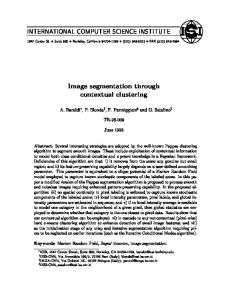
Fig. 1. MPAC algorithm for contextual image labeling. At each hierarchical level of a Laplacian Pyramid (LP) decomposition, MPAC alternates between image labeling, global, and local statistics estimation.

(3)

Fig. 2. Local estimate is not considered reliable by (3) when the number of pixels of type within window is less than the adaptive window width . Exploitation of (5) is (often) sufficient to prevent MPAC from removing isolated but genuine regions whose area is smaller . than exists and is considered • When local intensity reliable by (3), both local and global intensity estimates and , respectively) are employed for ( comparison with the pixel data according to (4). It is worth mentioning, that while testing MPAC, we found images to which the proposed version of (4) applies

where (4) and (5), shown at the bottom of the page, give the necessary conditions. Equations (3)–(5) indicate the following. • MPAC alternates between pixel labeling and global (image-wide) and local intensity parameter estimation as shown in Fig. 1. , • According to (5), when a local intensity average centered on pixel estimated in neighborhood , does not exist or is considered unreliable, then the estiis employed, mate of the global intensity average instead, for comparison with the pixel data as shown in

if if

exists and is considered reliable does not exist or is considered unreliable

(4) (5)

1836

IEEE TRANSACTIONS ON GEOSCIENCE AND REMOTE SENSING, VOL. 40, NO. 8, AUGUST 2002

truth training areas to account for within-class intensity variance). According to [11], theoretical weaknesses and limitations of the MPAC algorithm are as follows.

Fig. 2. The PAC and MPAC intensity average adaptive learning mechanism.

successfully, while a simpler version of (4) exploiting , exclusively, does not. local estimates Simultaneous exploitation of local and global class-conditional spectral statistics in (4) and (5) indicates that MPAC employs, at each resolution level of the LP decomposition, a multiresolution and adaptive criterion for spectral parameter estimation. To point out the difference between MPAC and PAC, consider that the original PAC algorithm replaces (4) and (5) with , if local average exists and is considered reliable; otherwise, label cannot be considered eligible for the th pixel labeling. This implies that PAC removes every genuine but small (isolated) region whose size is below . window width According to [11], advantages of MPAC with respect to other labeling algorithms found in the literature are as follows. 1) When compared with noncontextual clustering algorithms like the well-known Hard -Means (HCM) clustering technique [35] (which is a hard-competitive, Bayesian, noncontextual, maximum likelihood labeling procedure), MPAC is less sensitive to changes in the user-defined number of input clusters, as it allows the same region (label) type to feature different intensity averages in different parts of the image, as long as they are separated in space (in line with PAC [10]). 2) Although it employs no MRF model that supports special image features (e.g., thin lines; see [28]), MPAC preserves genuine but small regions significantly better than HCM, stochastic expectation maximization (SEM, which is a soft-competitive, Bayesian, contextual labeling procedure [30]), and PAC [10]. 3) Owing to its spectral parameter adaptation strategy and consequent robustness to changes in initial conditions, MPAC is easy to use, i.e., it requires minor user supervision. For example, parameter (related to the additive Gaussian noise standard deviation ) may be estimated from supervised training data. Moreover, to initialize MPAC successfully, isolated ground truth pixels may be sufficient (whereas traditional classifiers require ground

1) MPAC applies only to slowly varying or piecewise-constant intensity images, i.e., to images with little useful texture information and additive Gaussian noise independent of the scene. 2) It is unable to detect outliers, which may affect the estimate of spectral parameters. 3) Although it is less sensitive to changes in the user-defined number of input clusters than traditional (noncontextual) clustering algorithms, MPAC is still a suboptimal labeling procedure that is sensitive to initial conditions. Therefore, one main issue in the user interaction with MPAC remains the choice of the number of clusters to be detected. In [11], MPAC is applied to a variety of test images, including a multispectral SPOT satellite image. Based on the analysis of (1) and (2), the RS field of application of MPAC can be reasonably assessed as follows. • Due to (1), MPAC applies exclusively to images featuring little useful texture information. Since within-class spatial correlation (interpixel feature correlation, texture [4]) has been found to decrease exponentially with the dimensionality of optical images [12], [13], (1) becomes increasingly acceptable as the data dimensionality increases in remotely sensed optical imagery applications. • Due to (2), MPAC applies to piecewise-constant or slowly varying intensity images affected by a white Gaussian noise field independent of the scene. As a consequence, MPAC is not suitable for dealing with synthetic aperture radar (SAR) images affected by multiplicative speckle noise. In synthesis, based on (1) and (2), MPAC seems applicable to (unsupervised) clustering, (supervised) classification, segmentation, and quantization of remotely sensed optical images featuring little useful texture information. This potential range of RS applications is the same as that of the well-known HCM clustering algorithm, which justifies the dissemination of MPAC among the RS readership. To further investigate the trade-off between labeling performance and ease of use of MPAC against common classifiers such as the minimum-distance-to-means and the Gaussian maximum likelihood, a real and standard RS image is selected for comparison [36]. For consistency with the satellite data employed in the application example proposed further in this paper, the Landsat TM image (1024 750 pixels in size) included in the grss dfc 002 data set provided by the Geoscience and Remote Sensing Society (GRSS) Data Fusion Committee (http://www.dfc-grss.org) is chosen for classification comparison. In this test image, eight thin, elongated, and spectrally homogeneous regions of interest (ROIs) are selected by a photointerpreter. Next, an HCM clustering algorithm is run on , the entire image, with an arbitrary number of clusters which is considered sufficient to obtain a satisfactory image

SGRENZAROLI et al.: CONTEXTUAL CLUSTERING FOR IMAGE LABELING

1837

TABLE I MPAC CLASSIFIER. CONFUSION MATRIX AND ENERGY VALUES IN THE LABELING TASK OF THE GRSS DFC 002 LANDSAT TM IMAGE. THE SIZE of ROIS IS REPORTED, IN PIXEL UNITS, ON THE RIGHT COLUMN

TABLE II MINIMUM-DISTANCE-TO-MEANS CLASSIFIER. CONFUSION MATRIX AND ENERGY VALUES IN THE LABELING TASK OF LANDSAT TM IMAGE. THE SIZE OF ROIS IS REPORTED, IN PIXEL UNITS, ON THE RIGHT COLUMN

THE GRSS DFC

TABLE III GAUSSIAN MAXIMUM LIKELIHOOD CLASSIFIER. CONFUSION MATRIX AND ENERGY VALUES IN THE LABELING TASK OF LANDSAT TM IMAGE. THE SIZE OF ROIS IS REPORTED, IN PIXEL UNITS, ON THE RIGHT COLUMN

partition. These data clusters are employed to initialize the free parameters of a minimum-distance-to-means, a Gaussian maximum likelihood, and an MPAC classifier. Classification accuracies are presented in (unconventional) nonsquare confusion matrices in Tables I–III. To assess accuracy in nonsquare confusion matrices, parameter Energy (Ene) is computed as , where is the probability of a pixel belonging to the th class and th ROI, such that Ene increases when a ROI belongs to just one class. Among the three classifiers considered, MPAC features the largest value of Ene. In line with [11], this experiment points out that, when compared to two well-known noncontextual classifiers, MPAC 1) reduces salt-and-pepper classification noise; 2) recovers fine image details; 3) requires a degree of user supervision equivalent to that of HCM.

002

THE GRSS DFC

002

IV. REMOTE SENSING APPLICATION PROJECT: DEGRADED FOREST ASSESSMENT IN BRAZILIAN AMAZON A. Problem Description and Objectives The estimation of sources and sinks of greenhouse gasses resulting “from direct human-induced land use change and forestry activities, limited to afforestation, reforestation, and deforestation since 1990” is an information requirement of the Kyoto protocol compiled during the Third Conference of the Parties in the framework of the United Nations Convention on Climate Change [37]. In this scenario, which has relevant political, economic, and scientific implications, earth observations from satellites provide a valuable source of qualitative and quantitative information to investigate changes in tropical forest ecosystems caused by anthropic activities. In monitoring forestry activities from space, the Landsat Thematic Mapper (TM) is one of the most widely employed sources of remotely sensed data [38]–[42].

1838

IEEE TRANSACTIONS ON GEOSCIENCE AND REMOTE SENSING, VOL. 40, NO. 8, AUGUST 2002

In terms of information representation, a crisp and binary (vegetation/bare soil) classification approach is widely adopted to investigate deforestation phenomena. For example, several recent studies focused on areas where forest is converted into agricultural fields (clear-cut areas) in the Amazon basin [39]–[41]. Such a crisp and binary information representation is unable to describe a great variety of forest alterations that reduce the tree cover but do not eliminate it, such as those due to surface fires or selective logging in standing forest. In [14], forest areas affected by selective logging are detected on TM images of the Brazilian Amazon by means of human interpretation and digitization. Partially regrowth deforested areas are detected on TM images using a shade fraction image segmentation system in [41]. Nepstad et al. speculate that intermediate forest alterations are actually ignored by official deforestation mapping programs [15]. In this paper, the term “forest degradation” is based on a functional definition. It identifies any intermediate forest alteration that decreases the forest biomass or biodiversity. In land cover terms, the degraded forest class identifies any forest condition intermediate between those of classes forest and deforestation. This definition is in line with that adopted by the FAO according to which “(forest) degradation is not reflected in the estimates of deforestation” [43]. To summarize, although it is ignored by the Kyoto Protocol and several deforestation mapping programs, the degraded forest class may have a significant impact on the estimation of forest areas impoverished each year by anthropogenic activities [15]. To assess whether deforestation mapping programs underestimate the forest that is actually impoverished (i.e., degraded) each year, as recently speculated in [15], our application project aims at detecting forest degradation phenomena in the Brazilian Amazon from remotely sensed data. B. Study Areas Two study areas are located, respectively, in the Brazilian states of Pará and Mato Grosso, which belong to the belt of major anthropogenic pressure within the Amazon basin. In the Pará test site, the predominant vegetation is evergreen terre firme forest with above-ground biomass of 250–300 t/ha (tons/hectars). Timber extraction has become a major industry over the last 15 years, centered on Paragominas, leading to landscape of logged and “superlogged” forests, along with pasture [44]. The cycle of exploitation begins with selective logging for the most valuable species. These regions are later revisited for less lucrative timber and becomes a fragmented open canopy (superlogged forest) increasingly prone to fire [45]. In the final phase, the residual forest is cleared for pasture. The Mato Grosso test site is characterized by the presence of semi-evergreen forest and landscape transitions between cerrado and forest vegetation. Ranching and selective logging determine the deforestation pattern [46]. C. Feasibility Study To make a decision as to whether or not quantitative remote sensing is a reasonable approach to use [47], two contiguous Landsat TM scenes acquired in 1999 during the same satellite pass (path-row 222-62 and 222-63, 7781 7243 pixels in size, identified by code 2 and 3 in Fig. 3) on the Pará test site and two

Fig. 3. Three Landsat TM scenes cover the Pará and Mato Grosso test sites in the Amazon basin. Three TM subimages (identified as test1, test2, and test3) are extracted from the Pará test site along the flight path of the aerial photo campaign depicted as a black line.

multitemporal but coincident Landsat TM scenes (path-row 226-69, 7639 7307 pixels in size, identified by code 1 in Fig. 3) of the Mato Grosso test site, acquired in 1992 and 1996, respectively, are selected. The same two TM scenes of Mato Grosso were employed, respectively, by TRFIC and FAO, to develop deforestation maps. With regard to the selected TM scenes of the Pará test site, three TM subimages, 450 450 pixels in size (identified as test1, test2, and test3 in Fig. 3), are extracted to overlap with some aerial images acquired along the depicted flight path by the Brazilian Space Research Agency Instituto National de Pesquisas Espaciais (INPE) in 1999, as shown in the upper right corner of Fig. 3. In the selected four Landsat TM scenes of the Brazilian Amazon (see Fig. 3), expert photointerpreters were asked to distinguish the cover types of interest based on spectral and spatial characteristics. As a result, two forest degradation cover types are identified. The first distinguishable forest degradation phenomenon, termed class Vegetation-Bare soil (VB), consists of full-canopy forest with clearings due to selective logging. In Landsat TM images, VB areas are visually perceived as small (1–3 pixels wide), isolated, or regularly distributed bare-soil regions surrounded by forest, as shown in Fig. 4. The second type of distinguishable forest disturbance is 100% vegetate cover of pioneer species with a canopy high from 2 to 10 m, known as “capoeira.” It is visually detected as clear-cut regions, which are abandoned and/or partially regrown. These are wide areas with a regular shape whose spectral behavior is quite similar to the forest spectral signature (see Figs. 5 and 6). This second type of forest degradation phenomena is identified as class Vegetation-Forest (VF) to indicate its spectral similarity . to class Forest To provide a complete partition of the selected TM scenes, the following land cover classes are considered: 1) Water (W); 2) closed-canopy Forest (F); 3) Bare soil Agricultural areas (BA);

SGRENZAROLI et al.: CONTEXTUAL CLUSTERING FOR IMAGE LABELING

1839

Fig. 5. The second type of forest disturbance is visible in the Landsat TM 222 62 99 image (R: band5, G: band3, B : band3). White contours indicate two large regions of forest degradation featuring a regular shape and a spectral signature quite similar to that of the forest class. This second forest degradation phenomenon is identified as class Vegetation-Forest. Fig. 4. White arrows indicate the first type of forest disturbance. Isolated bare-soil targets surrounded by the forest area are visually distinguishable in the Landsat TM 226 69 92 image (R: band5, G: band4, B : band3). This forest degradation phenomenon is identified as class Vegetation-Bare Soil.

4) Degraded Forest (DF) Vegetation-Bare soil (VB) Vegetation-Forest (VF). 1) Reference Data for the Mato Grosso Test Site: The TRFIC and FAO Maps: Two deforestation maps of the Mato Grosso test site are available from TRFIC and FAO. TRFIC, which is a project of NASA’s Earth Science Information Partnership program, delivers a deforestation map, extracted from the 1992 Landsat TM scene (path-row 226-69), with a pixel size equal to 30 m and a geographic localization error of 500 m [39]. The classification method employed by TRFIC is based on image thresholding and iterative self-organizing methods. Accuracy is validated by means of field observations. Land cover types in the TRFIC map are 1) forest; 2) deforested; 3) regrowing forest; 4) water; 5) cloud; 6) cloud shadow; 7) cerrado. The FAO map, extracted from the 1996 Landsat TM scene (path-row 226-69), consists of ten cover classes detected by visual interpretation conducted at a scale of 1:200 000 [39]. Next, data were digitized and geometrically corrected using reference topographic maps. The minimum mapping unit (spatial resolution) is 100 ha. FAO classes are 1) closed-canopy forest; 2) open-canopy forest;

Fig. 6. Spectral signatures of classes Forest (F ) and Vegetation Forest are quite similar.

3) short/long fallow (forest affected by shifting cultivation); 4) mosaic forest shrubs; 5) shrubs; 6) other land cover; 7) water; 8) plantations (forest and agricultural). 2) Reference Data for the Pará Test Site: Aerial Photos: The Parà area was one of the targets of an aerial photo campaign conducted during 1999 by INPE. Images were collected using digital video along a set of flight transects across the Brazilian Amazon basin. The video data were geolocated using an on-board global positioning system, but no geometric correction was provided to recover from systematic and accidental distortions of the acquisition process. In other words, these aerial images (480 630 pixels in size with a spatial resolution of approximately 1.2 m) feature no photogrammetric quality, i.e., although they can be geolocated, their coregistration with

1840

IEEE TRANSACTIONS ON GEOSCIENCE AND REMOTE SENSING, VOL. 40, NO. 8, AUGUST 2002

Fig. 7. Comparison of class distributions in scatterograms (R; G) and (R; B ) with those in scatterograms (H; I ) and (H; S ) confirms that IHS color transformation enhances spectral separability of classes VF and VB from class Forest (F ).

satellite data is extremely difficult (requiring many target points). Small, cleared patches surrounded by forest, corresponding to degraded forest type VB, are clearly visible in aerial photos. The indicative aerial flight path over TM subimages test1 to test3 is depicted in Fig. 3. Along this aerial flight path, aerial images showing forest degradation phenomena without being affected by cloud cover are selected. The number of selected aerial images that overlap with TM subimages test1 to test3 is, respectively, 6, 4, and 6. This means that, in the Pará test site, the ground (reference) data are rather limited. As a consequence, the quantitative accuracy assessment of the TM data classification map of Pará is rather weak (i.e., vague and subjective). In this context, exploitation of the Parà test site in combination with the Mato Grosso test site becomes strategic in order to 1) collect a wide set of evidence that provides, as a whole, a reasonable (although weak) assessment of the proposed classification scheme with respect to changes in raw data properties (nonoverlapping versus overlapping and unitemporal versus multitemporal raw data) and prior knowledge representations (aerial images versus classification maps) and 2) maintain consistency with the work in [15]. D. Implementation of the Classification System To detect classes VB and VF in Landsat TM images of the Brazilian Amazon, a three-stage classification method is adopted. The first stage is a preprocessing module consisting

of an intensity-hue-saturation (IHS) color transformation capable of emphasizing quantitative (spectral) and qualitative (visual) separability of the VB and VF forest degradation phenomena. The second stage consists of the detail-preserving contextual clustering MPAC algorithm. The third stage is the output module providing a many-to-one relationship between second-stage output categories (clusters) and desired output classes (“multiple-prototype classifier” [23]). 1) Preprocessing Stage: RGB to IHS Color Transformation: While the use of all TM spectral bands may at first seem to offer a higher potential of class discrimination, our test is limited to TM bands 5 (1.55–1.75 m), 4 (0.76–0.90 m), and 3 (0.63–0.69 m) selected as channels red-green-blue (RGB), respectively. Bands 1 and 2 are frequently contaminated with smoke and haze in Amazonia, while Band 6 is at a different spatial resolution (120 m). The exclusion of Band 7 can be argued for; however, much of its information content is found in Band 5 when forest is depicted [38]. Furthermore, by using these three bands, the information content is the same employed by the major Amazon monitoring program [38], allowing for comparison with operational technique. The RGB-to-IHS color space transformation (e.g., refer to [48]) is effective in enhancing the spectral separability of supervised data belonging to classes VF and VB from class . This and to be compared is shown in scatterograms with and (see Fig. 7). Pairwise spectral divergence (Div) values, computed under the hypothesis of class-con-

SGRENZAROLI et al.: CONTEXTUAL CLUSTERING FOR IMAGE LABELING

1841

TABLE IV PAIRWISE CLASS DIVERGENCE RESULTS CONFIRM THAT THE RBG--TO-HIS COLOR TRANSFORMATION ENHANCES THE SPECTRAL SEPARABILITY OF CLASSES VF AND VB FROM CLASS F

TABLE V FISHER’S SEPARABILITY VALUES OF CLASS PAIR (F; VF) IN BANDS I , R, G, AND B

ditional normal distribution [49] and normalized with respect to the maximum spectral divergence found between class pair , are reported in Table IV. In line with the qualitative interpretation of Fig. 7, these results confirm that the RGB-to-IHS color transformation enhances the spectral separability of class by a large degree, while class pair seems pair to improve slightly. To further investigate effects of the IHS , color transform on spectral separability of class pair this pairwise spectral separability is quantitatively assessed by the Fisher linear discriminant (6) where index identifies the spectral band, while symbols and identify sample mean and standard deviation of a classconditional distribution [5]. These separability values, shown in Table V, confirm that the IHS color transformation is also capable of enhancing the spectral separability between class pair . 2) MPAC: Details on Input Parameters and Output Products: User interaction with the MPAC algorithm is restricted to selecting smoothing parameter and initial template vectors. Parameter , proportional to additive white Gaussian noise variance , is either user-defined (to be set with a trial-and-error procedure) or estimated from supervised training data. When no supervised ground truth data are available, initial template vectors may be detected by an (unsupervised) clustering algorithm (see Fig. 1). In this work, no clustering algorithm is used for MPAC initialization. Rather, some supervised (labeled) pixels are sequentially selected by an expert photointerpreter as initial template vectors (also called codewords). Of course, one or more codewords may belong to the same output class. Note that, in terms of ease of use, this type of user supervision is more convenient than selecting ground truth areas, as required by common classification approaches (both parametric and nonparametric), i.e., prior knowledge required by this system to run may be inferior to that required by traditional classifiers. Interactive training pixel selection is made easier by the IHS color transformation, which increases the spectral difference between classes , VB, and VF. To assist the user in selecting significant initial templates, MPAC generates a normalized confidence

level output map where each pixel is replaced with its relative membership value, i.e., with a normalized degree of similarity between the pixel data vector and its closest template vector. Pixels featuring low membership values are outliers, i.e., they are not represented with high confidence by the current codebook. To check whether significant image details are maintained through the MPAC processing, a piecewise-constant intensity output image is generated by substituting all pixels belonging to a segment (defined as a connected area featuring the same class type in the labeled image) with their segment-based average spectral value. A contour image depicting segment boundaries is generated too. For the Pará test site (see Fig. 3), 11 codewords (supervised pixels), each one associated with one out of five labels (see Section IV-C), are sequentially selected in the TM test1 subimage by a photointerpreter (see Fig. 3). After the MPAC learning phase, final codewords are applied to TM subimages test2 and test3 to verify the algorithm generalization capability. Other 11 supervised pixels are considered sufficient to initiate an MPAC detail-preserving clusterization of the TM scene of Mato Grosso. In these two applications, MPAC is run for 15 iterations within a two-step hierarchical procedure: first, parameter is set to 0 (i.e., MPAC follows the data); next, is set to a value for pixels belonging to classes , VF, and VB, to reduce salt-and-pepper classification noise (e.g., due to the presence of smoke and thin clouds during TM data acquisition), while the remaining classes are masked out from further refinements. For the Pará and Mato Grosso data sets, a smoothing parameter is set equal to 0.01 and 0.04, respectively, by a trial-and-error procedure. 3) Output Classification Stage: Output maps are obtained as a supervised and crisp many-to-one combination of the , , BA, 11 MPAC output categories with output classes VF, and VB. Let us show an example of the three-stage classification process. Fig. 8(a)–(f) show, respectively: test1 raw input data, 450 450 pixels in size; IHS color transformation (in false colors); (in pseudocolors); MPAC-labeled image with (in MPAC piecewise-constant intensity image with false colors); (in pseudocolors); e) MPAC-labeled image with (in f) MPAC piecewise-constant intensity image when false colors). a) b) c) d)

Fig. 8(c) and (e) are partitioned into 19 000 and 6700 segments, respectively. Comparisons of Fig. 8(b), (d), and (f) allow a visual and intuitive inspection of the classification quality. In Fig. 9 two corresponding profiles (transects) extracted from Fig. 8(b) and (d) are depicted. In line with theoretical expectations, Fig. 9 shows that, in this application, MPAC provides an information quantization (compression) equivalent to an edge-preserving smoothing capable of preserving structures 1–3 pixels wide. Image-wide histograms of Fig. 8(b) and (d) are shown in Fig. 10: whereas Fig. 8(d) looks as an accurate edge-preserving smoothed version of Fig. 8(b), the histograms of these two images look different indeed.

1842

IEEE TRANSACTIONS ON GEOSCIENCE AND REMOTE SENSING, VOL. 40, NO. 8, AUGUST 2002

Fig. 8. Three-stage classification. Input and output products on the Pará test site (subimage test1). (a) Input: Landsat TM subimage: R (Band 5), G (Band 4), B (Band 3). (b) Output of the HIS color transformation (in false colors). (c) MPAC-labeled image with 0 (in pseudocolors). (d) MPAC piecewise-constant intensity image with = 0 (in false colors). (e) MPAC-labeled image with > 0 (in pseudocolors). (f) MPAC piecewise-constant intensity image with > 0 (in false colors).

=

Fig. 9. Profiles extracted from Fig. 8(b) (thin line) and (d) (thick line).

V. EXPERIMENTAL RESULTS A. Pará Test Site: Qualitative and Quantitative Result Assessment The result validation procedure focused on the analysis of those parts of the three TM submaps (corresponding to raw subimages test1 to test3; see Fig. 3) that overlap with aerial photos and are characterized by different distributions of the VB forest degradation type as shown in Fig. 11(a)–(c). According to an expert photointerpreter, the degree of match between visually detected VB phenomena in aerial photos and automatically detected VB pixels in TM images is satisfactory [see Fig. 11(a)–(c)]. The same subjective conclusion is reached when VF degradation phenomena are examined (see Fig. 12). Since the training phase of the three-stage classifier has involved data selected from one TM subimage exclusively, these qualitative re-

Fig. 10.

Histograms of Fig. 8(b) (top) and (d) (bottom).

sults seem to indicate that the proposed classifier is also capable of generalizing. As to the quantitative assessment of classification, due to difficulties in coregistration of aerial photos with TM images, we are unable to generate a confusion matrix (see Section IV-C). As an alternative, a degraded forest fragmentation measure, such as the Perimeter-over-Area ratio (PA) [50], is adopted. In a labeled image, segments (or patches) are defined as connected image

SGRENZAROLI et al.: CONTEXTUAL CLUSTERING FOR IMAGE LABELING

1843

(a)

(b)

(c) Fig. 11. (a) Comparison between aerial photos and a TM thematic submap (see the white outline at the bottom right) in which the density of the VB degradation class is considered “high.” (b) Comparison between aerial photos and a TM thematic submap (see the white outline at the bottom right) in which the density of the VB degradation class is considered “medium.” N.B.: To make visual interpretation easier, these pictures are rotated 180 with respect to those depicted in Fig. 11(a) and (c). (c) Comparison between aerial photos and a TM thematic submap (see the white outline at the bottom right) where the density of the VB degradation class is considered “low.”

areas featuring the same label type. Intuitively, a labeled type (e.g., class forest) in a labeled image is 1) compact where it features low PA values and 2) fragmented (“patchier”) where PA values tend to increase (see Fig. 13). It is easy to prove that

PA is sensitive to the shape and size of segments (for the analysis of the distribution of patches by size, shape, or distance between patches refer to [51]). To provide (vegetation/bare soil) binary maps of aerial images, a histogram thresholding tech-

1844

IEEE TRANSACTIONS ON GEOSCIENCE AND REMOTE SENSING, VOL. 40, NO. 8, AUGUST 2002

note that class

is not considered in this analysis), in window . Probability is defined as the number divided of pixels belonging to class detected in window by the total (image-wide) number of pixels belonging to class . Probability values , are used to generate the th class-conditional histogram , where the bin size of the probability-axis is set to 0.001. Entropy of class is computed as (7)

Fig. 12. Comparison between aerial photos and a TM thematic submap where Vegetation-Forest degradation phenomena are detected.

Fig. 13.

(since is maximum when all where histogram values are equal, i.e., in case of uniform distribution, ). Table VI reports then entropy values for classes , VF, VB, and BA in each of the three TM submaps of the Pará test site. In line with theoretical expectations, classes VB and VF feature higher entropy values . when compared with classes and A third piece of evidence for the consistency of detected degraded forest type VB expected to be involved with high-change forest dynamics is shown in Fig. 14, where TM image areas with label VB (likely to be related to selective logging) become new clear cuts in aerial photos acquired about two months later. In terms of overall statistics, the three TM thematic submaps, 450 450 pixels in size, cover a surface area of approximately 18 225 ha each. In these submaps, class VF varies from a minimum of approximately 1224 ha (6.8% of the ground coverage) to a maximum of 4730 ha (25.9%), and class VB ranges from approximately 1297 ha (7.0%) to a maximum of 5143 ha (28.0%). In the three TM thematic submaps, class DF covers a minimum of 13% up to a maximum of 45% of the image ground coverage. This result is in line with the work in [14], which estimated a forest alteration of 12% due to selective logging (related to class VB) in the Brazilian State of Pará from the years 1988–1991.

Examples of PA value extraction.

B. Mato Grosso Test Site: Result Assessment nique is adopted. Next, PAs are computed for 1) the (vegetation/bare soil) binary aerial maps, where PA equals 3.7, 2.8, and 2.0, respectively, and 2) the VB class detected in the three TM submaps, where PA equals 0.7, 0.4, and 0.2, respectively (class VF, characterized by large homogeneous areas with a regular shape, has no significant fragmentation). The correlation coefficient between the two PA sequences is 0.99. Unfortunately, this evidence is weak because only three data points per sequence are used, due to the limited availability of meaningful aerial photos. Thus, to further assess the consistency of the degraded forest information provided by the three TM submaps of the Parà test site, the spatial distribution of classes VB and VF is examined. This distribution is relevant because the homogeneity in distribution of VB patches within forest areas is expected to increase with the anthropogenic pressure on forest ecosystems. To estimate the spatial distribution of classes, a spatial entropy measure (Ent) is adopted as follows. First, each TM thematic submap (450 450 pixels in size) is partitioned into 30 nonoverlapping , 15 15 pixels in size. Second, windows is computed for class probability (corresponding to classes , VF, VB, and BA, respectively;

In the Mato Grosso test site, the two selected multitemporal TM scenes, 1245 1245 pixels in size, cover an area of approximately 139 502 ha (for geographical location see Fig. 3). In the two TM data maps, the VF class extension is approximately 9141 ha (6.5%) in 1992 and 13 175 ha (9.4%) in 1996. Extension of class VB is approximately 17 612 ha (12.6%) in 1992 and 8922 ha (6.4%) in 1996. To compare the 1992 TM data map with the TRFIC deforestation map, first, the TRFIC classes are reduced to label types water, forest, and nonforest, where metaclass nonforest is the combination of TRFICs classes deforested, regrowing forest, and cerrado (the TRFIC classes cloud and cloud shadow are absent from the area of interest). Second, cover types of the TM classification map are reduced to classes water, forest, and nonforest, by aggregating classes VF, VB, and BA into the nonforest metaclass. Finally, from these two reaggregated maps, classification statistics of classes water, forest, and nonforest are computed as shown in Table VII. This table points out that, overall, the three-stage classifier assigns to the forest class 13.0% fewer pixels than the TRFIC map. Conversely, the three-stage classification system assigns to the

SGRENZAROLI et al.: CONTEXTUAL CLUSTERING FOR IMAGE LABELING

1845

TABLE VI ENTROPY VALUES

F

W

FOR THE SPATIAL DISTRIBUTION OF CLASSES , VF, VB, AND BA (CLASS IN EACH OF THE THREE TM THEMATIC SUBMAPS OF THE PARÀ TEST SITE

Fig. 14. High-change dynamics of areas affected by forest degradation phenomena. Class Vegetation-Bare soil (VB) detected in the Landsat TM image becomes new clear cuts in aerial photos taken about two months later, where recently cut trunks are still on the ground (localize the river to link the aerial photo sequence with the TM image and corresponding thematic map). TABLE VII COMPARISON BETWEEN THE TRFIC CLASSIFICATION AND THE MPAC-BASED THREE-STAGE CLASSIFIER. CLASSES WATER, FOREST, AND NONFOREST ARE CONSIDERED FOR COMPARISON

nonforest metaclass 12.8% more pixels than the TRFIC map. To understand the cause of such discrepancies, a confusion matrix is reported in Table VIII, where the percentage of nonforest pixels detected by the three-stage classifier is presented according to its class components BA, VB, and VF. This table % % of the shows that, respectively, 18.2% % % of the TRFIC forest metaclass and 21.6% TRFIC nonforest metaclass overlap with TM forest degradation areas. These percentages are equivalent to a ground coverage ha ha), corresponding to 19.1% of 26 723 ha ( ha ha) of the total surface coverage. ( Note that 55% of the TRFIC water class (equivalent to 30 ha) overlaps with forest degradation types VB and VF.

IS

NOT

CONSIDERED)

With regard to the 1996 FAO classifications map of the Mato Grosso test site, a direct comparison with the 1996 TM data map is difficult because 1) the FAO land-use/land-cover legend is quite different from land cover classes detected by the threestage classifier and 2) the two output maps employ different minimum mapping units, equal to 100 ha (resampled to a pixel size equal to 100 m) for the FAO map and one pixel size equal to 30 m for the TM thematic map, respectively. To provide a comparison, the following strategy is adopted. First, the TM classification map is subsampled at pixel size of 100 m. Next, the subsampled TM data map, the FAO map, and the corresponding Landsat TM 226-69 (1996) image are visually compared by an expert photointerpreter, as shown in Fig. 15. This qualitative inspection confirms that the FAO closed-canopy forest class overlaps with forest degradation phenomena detected in TM data (no FAO open-canopy forest is present in this area of interest). Quantitatively, the FAO closed-canopy forest class exceeds by approximately 10% the class forest detected by the three-stage classifier. In particular, class VF appears to be the first cause of discrepancies between the two maps. Sometimes, the VF class overlaps with the FAO mosaic forest shrubs class, although it is generally included in the FAO closed-canopy forest class. With regard to the VB forest degradation class, it overlaps with the FAO classes short/long fallow, closed-canopy forest, other land covers, and shrubs in decreasing order. VI. SUMMARY AND CONCLUSIONS The MPAC algorithm, recently published in the image processing literature, is proposed as a valuable tool in clustering, classification, segmentation, and quantization of remotely sensed images where texture information is negligible. Owing to its contextual, adaptive, and multiresolution labeling approach, MPAC is capable of preserving genuine but small regions, is easy to use (e.g., supervised selection of one pixel per spectral category suffices to obtain image partitions where image details are likely to be preserved), and is robust to changes in input parameters. By requiring minor supervision, MPAC seems particularly useful for monitoring areas where ground truth data are difficult to collect. Proper selection of a smoothing parameter may help reducing salt-and-pepper classification effects. As a remote sensing application example, an MPAC-based three-stage classifier is applied to degraded forest detection in Landsat TM scenes of the Brazilian Amazon, where intermediate states of forest alterations caused by anthropogenic activities can be characterized by image structures one to three pixels wide. Two tropical forest degradation phenomena (VF and VB) and five classes of interest ( , VF, VB, BA, and

1846

IEEE TRANSACTIONS ON GEOSCIENCE AND REMOTE SENSING, VOL. 40, NO. 8, AUGUST 2002

TABLE VIII CONFUSION MATRIX BETWEEN THE TRFIC CLASSIFICATION AND THE MPAC-BASED THREE-STAGE CLASSIFIER. PIXELS BELONGING TO THE NONFOREST METACLASS DETECTED BY THE MPAC-BASED CLASSIFIER ARE DIVIDED INTO ELEMENTARY CLASSES BA, VB, AND VF

Fig. 15.

Comparison between a Landsat TM 226-69 (1996) subimage, the corresponding TM thematic submap (subsampled at 100 m), and the FAO submap.

) are identified by expert photointerpreters. In the Pará test site, VF and VB patches detected by the three-stage classifier are validated as anthropic disturbances against the background of forest cover by qualitative and (rather weak but numerous) quantitative comparisons with aerial photos. This investigation shows that, in three 1999 TM data submaps, forest degradation phenomena account for 13% up to 45%. This result is in line with [14], which estimated a forest alteration of 12% due to selective logging in the Brazilian state of Pará from the years 1988–1991. In the Mato Grosso test site, two maps generated from a 1992 and a 1996 TM data scene reveal that forest degradation areas 1) account for, respectively, 19% and 16% of the ground coverage and 2) overlap with 10% and 18% of the forest class detected by the FAO and TRFIC deforestation mapping programs in

1992 and 1996, respectively. This result is in line with the work in [15], which speculates that present estimates of annual deforestation for the Brazilian Amazon capture less than half of the forest area that is impoverished each year. In synthesis, the novelty of the degraded forest classification method is relevant if we consider the following. i) The proposed classification scheme guarantees a good compromise between accuracy and ease of use, whereas detection of (crisp, binary) deforestation phenomena at regional scales and high spatial resolutions still depends, to a large extent, on human photointerpretation. ii) Although intermediate forest alterations have a significant impact on the assessment of forest areas impoverished each year by anthropogenic activities, no degraded forest estimation is required by the Kyoto

SGRENZAROLI et al.: CONTEXTUAL CLUSTERING FOR IMAGE LABELING

Protocol and provided by official deforestation mapping programs (such as those by FAO and TRFIC). ACKNOWLEDGMENT The authors wish to thank the Brazilian Space Agency (INPE), for allowing them to take part in the 1999 aerial campaign. Special thanks go to A. Setzer, the campaign organizer, and the pilots of the airplane Bandeirante. They are also grateful to the anonymous referees for their thoughtful comments about this paper. P. C. Smits, as a member of the GRSS-DFC, is acknowledged for providing the grss dfc 0002 Landsat TM image. REFERENCES [1] P. Zamperoni, “Plus ça va, moins ça va,” Pattern Recognit. Lett., vol. 17, no. 7, pp. 671–677, 1996. [2] R. C. Jain and T. O. Binford, “Ignorance, myopia and naiveté in computer vision systems,” Comput. Vision, Graph., Image Process.: Image Understanding, vol. 53, pp. 112–117, 1991. [3] M. Kunt, “Comments on ‘dialogue,’ a series of articles generated by the paper entitled ‘Ignorance, myopia and naivete’ in computer vision systems’,” Comput. Vision, Graph., Image Process.: Image Understanding, vol. 54, pp. 428–429, 1991. [4] P. C. Smits and S. G. Dellepiane, “Synthetic aperture radar image segmentation by a detail preserving Markov random field approach,” IEEE Trans. Geosci. Remote Sensing, vol. 35, pp. 844–857, July 1997. [5] C. M. Bishop, Neural Networks for Pattern Recognition, Oxford, U.K.: Clarendon Press, 1995. [6] V. Cherkassky and F. Mulier, Learning from Data: Concepts, Theory, and Methods. New York: Wiley, 1998. [7] T. Mitchell, Machine Learning. New York: McGraw-Hill, 1997. [8] S. Krishnamachari and R. Chellappa, “Multiresolution Gauss-Markov random filed models for texture segmentation,” IEEE Trans. Image Processing, vol. 6, pp. 251–267, Feb. 1997. [9] M. Sgrenzaroli, G. F. De Grandi, H. Eva, and F. Achard, “Tropical forest cover monitoring: Estimates and validation from the GRFM JERS-1 radar mosaics using using wavelet zooming techniques,” Int. J. Remote Sens., vol. 23, no. 7, pp. 1329–1355, Apr.. [10] T. N. Pappas, “An adaptive clustering algorithm for image segmentation,” IEEE Trans. Signal Processing, vol. 3, pp. 162–177, Feb. 1992. [11] A. Baraldi, P. Blonda, F. Parmiggiani, and G. Satalino, “Contextual clustering for image segmentation,” Opt. Eng., vol. 39, no. 4, pp. 1–17, Apr. 2000. [12] Y. Jhung and P. H. Swain, “Bayesian contextual classification based on modified -estimates and Markov random fields,” IEEE Trans. Geosci. Remote Sensing, vol. 34, pp. 67–75, Jan. 1996. [13] C. Bouman and M. Shapiro, “A multiscale random field model for Bayesian image segmentation,” IEEE Trans. Image Processing, vol. 3, pp. 162–177, Feb. 1994. [14] A. Stone and T. P. Lefebvre, “Using multi-temporal satellite data to evaluate selective-logging in Pará, Brazil,” Int. J. Remote Sens., vol. 19, no. 13, pp. 2517–2526, 1998. [15] C. D. Nepstad, A. Verissimo, A. Alencart, C. Nobre, E. Lima, P. Lefebvre, P. Schlesinger, C. Potter, P. Moutinho, E. Mendoza, M. Cochrane, and V. Brooks, “Large-scale impoverishment of Amazonian forests by logging and fire,” Nature, vol. 398, pp. 505–508, Apr. 1999. [16] M. J. Barnsley and S. L. Barr, “Inferring urban land use from satellite sensor images using kernel-based spatial reclassification,” Photogram. Eng. Remote Sens., vol. 62, no. 8, pp. 949–958, Aug. 1996. [17] F. J. Cortijo and N. Perez de la Blanca, “Improving classical contextual classifications,” Int. J. Remote Sens., vol. 19, no. 8, pp. 1591–1613, 1998. [18] I. Kanellopoulos and G. G. Wilkinson, “Strategies and best practice for neural network image classification,” Int. J. Remote Sens., vol. 18, no. 4, pp. 711–725, 1997. [19] E. J. Kaminsky, H. Barad, and W. Brown, “Textural neural network and version space classifers for remote sensing,” Int. J. Remote Sens., vol. 18, no. 4, pp. 741–762, 1997. [20] A. K. Jain and F. Farrokhnia, “Unsupervised texture segmentation using gabor filters,” Pattern Recognit., vol. 24, no. 12, pp. 1167–1186, 1991. [21] M. Ceccarelli and A. Petrosino, “Multi-feature adaptive classifiers for SAR image segmentation,” Neurocomput., vol. 14, pp. 345–363, 1997.

M

1847

[22] N. Petkov, “Biologically motivated image classification system,” in Real-Time Imaging, P. A. Laplante and A. D. Stoyenko, Eds. New York: IEEE Press, 1996, pp. 195–223. [23] A. Baraldi, P. Blonda, G. Satalino, A. D’Addabbo, and C. Tarantino, “RBF two-stage learning networks exploiting supervised data in the selection of hidden unit parameters: An application to SAR data classification,” in Proc. IGARSS, Honolulu, HI, 2000, pp. 672–674. [24] E. Binaghi, I. Gallo, and I. Pepe, A cognitive pyramid for contextual classification of remote sensing images, in Geospatial Pattern Recognition, E. Binaghi, S. B. Serpico, and P. A. Brivio, Eds., to be published. [25] S. Geman and D. Geman, “Stochastic relaxation, Gibbs distributions, and the Bayesian restoration of images,” IEEE Trans. Pattern Anal. Machine Intell., vol. 6, pp. 721–741, June 1984. [26] J. Besag, “On the statistical analysis of dirty pictures,” J. R. Stat. Soc. B, vol. 48, no. 3, pp. 259–302, 1986. [27] E. Rignot and R. Chellappa, “Segmentation of polarimetric synthetic aperture radar data,” IEEE Trans. Image Processing, vol. 1, pp. 281–300, July 1992. [28] D. Geman and B. Jedynak, “An active testing model for tracking roads in satellite images,” IEEE Trans. Pattern Anal. Machine Intell., vol. 18, pp. 1–13, Jan. 1996. [29] J. Zhang, J. W. Modestino, and D. A. Langan, “Maximum likelihood parameter estimation for unsupervised stochastic model-based image segmentation,” IEEE Trans. Image Processing, vol. 3, pp. 404–419, July 1994. [30] J. Dehemedhki, M. F. Daemi, and P. M. Mather, “An adaptive stochastic approach for soft segmentation of remotely sensed images,” in Proc. Int. Workshop Soft Computing Remote Sensing Data Analysis (1995), E. Binaghi, P. A. Brivio, and A. Rampini, Eds., Milan, Italy, 1996, pp. 211–221. [31] C. Bouman and B. Liu, “Multiple resolution segmentation of textured images,” IEEE Trans. Pattern Anal. Machine Intell., vol. 13, pp. 99–113, Feb. 1991. [32] F. Girosi, M. Jones, and T. Poggio, “Regularization theory and neural network architectures,” Neural Comput., vol. 7, pp. 219–269, 1995. [33] P. Burt and E. Adelson, “The Laplacian pyramid as a compact image code,” IEEE Trans. Commun., vol. COM-31, no. 4, pp. 532–540, 1983. [34] I. M. Elfadel and R. W. Picard, “Gibbs random fields, cooccurrences, and texture modeling,” IEEE Trans. Pattern Anal. Machine Intell., vol. 16, pp. 24–37, Jan. 1994. [35] A. K. Jain and R. C. Dubes, Algorithms for Clustering Data. Upper Saddle River, NJ: Prentice-Hall, 1988. [36] L. Prechelt, “A quantitative study of experimental evaluations of neural network learning algorithms: Current research practice,” Neural Networks, vol. 9, no. 3, pp. 457–462, 1996. [37] UNEP/IUC, “The Kyoto Protocol to the Convention on Climate Change,” UNEP/IUC Executive Center, Geneva, Switzerland, 3rd ed., 1999. [38] INPE, “PRODES: Assessment of feforestation in Brazilian Amazonia,” Instituto National de Pesquisas Espaciais, Sao Paulo, Brazil, 1996. [39] Tropical Rain Forest Information Center Web site, Tropical Rain Forest Information Center. [Online]. Available: http://bsrsi.msu.edu/ trfic/index.html. [40] FAO, “Forest Resources Assessment 1990; Survey of Tropical Forest Cover and Study of Change Processes,” FAO, Rome, FAO Forestry Paper 130, 1996. [41] Y. E. Shimabukuro, G. T. Batista, E. M. K. Mello, J. C. Moreira, and V. Duarte, “Using shade fraction image segmentation to evaluate deforestation in Landsat Thematic Mapper images of the Amazon region,” Int. J. Remote Sens., vol. 19, no. 13, pp. 535–541, 1998. [42] D. Skole and C. J. Tucker, “Evidence for tropical deforestation, fragmented habitat, and adversely affected habitat in the Brazilian Amazon: 1978–1988,” Science, vol. 260, pp. 1905–1910, 1993. [43] FAO. Forest Resources Assessment 1990—Global Synthesis. FAO. [Online]. Available: http://www.fao.org/forestry/for/fra/fo124e/gep05.htm. [44] C. Uhl and I. C. Vieira, “Ecological impacts of selective logging in the Brazilian Amazon: A case study from the paragominas region of the state of Pará,” Biotropica, vol. 21, no. 2, pp. 98–106, 1989. [45] M. A. Cochrane, A. Alencar, M. D. Schulze Jr., C. M. Souza, D. Nepstad, P. Lefebvre, and E. A. Davidson, “Positive feedbacks in the fire dynamic of closed canopy tropical forests,” Science, vol. 284, pp. 1832–1835, 1999. [46] F. Achard, H. D. Eva, A. Glinni, P. Mayaux, H. J. Stibig, and T. Richards, Identification of Deforestation Hot Spot Areas in the Humid Tropics, ser. TREES Publ. Series B4. Luxembourg, EUR 18 079 EN, 100: European Commission, 1998. [47] J. C. Lindenlaub and S. M. Davis, “Applying the quantitative approach,” in Remote Sensing: The Quantitative Approach, P. H. Swain and S. M. Davis, Eds. New York: McGraw Hill, 1978, pp. 290–335.

1848

IEEE TRANSACTIONS ON GEOSCIENCE AND REMOTE SENSING, VOL. 40, NO. 8, AUGUST 2002

[48] M. P. Mather, Ed., Computer Processing of Remotely Sensed Images, 5th ed. New York: Wiley, 1987. [49] A. Singh, “Spectral separability of tropical forest cover classes,” Int. J. Remote Sens., vol. 8, pp. 971–979, 1987. [50] C. A. Johnston, Geographic Information Systems in Ecology, Oxford: Blackwell Science, 1998. [51] P. Peralta and P. Mather, “An analysis of deforestation patterns in the extractive reserves of acre, Amazonia from satellite imagery: A landscape ecological approach,” Int. J. Remote Sens., vol. 21, no. 13–14, pp. 2555–2570, 2000.

Hugh Eva is a Research Officer at the European Commission Joint Research Centre, Ispra, Italy. He is currently responsible for producing the South American map of the Global Land Cover 2000 mapping exercise. Before this, he was the Latin America coordinator of the TREES (Tropical Ecosystem Environment Observation by Satellite) project, which was set up to monitor and measure changes in the tropical forest belt, using remote sensing techniques.

Matteo Sgrenzaroli was born in Italy in 1972. He received the degree in environmental engineering from Politecnico of Milano, in 1997. In 1997, he was involved with the South East Asia Radar Rice Investigation (SEARRI) project of the Space Application Institute (SAI), European Commission Joint Research Centre (EC-JRC), in the analyses of multitemporal ERS-1 and JERS-1 SAR data. In 1998, he took part in the organization of and participated in the Changri Nup glacier monitoring expedition, promoted by University of Brescia, within the context of the EV-K2 project of National Council of Research of Italy (CNR) for a Himalaya glacier survey using ground-penetrating radar. In 1999, he was admitted to the Ph.D. program of the Wageningen Agricultural University, Wageningen, The Netherlands. He worked as a Ph.D. fellow at SAI (EC-EU) for the exploitation of JERS-1 Radar Mosaic for Tropical deforestation monitoring from 1999 to 2001. Since October 2001, he has been working with 3DVeritas, a company spin-off from the EC-JRC, founded in 2001, as project manager in the development of a 3-D surface modeling commercial software toolbox employing laser scanner data and digital images as input data.

Gianfranco De Grandi (M’90–SM’96–F’02) received the Ph.D. degree in physics engineering (with honors) from the Politecnico Milano, Milan, Italy, in 1973. Since 1977, he has been with the European Commission Joint Research Centre (JRC), Ispra, Italy, where he has performed research in signal processing for application areas such as gamma ray spectroscopy, data communications, and radar remote sensing. In 1985, he was visiting scientist at Bell Communications Research, Morristown, NJ, where he participated in the design of METROCORE, one of the first research projects for Gb rate metropolitan area networks. From 1986 to 1989, he headed the signal processing section of the Electronics Division, JRC, where he introduced VLSI design technology and conducted research, in cooperation with Bellcore, on packet video, and in cooperation with ITALTEL Italy on the European digital mobile phone network. In 1989, he joined the Institute for Remote Sensing Applications, where he started a research activity in radar polarimetry in the Advanced Techniques unit. Since 1994, he took the position of principal scientist for radar R/D in the Monitoring of the Tropical Vegetation unit, now part of the JRC Institute for Environment and Sustainability (IES). From 1997 to 2001, he has served as Assistant Professor with the Faculte’ de Feresterie et Geomatique, Universite’ Laval, Quebec, PQ, Canada. His current research interests span a wide gamut, including global-scale forest mapping using high-resolution spaceborne SAR, multiresolution analyses of SAR data based on the wavelet representation, backscattering multitemporal estimators, topography sensing using polarimetric SAR data, and the statistics of polarimetric synthesized SAR images. Dr. De Grandi is a member of the IEEE Geoscience and Remote Sensing society, the Signal Processing society, and the Planetary Society, Pasadena CA.

Andrea Baraldi was born in Modena, Italy, in 1963. He graduated in electronic engineering from the University of Bologna, Bologna, Italy, in 1989. His master’s thesis focused on the development of unsupervised clustering algorithms for optical satellite imagery. From 1989 to 1990, he worked as a Research Associate at CIOC-CNR, an Institute of the National Research Council (CNR), Bologna, Italy, and served in the army at the Istituto Geografico Militare, Florence, Italy, working on satellite image classifiers and GIS. As a consultant at ESA-ESRIN, Frascati, Italy, he worked on object-oriented applications for GIS from 1991 to 1993. From 1997 to 1999, he joined the International Computer Science Institute, Berkeley, CA, with a postdoctoral fellowship in Artificial Intelligence. Since his master’s thesis, he has continued his collaboration with ISAO-CNR in Bologna. As a Postdoctoral Researcher, he currently works at the European Commission Joint Research Centre, Ispra, Italy, in the development and validation of algorithms for the automatic thematic information extraction from wide-area radar maps of forest ecosystems. His main research interests center on image segmentation and classification, with special emphasis on texture analysis and neural network applications employing contextual image information.

Frédéric Achard studied at the Ecole Polytechnique, Paris, France (1981–1984), at the Ecole Nationale du Génie Rural, des Eaux et des Forêts, Paris, France (1984–1986), and received the Ph.D. degree in tropical ecology and remote sensing (with honors) from Toulouse University, Toulouse, France, in 1989. From 1986 to 1990, he has been at the Institute for the International Vegetation Map (CNRS/University), Toulouse, France, where he performed research in optical remote sensing techniques for monitoring vegetation dynamics in West Africa. In 1990 and 1991, he was Detached National Expert from the French Ministry of Agriculture and Forest working at the Joint Research Centre, Ispra, Italy, where he started a research activity over Southeast Asia in the framework Tropical Ecosystem Environment observations by Space (TREES) project. In 1992, he joined the European Commission Joint Research Centre (JRC), Ispara, Italy, to conduct the first phase of the TREES project. From 1996 to 2001, he led the second phase of the TREES project in the Global Vegetation Monitoring unit now part of the JRC Institute for Environment and Sustainability (IES) and initiated in 1999 activities of forest cover monitoring in Siberia. His current research interests include development of earth observation techniques for tropical and boreal forest regional assessments and for global tropical forest monitoring.