Control Charts for Variables with Specified Process Capability Indices

International Journal of Probability and Statistics 2012, 1(4): 101-110 DOI: 10.5923/j.ijps.20120104.03

Control Charts for Variables with Specified Process Capability Indices J. Subramani1,* , S. Balamurali2 1

Department of Statistics, Pondicherry University, R V Nagar, Kalapet, Puducherry, 605 014, India Department of Computer Applications, Kalasalingam University, Krishnankoil, 6426 190, Srivilliputhur,Tamilnadu, India

2

Abstract Control charts, also known as Shewhart charts in statistical process control are the statistical tools used to determine whether a manufacturing process is in a state of statistical control or not. If analysis of the control chart indicates that the process is currently under statistical control (i.e. is stable, with variation only co ming fro m sources common to the process) then no corrections or changes to process control parameters are needed or desirable. In addition, data fro m the controlled process can be used to predict the future performance of the process with the help of process capability indices. That is, the suitability and the performance of the manufacturing process are assessed in two stage processes namely control charts and process capability indices. Th is paper deals with the techniques namely, capability based control charts which combines the two stage processes into a single stage process in industrial applicat ions for on line process control. The relative performance of the capability based control charts for variables is assessed with that of existing usual control charts for variables, namely X − Charts and R − Charts . It is observed that the proposed method is simp le to apply and does not warrant any tedious computations both for control charts and for co mputing process capability indices. Fo r the sake o f convenience we have presented the control charts constants for constructing capability based R − Charts and X − Charts . The proposed method is also illustrated with the help of a numerical examp le. Keywords Control Charts, Industrial Applicat ions, Process Capability Index, Quality Characteristics

1. Introduction The present scenario of total quality management demands the effective use of statistical tools for analyzing quality problems and improving the performance of production process. Measuring, monitoring and maintaining several quality characteristics to achieve further improvements are required in every production process. Many of the quality characteristics are measurable in nature and can be expressed in terms of nu merical measurement by measuring them using micro meter, vernier calipers etc. For example, length, diameter, weight, pocket width, distance and groove diameter of a shaft are some of the quantifiab le quality characteristics encountered during the production of shafts. When dealing with measurable quality characteristics, it is usually necessary to monitor the behaviour of the mean value of the quality characteristics and its variab ility. To study the behaviour of the production process and to take a necessary action on the process, control charts for variables are very much used wh ich requ ires to co llect rando m samples fro m the production process and to compute the * Corresponding author: [email protected] (J. Subramani) Published online at http://journal.sapub.org/ijps Copyright © 2012 Scientific & Academic Publishing. All Rights Reserved

estimate of the quality characteristics. Further one has to show that the process is under statistical control before computing the process capability indices. Nowadays process capability analysis is a mandatory requirement and to have a minimu m prescribed value for the process capability indices

Cp

and

C pk

to be a supplier for original manufacturing

companies, particularly in the field of automobile industries. Process capability indices (PCI) have proliferated in both use and variety during the last three decades. Their widespread and often uncritical use led to imp rovements in quality. Process capability indices are considered as a practical tool by many advocates of the statistical process control industry. They are used to determine whether the manufacturing process is capable of producing units within the product or process specifications. A capability index is a dimensionless measure based on the process parameters and the process specifications, designed to quantify, in a simp le and easily understood way, the performance of the process. Several process capability indices have been developed among wh ich the basic and widely used indices are C p and Cpk. (see Kane[8]). A detailed review of the process capability indices can be seen in Kotz and Johnson[9]. The process capability indices are unit less measures showing the capability of a manufacturing process whether it is capable of operating within its specifications limits. If the value of the PCI exceeds one, then the process is considered

J. Subramani et al.: Control Charts for Variables with Specified Process Capability Indices

102

to be satisfactory or capable. However th is approach ignores the fact that these PCIs are rando m variables with distributions. Confidence limits play a major ro le for the correct interpretation of PCIs. Recently, techniques and tables were developed to construct confidence limits for the process capability indices. These techniques are based on the assumption that the underlying process is normal. Moreover, since many processes can frequently have skewed or heavily tailed distributions. In practice, the interval estimation technique that is free fro m the assumption of distribution is desirable. The various other properties and the behaviour of process capability indices at different type of distributions were studied by many authors. For example, the 95% confidence limits for the process capability indices Cp and Cpk were constructed by Chou, Owen and Bo rrego[5]. As their limits on Cpk can produce 97% or 98% lower confidence limits (instead of 95%) making them conservative, an approximation presented by Bissell[4] is reco mmended. Franklin and Wasserman[6] presented an init ial study of the properties of these three bootstrap confidence intervals for Cpk. Franklin and Wasserman[7] constructed the confidence limits for some basic capability indices and examined their behaviors when the underlying process is normal, skewed or heavily tailed distributions. Balamurali and Kalyanasundara m[3] constructed bootstrap confidence limits for the capability indices Cp , Cpk and Cpm based on lognormal and chi-squared distributions. Balamu rali[2] considered the above capability indices under short run production processes and constructed the confidence limits. However the problems one has to face are the following: There is a considerable time taken for establishing and monitoring the process through control charts for variables; inadequate technical personnel to correctly interpret the outcome of the control charts; unnecessary inventory and delay due to the computation of process capability indices and to take a decision on the process based on the resulting values of process capability indices. Hence it is felt to have an alternative method to achieve the benefit of both control charts for variables and the process capability analysis. As a result we have proposed new type of control charts for variables based on the required process capability indices C p

and

C pk

, called as “control charts for variables with

specified value for process capability indices”. Further we have presented the control charts constants to construct the proposed control charts and are explained with the help of a numerical examp le. For a more detailed discussion on the control charts for variab les and process capability analysis, the readers are referred to Montgomery[10], Spiring[11], Sarkar and Pal[1], Subraman i[12, 13], Subramani and Balamurali[14] and the references cited therein. In this paper, we propose a capability based control chart for on line process control. The relat ive performance o f this control charts for variables is assessed with that of existing usual control charts for variables. It is observed that the proposed method is simple to apply and does not warrant any tedious computations both for control charts and for computing

process capability indices. We are also presenting the control charts constants for constructing capability based control charts. The proposed method is also illustrated with a numerical examp le.

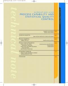
2. Control Charts and Process Capability Analysis 2.1. Usual Method Set the m anufactur ing pr ocess Im plem ent contr ol char ts for var iables Is R-Char t Under Contr ol?

No

Yes Is X-bar -Char t Under Contr ol?

No

Yes Com pute Pr ocess capability Indices Cp and Cpk Is Cp Value OK?

No

Yes Is Cpk Value OK?

No

Yes Establish the m anufactur ing pr ocess Continue the m anufactur ing Yes

Do you want to im pr ove the pr ocess?

No

Figure 1. Present M anufacturing System

For the sake of convenience to the readers, we have presented the control charts for variables for checking whether the process is under statistical control or not. That is, to take a decision whether the process can be allowed further without making any adjustment or to take corrective actions if any, to bring back the process under statistical control. Once the process has been brought under the state of statistical control by both R − Chart and X − Chart then the process capability indices

C p and C pk can be co mputed.

If the values of the process capability indices are at the satisfactory level, the process can be allowed further without making any change or adjustment in the process. Otherwise suitable adjustments have to be made so that the process shall satisfy both the requirements of control charts and the process capability indices. The present manufacturing

International Journal of Probability and Statistics 2012, 1(4): 101-110

process can be explained in the flo w chart as shown in Figure 1. The following are the various computational fo rmulae involved in constructing the control charts and for the computation of process capability indices.

1 n ∑ xi : Mean of ith samp le n i =1 1 N X = ∑ xi : Grand Mean N i =1 = Ri Max( xi ) − Min( xi ) : Range of ith samp le Xi =

R=

1 k ∑ Ri : Mean of Range values k i =1

UCLx= X + A2 R : Upper Control Limit for X -Chart LCLx= X − A2 R : Lo wer Control Limit for X -Chart

UCLR = D4 R : Upper Control Limit for R-Chart LCLR = D3 R : Lo wer Control Limit for R-Chart USL − LSL Cp = : Process Capability 6R / d2 C pu =

USL − X : Upper Process Capability Index 3R / d 2

C pl =

X − LSL : Lower Process Capability Index 3R / d 2

2.2. Proposed Method- Control Charts for Variables with Specified C p Value Suppose that a customer wants to have products produced in a process with a specified value for the process capability

index C p . To achieve this, the manufacturer has to establish a process under statistical control and then the process capability index has to be computed. If the computed value of

Cp

is more than the specified value given by the

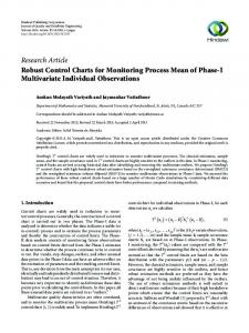
customer, the process can be run without any adjustment. Otherwise suitable actions have to be taken to meet the required process capability values. The drawback of this method is that the manufacturer has to keep all the produced items in the inventory until the co mputation of the process capability index and to take a decision on the process based on the process capability index. It is a time consuming procedure as well as requires addit ional skilled personnel. To avoid this, we have proposed control charts for variables with specified p rocess capability indices. In the proposed method, the process is under statistical control means that it satisfies the required process capability index. Further it is not necessary to compute the process capability indices separately. The proposed manufacturing process can be explained in the flow chart shown in Figure 2. Specify Cp and Cpk

Implement control charts for variables with Cp and Cpk

C pk = Min(C pu , C pl ) : Process Capability Index

Set the manufacturing process

Tolerance = T = USL − LSL USL + LSL 2 Specification Limit of

T arg et = M =

Is R-Chart Under Control?

LSL: Lower the Quality Characteristics USL: Upper Specification Limit of the Quality Characteristics When the sample size n =5, the values for the control chart constants obtained from the table are as given below: D4 = 2.114, D3 = 0, d 2 = 2.326 and A 2 = 0.577 The Control limits for constructing R − Charts and

No

Yes Establish the manufacturing process Continue the manufacturing

CLR = R UCLR = D4 R

No

Yes Is X-bar-Chart Under Control?

X − Charts are as given below: Control limits for R − Chart :

LCLR = D3 R

103

Yes

Do you want to improve the process?

No

Control limits for X − Chart :

CLx = X

Figure 2. Present M anufacturing System

LCLx= X − A2 R

The following are the derivation of various computational formulae involved in constructing the proposed control

UCLx= X + A2 R

charts with specified process capability index C p .

J. Subramani et al.: Control Charts for Variables with Specified Process Capability Indices

104

Consider C p =

USL − LSL 6σ

Where D3* =

T ⇒ Cp = 6R / d2

If

C p value is g iven then R

the above formula as R =

In the similar manner one can compute the control limits to construct X − Chart with specified

T d * ⇒R= D* Where D = 2 Cp 6

* Center Line= CLR= R= D

C p value as given

below.

Similarly one can obtain the lower control limit (LCL) and upper control limit (UCL) of the R − Chart as given below:

UCLR = D4 R

D4 d 2T ⇒ UCLR = 6C p

value can be obtained fro m

d 2T 6C p

D3d 2 6

Center line= CLX = X Lower control limit for the proposed X − Chart is obtained as given below:

LCLx= X − A2 R

T Cp

⇒ LCLx = X − A2 D*

LCLR = D3 R

D3d 2T ⇒ LCLR = 6C p

⇒ LCLx = X − A2*

T Cp

T Where A2* = A2 D* Cp

T Where * D4 d 2 D4 = D4* ⇒ UCLR = 6 Cp

T ⇒ LCLR = D3* Cp

Table 1. Control Charts Constants for specified

n

d2

D3

D4

2

1.128

0

3

1.693

0

4

2.059

5 6 7

C p value

D3*

D4*

A2*

A2

D*

3.267

1.880

0.1880

0.0000

0.6142

0.3534

2.574

1.023

0.2822

0.0000

0.7263

0.2887

0

2.282

0.729

0.3432

0.0000

0.7831

0.2502

2.326

0

2.115

0.557

0.3877

0.0000

0.8199

0.2159

2.534

0

2.004

0.483

0.4223

0.0000

0.8464

0.2040

2.704

0.076

1.924

0.419

0.4507

0.0343

0.8671

0.1888

8

2.847

0.136

1.864

0.373

0.4745

0.0645

0.8845

0.1770

9

2.970

0.184

1.816

0.337

0.4950

0.0911

0.8989

0.1668

10

3.078

0.223

1.777

0.308

0.5130

0.1144

0.9116

0.1580

11

3.173

0.256

1.744

0.285

0.529

0.135

0.922

0.151

12

3.258

0.283

1.717

0.266

0.543

0.154

0.932

0.144

13

3.336

0.307

1.693

0.249

0.556

0.171

0.941

0.138

14

3.407

0.328

1.672

0.235

0.568

0.186

0.949

0.133

15

3.472

0.347

1.653

0.223

0.579

0.201

0.957

0.129

16

3.532

0.363

1.637

0.212

0.589

0.214

0.964

0.125

17

3.588

0.378

1.622

0.203

0.598

0.226

0.970

0.121

18

3.640

0.391

1.608

0.194

0.607

0.237

0.976

0.118

19

3.689

0.403

1.597

0.187

0.615

0.248

0.982

0.115

20

3.735

0.415

1.585

0.180

0.623

0.258

0.987

0.112

21

3.778

0.425

1.575

0.173

0.630

0.268

0.992

0.109

22

3.819

0.434

1.566

0.167

0.637

0.276

0.997

0.106

23

3.858

0.443

1.557

0.162

0.643

0.285

1.001

0.104

24

3.895

0.451

1.548

0.157

0.649

0.293

1.005

0.102

25

3.931

0.459

1.541

0.153

0.655

0.301

1.010

0.100

International Journal of Probability and Statistics 2012, 1(4): 101-110

One can use the above control limits to construct

R − Chart with specified C p value.

Similarly one may obtain the upper control limit for the proposed X − Chart as

UCLx= X + A2 R

index C pk . The fo llo wing are the derivation of various computational formu lae involved in constructing control charts for variables with specified process capability index

C pk

{

Consider C pk = Min C pl , C pu

T ⇒ UCLx = X + A2 D Cp *

⇒ UCLx = X + A2*

C pu =

USL − X 3R / d 2

Thus the control limits for the control charts with specified

C p value are as given below:

C pk

Control limits for proposed R − Chart :

T Cp

LCLR = D3*

T Cp

UCLR = D4*

T Cp

If

LCLx= X − A2*

T Cp

UCLx= X + A2*

T Cp

One can use the above control limits to construct the

R − Chart and X − Chart with specified C p value. For the sample size n

(2 ≤ n ≤ 25) , we

values of the control charts constants

have presented the

D* , D2* , D3* and A2*

in the Table 1 given belo w. The advantageous of the proposed control charts is that the observed range values are not required for co mputing the control limits. Further if the process is under the state of statistical control means that it automatically satisfies the required conditions regarding the values of p rocess capability index C p . 2.3. Proposed Method- Control Charts for Variables with Specified

C pk

and

C pl =

T − X −M 2 = 3R / d 2

C pk value is given then R

value can be obtained fro m

the above formula as T  T  T − X −M  − X − M d2  − X − M   d 2 2  =   2  = R 2= C pk 3C pk / d 2 3C pk 3

Control limits for proposed X − Chart :

CLx = X

}

X − LSL 3R / d 2 After a little algebra, one can rewrite the C pk as Where

T Where A2* = A2 D* Cp

CLR = D*

105

value

In the section 2.2, we have introduced a method for constructing control charts for variables with specified value

for the process capability index C p . In the similar manner we have developed a method for constructing control charts for variab les with specified value for the process capability

T  − X −M  d  2  Where Dk* = 2 ⇒R= Dk*  3 C pk Similarly one can obtain the lower control limit (LCL) and upper control limit (UCL) of the R − Chart as given below:

T  − X −M   2  CenterLine= CLR= R= Dk*  C pk

LCLR = D3 R

T  − X −M   2  ⇒ LCLR = D3 Dk*  C pk T  − X −M   2  ⇒ LCLR = D3*k  C pk

D3d 2 = D3 Dk* UCLR = D4 R 3 T  − X −M   2  ⇒ UCLR = D4 Dk*  C pk

Where = D3*k

T  − X −M   2  where ⇒ UCLR = D4*k  C pk

= D4*k

D4 d 2 = D4 Dk* 3

One can use the above control limits to construct

J. Subramani et al.: Control Charts for Variables with Specified Process Capability Indices

106

R − Chart with specified C pk value. In the similar manner one can compute the control limits to construct X − Chart with specified

C pk value as given

below. Center line= CLX = X Lower control limit for the proposed X − Chart is obtained as given below:

T  − X −M   2  LCL= X − A R ⇒R= Dk*  x 2 C pk

UCLx= X + A2*k

T   2 − X − M  C pk

The above control limits can be fu rther simp lified by substituting the values of T and M , wh ich lead to the following two cases: Case 1: When X > M

Control limits for R − Chart with specified C pk value

USL − X  CLR= R= Dk*    C pk 

T   − X − M  * 2 ⇒ LCLx = X − A2 Dk C pk

USL − X  LCLR = D3*k    C pk 

T  − X −M   2  Where A2*k = A2 Dk* ⇒ LCLx = X − A2*k  C pk Similarly one may obtain the upper control limit for the proposed X − Chart as

USL − X  UCLR = D4*k    C pk  Control limits for the proposed X − Chart with

specified C pk value:

UCLx= X + A2 R

CLx = X

T  − X −M   2  ⇒ UCLx = X + A2 Dk*  C pk

USL − X  LCLx= X − A2*k    C pk  USL − X  UCLx= X + A2*k    C pk 

T  − X −M * 2 ⇒ UCLx = X + A2 k C pk

  Where A2*k = A2 Dk*

Thus the control limits for the proposed control charts

with specified C pk value are as given below:

Control limits for R − Chart with specified C pk value

T  − X −M   2  CLR= R= Dk*  C pk LCLR = D3*k

UCLR = D4*k

CLx = X LCLx= X − A2*k

T   2 − X − M  C pk

 X − LSL  CLR= R= Dk*    C pk 

 X − LSL  UCLR = D4*k    C pk  Control limits for the proposed X − Chart with

T   2 − X − M  C pk

specified C pk value:

Control limits for R − Chart with specified C pk value

 X − LSL  LCLR = D3*k    C pk 

T   2 − X − M  C pk

Control limits for the proposed X − Chart

Case 2: When X < M

specified C pk value: with

CLx = X  X − LSL  LCLx= X − A2*k    C pk   X − LSL  UCLx= X + A2*k    C pk 

International Journal of Probability and Statistics 2012, 1(4): 101-110

Table 2. Control Charts Constants for specified

107

C pk value

n

d2

D3

D4

A2

Dk*

* D3k

* D4k

* A2k

2 3 4 5 6 7 8 9 10 11 12 13 14 15 16 17 18 19 20 21 22 23 24 25

1.128 1.693 2.059 2.326 2.534 2.704 2.847 2.970 3.078 3.173 3.258 3.336 3.407 3.472 3.532 3.588 3.640 3.689 3.735 3.778 3.819 3.858 3.895 3.931

0 0 0 0 0 0.076 0.136 0.184 0.223 0.256 0.283 0.307 0.328 0.347 0.363 0.378 0.391 0.403 0.415 0.425 0.434 0.443 0.451 0.459

3.267 2.574 2.282 2.115 2.004 1.924 1.864 1.816 1.777 1.744 1.717 1.693 1.672 1.653 1.637 1.622 1.608 1.597 1.585 1.575 1.566 1.557 1.548 1.541

1.880 1.023 0.729 0.557 0.483 0.419 0.373 0.337 0.308 0.285 0.266 0.249 0.235 0.223 0.212 0.203 0.194 0.187 0.180 0.173 0.167 0.162 0.157 0.153

0.376 0.564 0.686 0.775 0.845 0.901 0.949 0.990 1.026 1.058 1.086 1.112 1.136 1.157 1.177 1.196 1.213 1.230 1.245 1.259 1.273 1.286 1.298 1.310

0.000 0.000 0.000 0.000 0.000 0.069 0.129 0.182 0.229 0.271 0.307 0.341 0.372 0.402 0.427 0.452 0.474 0.496 0.517 0.535 0.552 0.570 0.586 0.601

1.228 1.453 1.566 1.640 1.693 1.734 1.769 1.798 1.823 1.845 1.865 1.883 1.899 1.913 1.927 1.940 1.951 1.964 1.973 1.983 1.994 2.002 2.010 2.019

0.707 0.577 0.500 0.432 0.408 0.378 0.354 0.334 0.316 0.301 0.289 0.277 0.267 0.258 0.250 0.243 0.235 0.230 0.224 0.218 0.213 0.208 0.204 0.200

One can use the above control limits to construct the

R − Chart and X − Chart with specified C pk value. For the given sample size n (2 ≤ n ≤ 25) , we have presented the values

of

Dk* , D2*k , D3*k

the

and

control

charts

constants

A2*k in the Table 2 g iven below.

The advantageous of the proposed control charts with

specified

Cp

and

C pk

values, is that the observed range

values are not required for co mputing the control limits. Further if the process is under the state of statistical control means that it automatically satisfies the required conditions regarding the values of process capability indices C p and

C pk .

σ = R/d = 0.0099 2

Case 1: Usual Method of Control Charts and the Co mputation of Process Capability Indices Control Limits for R-Chart are obtained as:

CLR= R= 0.02324 0*0.02324 LCL = D= = 0 R 3*R

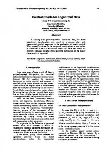
UCL = D= = 0.0492 R 4 * R 2.115*0.02324 Control Limits for X -Chart are obtained as:

CL= X= 74.00118 x LCL x = X − A2 * R = 74.00118 − 0.577 * 0.02324 = 73.98777

UCLx = X + A2 * R = 74.00118 − 0.577 * 0.02324 = 74.01459 By plotting the control limits, sample ranges and sample Consider the data given below in Table 3 is the Example 5.1 (Montgomery[10], page 213). The data is pertaining to means, one may get R − Chart and X − Chart as the manufacturing of Piston Rings for an auto motive engine given in Figure 3 and Figure 4. Fro m the R − Chart, we produced by a forging process. Twenty five samples, each of observe that all the plotted sample range values are falling size five have been taken and the inside d iameter is measured. within the control limits. Hence we may conclude that the The resulting data together with the sample means and variations are under control. Similarly fro m the X − Chart , sample range values are given below in Table 3. we observe that all the plotted sample means are falling Fro m the above values we have obtained the follo wing: inside the control limits. Hence we may conclude that the averages are also under the statistical control. , and R = 0 . 0232 X = 74.0011

3. Numerical Example

J. Subramani et al.: Control Charts for Variables with Specified Process Capability Indices

108

Table 3. Data of Inside Diameter of Piston Rings (Spec: 74.000±0.05 mm)

Range Values

Sample Number 1 2 3 4 5 6 7 8 9 10 11 12 13 14 15 16 17 18 19 20 21 22 23 24 25

x1 74.030 73.995 73.988 74.002 73.992 74.009 73.995 73.985 74.008 73.998 73.994 74.004 73.983 74.006 74.012 74.000 73.994 74.006 73.984 74.000 73.982 74.004 74.010 74.015 73.982

x2 74.002 73.992 74.024 73.996 74.007 73.994 74.006 74.003 73.995 74.000 73.998 74.000 74.002 73.967 74.014 73.984 74.012 74.010 74.002 74.010 74.001 73.999 73.989 74.008 73.984

x3 74.019 74.001 74.021 73.993 74.015 73.997 73.994 73.993 74.009 73.990 73.994 74.007 73.998 73.994 73.998 74.005 73.986 74.018 74.003 74.013 74.015 73.990 73.990 73.993 73.995 Average

x5 74.008 74.004 74.002 74.009 74.014 73.993 74.005 73.988 74.004 73.995 73.990 73.996 74.012 73.984 74.007 73.996 74.007 74.000 73.997 74.003 73.996 74.009 74.014 74.010 74.013

Sample Mean 74.0102 74.0006 74.0080 74.0030 74.0034 73.9956 74.0000 73.9968 74.0042 73.9980 73.9942 74.0014 73.9984 73.9902 74.0060 73.9966 74.0008 74.0074 73.9982 74.0092 73.9998 74.0016 74.0024 74.0052 73.9982 74.00118

Range R 0.038 0.019 0.036 0.022 0.026 0.024 0.012 0.030 0.014 0.017 0.008 0.011 0.029 0.039 0.016 0.021 0.026 0.018 0.021 0.020 0.033 0.019 0.025 0.022 0.035 0.02324

The manufacturing capability of a process can normally be

0.06 0.05 0.04 0.03 0.02 0.01 0.00

evaluated in terms of process capability indices

Cp

and

C pk . The process capability indices obtained from the above values are given below:

USL − LSL 74.05 − 73.95 = = 1.6681 6R / d2 6*0.2324 / 2.326

= Cp

1 3 5 7 9 11 13 15 17 19 21 23 25 LCL-R

R-Bar

UCL-R

Figure 3. R-Chart- Usual Method

Average Values

x4 73.992 74.011 74.005 74.015 73.989 73.985 74.000 74.015 74.005 74.007 73.995 74.000 73.997 74.000 73.999 73.998 74.005 74.003 74.005 74.020 74.005 74.006 74.009 74.000 74.017

= C pu

USL − X 74.05 − 74.00118 = = 1.6287 3R / d 2 3*0.2324 / 2.326

X − LSL 74.00118 − 73.95 = = 1.7075 3R / d 2 3*0.2324 / 2.326 = C pk Min = (C pu , C pl ) Min(1.6287,1.7075) = 1.6287

Range

C pl =

If the customer’s requirement of the process capability

Cp

74.03

index

74.02

capability indices that the process is an efficient one. However If the customer’s requirement of the process

is 1.5, then one may conclude fro m the above

Cp

74.01

capability index

74.00

above capability indices that the process is not an efficient one and hence the process has to be adjusted so as the

73.99

resulting process capability index

is 2.0, then one may conclude fro m the

Cp

is at least 2.0.

Case 2: Control Charts with specified C p = 1.5

73.98 1 3 5 7 9 11 13 15 17 19 21 23 25 S_ Mean

LCL

X-Bar

Figure 4. X-Bar Chart- Usual Method

UCL

In this case we construct the control limits for the given value of process capability index

C p and

hence separate

computation of the process capability index is not required. Further the proposed control charts states that the process is under the statistical control means that the process satisfies

International Journal of Probability and Statistics 2012, 1(4): 101-110

the requirement of the process capability index. Hence one can construct several control limits for different values of process capability index Cp . If any plotted points falls outside the control limits with specified Cp = 1.5 means that the process does not satisfy the required process capability index Cp = 1.5. Let the given process capability index Cp = 1.5. Then the Control limits for R − Chart with specified Cp = 1.5 are obtained as given below:

T  0.1  = CLR D= . 0.3877= 1.5  0.2585 Cp *

 0.1  * T = LCLR D= 0= 3 1.5  0 Cp  0.1  * T = UCLR D= 0.8199= 0.0547 4.  Cp 1.5  Control limits for X − Chart with specified C p = 1.5

CL= X= 74.00118 x LCLx = X − A2*.

T  0.1  74.00118 − 0.2159   = 73.9868 = Cp 1.5 

UCLx = X + A2*.

T  0.1  74.00118 + 0.2159   = 74.0156 = Cp 1.5 

109

values are falling within the control limits. Hence we may conclude that the variations are under control. Similarly fro m the X − Chart , we observe that all the plotted sample means are falling inside the control limits. Hence we may conclude that the averages are also under the statistical control. Further we conclude that the process capability index for the given p rocess is at least 1.5 and satisfies the customer’s requirements. Case 3: Control Charts with specified Cp =1.5 In this case we construct the control limits for the given value of process capability index Cpk and hence separate computation of the process capability index is not required. Further the proposed control charts states that the process is under the statistical control means, the process satisfies the requirement of the process capability index. Hence one can construct several control limits for different values of process capability index. If any p lotted points falls outside the control limits with specified Cpk=1.5 means that the process does not satisfy the required process capability index. Cpk=1.5. Let the given process capability index C p = 1.5. Further X = 74.00118 > M = 74.00 the control limits with specified process capability index Cpk=1.5 are obtained as given below: Control limits for R − Chart with specified Cpk value USL − X   74.05 − 74.00118  CLR= R= Dk*  = 0.775  = 0.025224 C 1.5  pk  

   74.05 − 74.00118  * USL − X = LCLR D= =  0 3k   0 1.5   C pk     74.05 − 74.00118  * USL − X = UCLR D=  1.64  = 4k   0.053377 1.5 C  pk  

Control limits for the proposed X − Chart with specified C pk = 1.5 value are obtained as given below:

CL= X= 74.00118 x Figure 5. R- Chart with Specified Cp=1.5

USL − X  LCLx= X − A2*k    C pk   74.05 − 74.00118  = 74.00118 − 0.432   1.5  = 73.98712

USL − X  UCLx= X + A2*k    C pk 

Figure 6. X-Bar Chart with Specified Cp=1.5

By plotting the control limits, sample ranges and sample means, one may get R − Chart and X − Chart with specified C p = 1.5 as given in Figure 5 and Figure 6. Fro m the R − Chart , we observe that all the plotted sample range

 74.05 − 74.00118  = 74.00118 + 0.432   1.5  = 74.01524 By plotting the control limits, sample ranges and sample means, one may get R − Chart and X − Chart with specified Cpk=1.5 as given in Figure 7 and Figure 8. Fro m the R − Chart , we observe that all the plotted sample range values are falling within the control limits. Hence we may conclude that the variations are under control. Similarly fro m the X − Chart ,

110

J. Subramani et al.: Control Charts for Variables with Specified Process Capability Indices

we observe that all the plotted sample means are falling inside the control limits. Hence we may conclude that the averages are also under the statistical control. Fu rther we conclude that the process capability index Cpk for the given process is at least 1.5 and satisfies the customer’s requirements.

ACKNOWLEDGEMENTS The authors are thankful to the editor and the referees for their useful co mments, which have helped to imp rove the presentation of the paper.

REFERENCES

Figure 7. R-Chart with Specified Cpk=1.5

Figure 8. X-Bar Chart with Specified Cpk=1.5

4. Conclusions In this paper, we have proposed a control chart which is based on the process capability indices Cp and Cpk for on line process control, which have the benefit of the usual control charts and the process capability ind ices. That is, the proposed control charts combines the two stage controlling mechanis m namely, Control Charts and the process capability indices into a single stage controlling mechanism to mon itor the process online and to assess the suitability of the manufacturing process. It has been shown that the relative performance of the p roposed control charts for variables can be assessed with that of usual variable control charts. It has also been shown that the proposed control chart is simple to apply and does not warrant any tedious computations both for control charts and for computing process capability indices. Moreover, we have also presented tables for the control charts constants for co mputing the control limits of the capability based control charts. The proposed method has also been illustrated with a numerical example. This study can also be extended to develop control charts based on other process capability indices.

[1]

Ashok Sarkar and Surajit Pal, “Process Control and Evaluation in the Presence of Systematic Assignable Cause”, Quality Engineering, Vol.10, pp.383-388, 1997

[2]

Balamurali, S, “Bootstrap Confidence Limits for Short Run Capability Indices”, Quality Engineering, Vol.15, pp.643-648, 2003

[3]

Balamurali, S., and Kalyanasundaram, M “BootstrapLower Confidence limits for the Process Capability Indices Cp, Cpk and Cpm ”, International Journal of Quality and Reliability M anagement, Vol. 19, No.8/9, pp.1088-1097, 2002

[4]

Bissell, A. F. “How Reliable is Your Capability Index?”, Applied Statistics, Vol.39, pp.331-340, 1990

[5]

Chou, Y., Owen, D.B., and Borrego, .A “Lower Confidence Limits on Process Capability Indices”, Journal of Quality Technology, Vol.22, pp.223-229, 1990

[6]

Franklin, L.A., and Wasserman, G.S. “Bootstrap Confidence Interval Estimates of Cpk: An Introduction”, Communications in Statistics - Simulation and Computation, Vol.20, pp.231-242, 1991

[7]

Franklin, L.A., and Wasserman, G.S. “Bootstrap Lower Confidence Limits for Process Capability Indices”, Journal of Quality Technology , Vol.24, No.4, pp.196-210, 1992

[8]

Kane, V. E., “ Process Capability Indices”, Journal of Quality Technology, Vol.18, pp.41-52, Corrigenda pp. 265, 1986

[9]

Kotz, S., and Johnson, N.L. “Process Capability Indices – A Review, 1992-2000”, Journal of Quality Technology, Vol.34, No.1, pp.2-19, 2002

[10] M ontgomery, D.C, Introduction to Statistical Quality Control, Fourth Edition, John Wily, New York, 2001 [11] Spring, F.A, “Assessing Process Capability in the Presence of Systematic Assignable Cause”, Journal of Quality Technology, Vol.23, pp.125-132, 1991. [12] Subramani, J, “Application of Systematic Sampling in Process Control, Statistics and Applications,” Journal of Society of Statistics, Computer and Applications, (New Series), 1, 7-17, 2004 [13] Subramani, J, “Process Control in the Presence of Linear Trend”, M odel Assisted Statistical Applications, 5, 272-281, 2010 [14] Subramani, J, Balamurali S, “On Line Computation of Process Capability Indices”, International Journal of Statistics and Applications, Vol2, no.5, 2012, To appear.