Joint 48th IEEE Conference on Decision and Control and 28th Chinese Control Conference Shanghai, P.R. China, December 16-18, 2009
FrC18.2
Control of Nonlinear Systems with Full State Constraint Using A Barrier Lyapunov Function Keng Peng Tee and Shuzhi Sam Ge Abstract— This paper presents a control for state-constrained nonlinear systems in strict feedback form to achieve output tracking. To prevent states from violating the constraints, we employ a Barrier Lyapunov Function, which grows to infinity whenever its arguments approaches some limits. By ensuring boundedness of the Barrier Lyapunov Function in the closed loop, we guarantee that the limits are not transgressed. We show that asymptotic output tracking is achieved without violation of state constraints, and that all closed loop signals are bounded, provided that some feasibility conditions on the initial states and control parameters are satisfied. Sufficient conditions to ensure feasibility are provided, and they can be checked offline by solving a static constrained optimization problem. The performance of the proposed control is illustrated through a simulation example.
I. I NTRODUCTION Constraints are ubiquitous in physical systems, and manifest themselves as physical stoppages, saturation, as well as performance and safety specifications, among others. Violation of the constraints during operation may result in performance degradation, hazards or system damage. Driven by practical needs and theoretical challenges, the rigorous handling of constraints in control design has become an important research topic in recent decades. To handle both state and input constraints in linear systems, many techniques have been developed, most of which are based on notions of set invariance using Lyapunov analysis [1], [2], [3]. Alternatively, Model Predictive Control considers the problem within an optimization framework inherently suitable for handling constraints, by solving an on-line finite horizon open-loop optimal control problem, subject to the system dynamics and constraints (see e.g. [4], [5]). In addition, reference governors have also been proposed to tackle the problem of constraints in nonlinear systems [6], [7]. For control of nonlinear systems in strict feedback form, the well known backstepping technique can be employed. Backstepping provides a systematic, recursive control design methodology that removes the restrictions of matching and growth conditions. Adaptive backstepping yields a means of applying adaptive control to parametric-uncertain systems [8], as well as systems with uncertain functions [9]. Although backstepping is considered a mature technique in the context This work is partially supported by A*Star SERC Grant No. 052-1010097. K. P. Tee is with the Institute for Infocomm Research, A*STAR, Singapore 138632
[email protected] S. S. Ge is with the Department of Electrical & Computer Engineering, National University of Singapore, Singapore 117576
[email protected]
978-1-4244-3872-3/09/$25.00 ©2009 IEEE
of strict feedback systems, there has been very few works that address, explicitly, the presence of constraints within this framework. A few exceptions are [10], in which nonovershooting tracking response for strict feedback systems is achieved, and [11], which presented modified backstepping based on positively invariant feasibility regions for a class of nonlinear systems with control singularities. In this paper, we employ a Barrier Lyapunov Function to tackle the issue of constraint. The proposed method exploits the property that a barrier function grows to infinity whenever its arguments approaches some limits. By keeping the Barrier Lyapunov Function bounded in the closed loop system, it is thus guaranteed that the barriers are not transgressed. Barrier functions have been used to design controllers for systems in Brunovsky form [12], strict feedback form [13], output feedback form [14], as well as for electromagnetic oscillators [15] and electrostatic microactuators [16]. We extend the work of [13], on strict feedback systems with an output constraint, to the more difficult problem wherein constraints are present in all of the states. Unlike [13], [16], in which only the first step of the backstepping design involves the use of a barrier function, we employ a barrier function for each step of backstepping design to deal with the full state constraint in this paper. Canceling of cross coupling terms is accommodated, and post-design analysis reveal that the stabilizing functions and control remain bounded. We formulate sufficient conditions to determine a priori if the proposed control is feasible, and they can be check offline by solving a static constrained optimization problem. The remainder of this paper is organized as follows. In Section II, we formulate the problem of tracking control for nonlinear strict feedback systems with constraints in the states, and provide an exposition of the main ideas underlying the use of barrier Lyapunov functions for constraint satisfaction. Following that, in Section III, we present the control design to ensure that each state of the plant is constrained, and provide feasibility conditions in terms of the design parameters, the constraints, and the initial conditions. Section IV shows how to perform an offline check of the feasibility conditions by casting it as a static constrained optimization problem. The simulation study in Section V illustrates the performance of the control, and Section VI presents concluding remarks. II. P ROBLEM F ORMULATION AND P RELIMINARIES Throughout this paper, we denote by R+ the set of nonnegative real numbers, and k • k the Euclidean vector norm in Rm . A semicolon “;” in function argument indicates that
8618
FrC18.2 any symbols that follow represent parameters, e.g. f (x; k) denotes the value of the function f at x with parameter k. The symbols λmax (•) and λmin (•) denote the maximum and minimum eigenvalues of •, respectively. We also denote x ¯i = [x1 , x2 , ..., xi ]T , z¯i = [z1 , z2 , ..., zi ]T , and y¯di = (1) (2) (i) [yd , yd , ..., yd ]T . Consider the following nonlinear system in strict feedback form: x˙ i x˙ n
= =
fi (¯ xi ) + gi (¯ xi )xi+1 , fn (¯ xn ) + gn (¯ xn )u
y
=
x1
Vi
i = 1, 2, ..., n − 1 -kb i
(1)
where f1 , ..., fn , g1 , ..., gn are smooth functions, x1 , ..., xn are the states, u and y are the input and output respectively. We consider the problem of full state constraint, that is, xi (t) is required to remain in the set |xi | ≤ kci ∀t > 0, with kci a positive constant, for all i = 1, ..., n. The control objective is to track a desired trajectory yd while ensuring that all closed loop signals are bounded and that the state constraints are not violated. Note that the state constraints are not necessarily physical constraints but can also be performance requirements. Assumption 1: For any kc1 > 0, there exist positive constants A0 , Y1 , Y2 ,..., Yn such that the desired trajectory i yd (t) and its time derivatives y (i) d (t) := ddtyi , i = 1, ..., n satisfy |y (i) d (t)| < Yi ,
|yd (t)| ≤ A0 < kc1 ,
i = 1, ..., n
=
h(t, z)
(3)
where h : R+ × N → Rn is piecewise continuous in t and locally Lipschitz in z, uniformly in t, on R+ × Z. Let Zi := {zi ∈ R : |zi | < kbi } ⊂ R. Suppose that there exist
kb i
zi
Schematic illustration of a Barrier Lyapunov Function.
positive definite functions Vi : Zi → R+ (i = 1, ..., n), continuously differentiable on Zi , and they satisfy Vi (zi ) → ∞ as zi → ±kbi
(4)
where γ1 and γ2 are class K∞ functions. Let V (η) := P n i=1 Vi (zi ), and zi (0) ∈ Zi , i = 1, ..., n. If the inequality holds: ∂V V˙ = h ≤ 0 ∂z
(2)
for all t ≥ 0. Assumption 2: The functions gi (¯ xi ), i = 1, 2, ..., n, are known, and there exists a positive constant g0 such that 0 < g0 ≤ |gi (¯ xi )| for |xj | < kcj , j = 1, 2, ..., i. Without loss of generality, we further assume that the gi (¯ xi ), i = 1, 2, ..., n, are all positive for |xj | < kcj , j = 1, 2, ..., i. Definition 1: [13] A Barrier Lyapunov Function is a scalar function V (x), defined with respect to the system x˙ = f (x) on an open region D containing the origin, that is continuous, positive definite, has continuous first-order partial derivatives at every point of D, has the property V (x) → ∞ as x approaches the boundary of D, and satisfies V (x(t)) ≤ b ∀t ≥ 0 along the solution of x˙ = f (x) for x(0) ∈ D and some positive constant b. A schematic illustration of a Barrier Lyapunov Function is provided in Figure 1. The following lemma formalizes the result for general forms of barrier functions in Lyapunov synthesis satisfying Vi (zi ) → ∞ as |zi | → kbi , and is used to ensure that the state constraints are not violated. Lemma 1: For any positive constants kbi , i = 1, 2, ..., n, let Z := {z ∈ Rn : |zi | < kbi , i = 1, 2, ..., n} ⊂ Rn be an open set. Consider the system z˙
Fig. 1.
0
(5)
then zi (t) ∈ Zi ∀t ∈ [0, ∞). Proof: Since the right hand side of (3) is piecewise continuous in t and locally Lipschitz in z, uniformly in t, on R+ × Z, existence and uniqueness of the solution η(t) is ensured on a time interval [0, τmax ), as follows from [17, p.476 Theorem 54]. From the fact that zi (0) ∈ Zi , i = 1, ..., n, we know that Vi (zi (0)), i = 1, ..., n, and thus V (z(0)), exist. Since V (z) is positive definite and V˙ ≤ 0, we knowP that V (z(t)) ≤ n V (z(0)) ∀t ∈ [0, τmax ). From V (z) = i=1 Vi (zi ) and the fact that Vi (zi ), i = 1, ..., n are positive functions, it is clear that each Vi (zi (t)) is bounded ∀t ∈ [0, τmax ). Since Vi (zi ) → ∞ only if zi → ±kbi , we conclude, from the boundedness of Vi (zi (t)), that |zi (t)| < kbi ∀t ∈ [0, τmax ). Therefore, there is a compact subset K ⊆ Z such that the maximal solution of (3) satisfies z(t) ∈ K ∀t ∈ [0, τmax ). According to [17, p.481 Proposition C.3.6], we conclude that z(t) is defined ∀t ∈ [0, ∞). It follows that |zi (t)| ∈ Zi ∀t ∈ [0, ∞). To establish asymptotic convergence of the signals to zero, we analyze the continuity properties of the derivative of the Lyapunov function candidate in the closed loop and use the following lemma. Lemma 2: [18] (Barbalat’s Lemma) Consider a differentiable function h(t). If limt→∞ h(t) is ˙ finite and h˙ is uniformly continuous, then limt→∞ h(t) = 0.
8619
FrC18.2 The following lemma is useful for computing the bounds of stabilizing functions αi within a compact set to check the feasibility conditions for state constraint problem. Lemma 3: For any positive constants κi and kbi , the following inequality holds for all zi in the interval |zi | ≤ kbi :
where kb1 = kc1 − A0 , and kbi , i = 2, ..., n, are positive constants to be determined from subsequent feasibility analysis. Note that V is positive definite and continuously differentiable in the set |zi | < kbi for all i = 1, 2, ..., n. Design the stabilizing functions and control law as
2 |(kb2i − zi2 )κi zi | ≤ √ κi kb3i (6) 3 3 2 2 Proof: Denote pi (zi ) := (kbi − zi )κi zi . The maximum value of pi (zi ) in the interval |zi | ≤ kbi is obtained at the stationary points or the boundary points. The stationary points of pi (zi ) are obtained from the equation: dpi = κi (kb2i − 3zi2 ) = 0 dzi k
(7)
k
which yields zi = √b3i and zi = − √b3i , both of which lies within the interval |zi | ≤ kbi . The corresponding values of pi (zi ) at these stationary points are, respectively: 2 pi = √ κi kb3i 3 3
2 and pi = − √ κi kb3i 3 3
z˙1 z˙i
(8) z˙n (9)
Taking into account both stationary and boundary points, it is clear that 2 (10) |pi | ≤ √ κi kb3i 3 3 and thus, inequality (6) holds.
i=1
Vi ,
Vi =
k2 1 log 2 bi 2 , 2 kbi − zi
=
u
=
−(kb21 − z12 )κ1 z1 + g1 z2 (15) 2 2 k − zi = −(kb2i − zi2 )κi zi − 2 bi 2 gi−1 zi−1 kbi−1 − zi−1 +gi zi+1 (16) 2 2 k − zn gn−1 zn−1 = −(kb2n − zn2 )κn zn − 2 bn 2 kbn−1 − zn−1 (17) =
The time derivative of V along (15)-(17) can be rewritten as V˙ = −
n X
κj zj2
(18)
j=1
z˙ = h(t, z)
For the problem of output constraint tackled in [13], only the first step of the backstepping design involves the use of a barrier function. By enforcing a constraint on the output tracking error z1 = y −yd , the output y is constrained within a specified zone, provided that the desired trajectory yd is also within the same zone. In this paper, we consider the case of full state constraints, and extend the use of barrier functions to every step, in order to keep each error signal zi = xi − αi−1 (i = 2, ..., n) constrained. Provided that each stabilizing function αi−1 is bounded in the specified constrained region for xi , we can ensure that xi remains in the constrained region. In view of this, state constraints cannot be arbitrarily specified, but are subject to feasibility conditions, based on the stabilizing functions αi−1 designed via backstepping with a Barrier Lyapunov Function. Nevertheless, the feasibility conditions can be checked a priori to determine if the given problem can be solved under this approach. Denote z1 = x1 − yd and zi = xi − αi−1 , i = 2, ..., n. Consider the Lyapunov function candidate: n X
αi
1 (12) (−f1 − (kb21 − z12 )κ1 z1 + y˙ d ) g1 1 (−fi + α˙ i−1 − (kb2i − zi2 )κi zi gi k 2 − zi2 i = 2, ..., n (13) − 2 bi 2 gi−1 zi−1 ), kbi−1 − zi−1 αn (14)
Let the closed loop system (15)-(17) be written as
III. BACKSTEPPING D ESIGN W ITH A BARRIER LYAPUNOV F UNCTION
V =
=
where κi , i = 1, ..., n, are positive constants. This yields the closed loop system
At the boundary points |zi | = ±kbi , we have that pi = 0
α1
i = 1, ..., n
(19)
where h(t, z) is piecewise continuous in t and locally Lipschitz in z, uniformly in t, on z ∈ Z := {z ∈ Rn : |zi | < kbi , i = 1, 2, ..., n}. Hence, from (18) and Lemma 1, we have that |zi (t)| < kbi for all t > 0 and i = 1, ..., n, provided that |zi (0)| < kbi . Remark 1: From (13), there appears to be a possibility of αi becoming unbounded if zi−1 (t) = kbi−1 at some t, and the propagation of the derivatives of αi , down to the design of control u in the final step of backstepping, 2 releases even more terms comprising (kb2i−1 − zi−1 ) in the denominator. This issue is addressed in Theorem 1, where it will be formally shown that, in the closed loop, under some initial and feasibility conditions, the magnitude of the error signals zi−1 (t) are bounded away from kbi−1 ∀t > 0, thus ensuring that the stabilizing functions α2 , ..., αn−1 and control u remain bounded. Theorem 1: Consider the closed loop system (1), (12)(14) under Assumptions 1-2. Let ξ = [κ1 , ..., κn−1 , kb2 , ..., kbn ]T be the control parameters, and Ai (ξ) be an upper bound for αi in compact set Ωi , parameterized by ξ:
(11)
8620
Ai (ξ) ≥
sup (¯ xi , z¯i , y¯di ) ∈ Ωi
|αi (¯ xi , z¯i , y¯di ; ξ)| i = 1, ..., n − 1
(20)
FrC18.2 Ω1 , and thus, the stabilizing function α1 (x1 , z1 , y¯d1 ) in (12) is bounded since it is a continuous function. As a result, sup(x1 , z1 , y¯d )∈ Ω1 |α1 (x1 , z1 , y¯d1 )| exists, and 1 an upper bound A1 can be found. Then, from |z2 (t)| ≤ Dz2 < kb2 , we can show that
where Ωi
:=
{¯ xi ∈ Ri , z¯i ∈ Ri , y¯di ∈ Ri :
(j)
|xj | ≤ Dzj + Aj−1 , |zj | ≤ Dzj , |yd | ≤ Yj ,
Dzj
:=
j = 1, ..., i} s Πn (k 2 − z 2 (0)) kbj 1 − k=1 nbk 2 k Πk=1 kbk
(21)
Given the constraints kci+1 > 0, i = 1, ..., n − 1, and that the following conditions hold: C1) there exist positive constants κ1 , ..., κn−1 , kb2 , ..., kbn such that kci+1
> Ai (ξ) + kbi+1
(23)
for all i = 1, ..., n − 1. C2) the initial conditions z¯n (0) belong to the set zn ∈ Rn : |zi | < kbi , i = 1, 2, ..., n} Ωz0 := {¯
(24)
then the following properties hold. i) The signals zi (t), i = 1, 2, ..., n, remain in the compact set defined by Ωz = {¯ zn ∈ Rn : |zi | ≤ Dzi , i = 1, 2, ..., n}. ii) Every state xi (t) remains in the set Ωx := {¯ xn ∈ Rn : |xi | ≤ Dzi + Ai−1 < kci , i = 1, ..., n} ∀t > 0, i.e. the full state constraint is never violated. iii) All closed loop signals are bounded. iv) The output tracking error z1 (t) converges to zero asymptotically, i.e., y(t) → yd (t) as t → ∞. Proof: i) From the fact that V˙ ≤ 0, it is clear that V (t) ≤ V (0). Since zi2 (0) < kb2i from Condition C2, it is straightforPn k2 ward to obtain that V (0) ≤ i=1 12 log k2 −zbi2 (0) which i bi implies that k2 1 log 2 bi 2 2 kbi − zi
≤
n X 1 j=1
2
log
kb2j kb2j
−
zj2 (0)
kb2i 2 kbi − zi2
≤
log
Πnj=1 kb2j Πnj=1 (kb2j − zj2 (0))
(26)
for i = 1, ..., n. Furthermore, we know, from Lemma 1, that kb2i − zi2 (t) > 0 ∀ t > 0. Then, the above can be rearranged to yield |zi (t)| ≤ Dzi ∀ t > 0. ii) Since |z1 (t)| ≤ Dz1 < kc1 − A0 , we can show that |x1 (t)| ≤ Dz1 + |yd (t)| < kc1 − A0 + |yd (t)|
(27)
Noting that |yd (t)| ≤ A0 from Assumption 1, we therefore conclude that |x1 (t)| ≤ Dz1 + A0 < kc1 , ∀ t > 0. To show that |x2 (t)| ≤ kc2 , we need to first verify that there exists a positive constant A1 such that |α1 (t)| ≤ A1 , ∀ t > 0. Since |x1 (t)| ≤ Dz1 + A0 , |z1 (t)| ≤ Dz1 , and |y˙ d (t)| ≤ Y1 , it is clear that (x1 (t), z1 (t), y¯d1 (t)) ∈
(28)
Since |α1 (t)| ≤ A1 , we conclude that |x2 (t)| ≤ Dz2 + A1 < kb2 + A1 < kc2 , ∀ t > 0. We can progressively show that |xi+1 (t)| ≤ kci+1 , i = 2, ..., n − 1, after verifying that there exist positive constants Ai such that |αi (t)| ≤ Ai , ∀ t > 0. Since (i) |xi (t)| ≤ Dzi + Ai−1 , |zi (t)| ≤ Dzi , and |yd (t)| ≤ Yi , it is clear that (¯ xi (t), z¯i (t), y¯di (t)) ∈ Ωi , and thus, the stabilizing function αi (¯ xi , z¯i , y¯di ) in (12) is bounded since it is a smooth function. As a result, we have that sup(¯xi , z¯i , y¯d )∈ Ωi |αi (¯ xi , z¯i , y¯di )| exists, and an i upper bound Ai can be found. Then, from |zi+1 (t)| ≤ Dzi+1 < kbi+1 , we can show that |xi+1 (t)| ≤ Dzi+1 + |αi (t)| < kbi+1 + |αi (t)|. Since |αi (t)| ≤ Ai , we conclude that |xi+1 (t)| ≤ Dzi+1 + Ai < kbi+1 + Ai < kci+1 , ∀ t > 0. iii) By inspection of the stabilizing functions αi (¯ xi , z¯i , y¯di ) and control u(¯ xn , z¯n , y¯dn ) , it is clear that they are bounded, by virtue of the boundedness of x ¯n (t), z¯n (t), y¯dn (t), and, in particular, by |zi (t)| ≤ Dzi < kbi , which prevents any term comprising (kb2i − zi2 (t)) in the denominator from becoming unbounded. iv) Based on (15), (16), and (17), and the fact that |xi (t)| ≤ kci , |zi (t)| ≤ Dzi , i = 1, ..., n, it can be shown that V¨ (t) is bounded, thus implying that V˙ (t) is uniformly continuous. Then, by Lemma 2, we obtain that zi (t) → 0 as t → ∞. Since z1 (t) = x1 (t) − yd (t) and y(t) = x1 (t), it is clear that y(t) → yd (t) as t → ∞. IV. F EASIBILITY C HECK
(25)
for i = 1, ..., n. Using the identity log a+log b = log ab, we rewrite the above into the following log
|x2 (t)| ≤ Dz2 + |α1 (t)| < kb2 + |α1 (t)|
(22)
By a feasibility check, we are referring to the question: For a given initial condition, does there exist a set of design parameters for the control (14) such that output tracking is achieved without violating any of the state constraints? In some cases, when the states are to be constrained in a small set, such a control may not exist. In this paper, we formulate the feasibility conditions C1 and C2, which are sufficient conditions to achieve output tracking in the presence of state constraints. In particular, ensuring that C1 is met ensures that the state constraints |xi (t)| < kci are also met, since |zi (t)| < kbi is ensured by our proposed control based on a Barrier Lyapunov Function. However, if C1 and C2 cannot be met, we cannot make any conclusions on the feasibility of the problem. The feasibility conditions depend on the state constraints, the initial conditions and the design parameters κ1 , ..., κn−1 , kb2 , ..., kbn . Since the state constraints are specified and the initial conditions cannot be chosen, this amounts to the search for a set of design parameters that satisfies the feasibility conditions, if it exists. We favor the parameters
8621
FrC18.2 κi , i = 1, ..., n − 1, to be large in order to achieve rates Phigh n of error convergence, as follows from V˙ = − j=1 κj zj2 . The values of kbi , i = 2, ..., n, should also be large, so as to enlarge the set of feasible initial conditions according to |zi (0)| < kbi . However, the feasibility conditions C1 and C2 impose upper bounds on the design parameters. These tradeoffs can be formulated as a static nonlinear constrained optimization problem that can be solved offline, prior to actual implementation. Specifically, we check if there exists a solution ξ := [κ1 , ..., κn−1 , kb2 , ..., kbn ]T for the optimization problem: max
κ1 ,...,κn−1 ,kb2 ,...,kbn >0
subject to:
P (ξ) =
n−1 X
κi +
i=1
n X
k bi
i=2
kci+1 > Ai (ξ) + kbi+1 xi (0), z¯i (0), y¯di (0); ξ)| kbi+1 > |xi+1 (0) − αi (¯ i = 1, ..., n − 1 (29) where P is the objective function. If a solution ξ ∗ to the above optimization problem exists, then C1 and C2 in Theorem 1 are satisfied, and the proposed control (14) with ξ = ξ ∗ is feasible in ensuring output tracking for (1) while respecting the full state constraint for all time. V. S IMULATION In this section, we present simulation studies to illustrate the performance of the proposed control. Consider the following second-order nonlinear system x˙ 1 x˙ 2
= 0.1x21 + x2 = 0.1x1 x2 − 0.2x1 + (1 + x21 )u
(30)
The objective is for x1 to track desired trajectory yd , subject to full state constraint |x1 | < kc1 = 0.8 and |x2 | < kc2 = 2.5. For simplicity, we consider that yd ≡ 0, i.e., a stabilization task. First we provide a step by step description for the design of the control law. For illustration, consider the initial states x1 (0) = −0.45 and x2 (0) = −1.95. Denote ξ = [κ1 , kb2 ]T . Step 1: Determine A0 , Y1 , upper bounds for |yd (t)| and |y˙ d (t)| respectively, according to Assumption 1. Since yd ≡ 0, we have A0 = Y1 = 0. Step 2: Compute kb1 = kc1 − A0 = 0.8, and check that |z1 (0)| < kb1 is satisfied. Step 3: Compute α1,0 (ξ) := α1 (x1 (0); ξ) from (12) as: α1,0 (ξ) = −0.0203 + 0.1969κ1
(31)
Step 6: Find a solution ξ ∗ = [κ∗1 , kb∗2 ]T , if it exists, of the static optimization problem (29): max P := κ1 + kb2
κ1 ,kb2 >0
(34)
subject to the constraints kc2
> A1 (ξ) + kb2
kb 2
> | − 1.95 − α1,0 (ξ)|
(35)
Using the Matlab routine fmincon.m, we obtain κ∗1 = 1.285 and kb∗2 = 2.183. Step 7: Select any κ2 > 0 and implement the control law u(¯ x2 ; ξ ∗ ) in (14). In this study, we let κ2 = 4. The above steps are repeated for various initial states in the state space x1 ∈ [−0.75, 0.75], x2 ∈ [−2.45, 2.45]. If a point yields a solution ξ ∗ in Step 6, then it is labeled with an ‘o’ to indicate that it is feasible. Otherwise, it is labeled with an ‘x’. Figure 2 shows that nearly all the points in the tested set are feasible. The closed loop state trajectories, starting from various initial conditions, are shown in Figure 3. The initial conditions are indicated by ‘+’. The trajectories converge to the origin and satisfy the state constraint requirements |x1 | < kc1 and |x2 | < kc2 for all time, although the scale of the figure makes it difficult to tell the former condition. Figure 4 provides close up views of the closed loop state trajectories show that |x1 | < kc1 at all times despite approaching the constraint very closely. Figure 5 shows that output tracking is achieved. From various initial conditions, the tracking error z1 converges to zero. Furthermore, never does it transgress the limits at z1 = ±0.8. VI. C ONCLUSIONS In this paper, we have designed a control for strict feedback nonlinear systems with state constraints, using a Barrier Lyapunov Function. We have shown that asymptotic tracking is achieved without violation of the constraints, and that all closed loop signals remain bounded, under some feasibility conditions which involve the initial states and some design parameters. Although feasibility is not guaranteed for an arbitrary set of state constraints, we have presented a method of checking the feasibility and determining appropriate design parameters prior to implementing the control, by solving a static constrained optimization problem offline. Finally, we have illustrated the performance of the proposed control with a simulation example.
Step 4: Obtain Dz1 (ξ) from (22) as s 0.6836(kb22 − (−1.95 − α1,0 (ξ))2 ) Dz1 = 0.8 1 − kb22 (32) Step 5: With the help of Lemma 3, let A1 (ξ) be 2 A1 (ξ) := 0.1(Dz1 (ξ) + A0 )2 + Y1 + √ kb31 κ1 (33) 3 3
8622
R EFERENCES [1] D. Liu and A. N. Michel, Dynamical Systems with Saturation Nonlinearities. London, U.K.: Springer-Verlag, 1994. [2] T. Hu and Z. Lin, Control Systems With Actuator Saturation: Analysis and Design. Boston, MA: Birkhuser, 2001. [3] F. Blanchini, “Set invariance in control,” Automatica, vol. 35, pp. 1747–1767, 1999. [4] D. Q. Mayne, J. B. Rawlings, C. V. Rao, and P. O. M. Scokaert, “Constrained model predictive control: Stability and optimality,” Automatica, vol. 36, pp. 789–814, 2000.
FrC18.2
3
2
2
2
1
1
1
−1
x
0
x
x2
0
2
3
2
3
0
−1
−1
−2
−2
−2
−3 −3 −1
−0.8 −0.5
0 x1
0.5
1
−0.79 x
−3 0.785 0.79 0.795 0.8 0.805 x
−0.78
1
Most of the initial states in constrained state space satisfy the feasibility conditions C1 and C2. These are labeled with ‘o’. Those labeled with ‘x’ do not satisfy the feasibility conditions. Fig. 2.
1
Close up views show that the closed loop state trajectories are bounded away from the left and right limits of the constrained state space.
Fig. 4.
0.8 3 0.6 2
0.4 0.2
x
2
z
1
1
0
0 −0.2 −1 −0.4 −0.6
−2
−3 −1
−0.8 0 −0.5
0 x
0.5
1
0.5
1
1.5
2 t
2.5
3
3.5
4
1
The closed loop state trajectories, starting from various initial conditions marked by ‘+’, converge to the origin and remain in the interior of the rectangle constraint for all time.
Fig. 3.
[5] F. Allg¨ower, R. Findeisen, and C. Ebenbauer, “Nonlinear model predictive control,” Encyclopedia of Life Support Systems (EOLSS) article contribution 6.43.16.2, 2003. [6] E. G. Gilbert, I. Kolmanovsky, and K. T. Tan, “Nonlinear control of discrete-time linear systems with state and control constraints: A reference governor with global convergence properties,” in Proc. 33rd IEEE Conf. Decision & Control, (Orlando, FL), pp. 144–149, 1994. [7] E. G. Gilbert and I. Kolmanovsky, “Nonlinear tracking control in the presence of state and control constraints: a generalized reference governor,” Automatica, vol. 38, pp. 2063–2073, 2002. [8] M. Krstic, I. Kanellakopoulos, and P. V. Kokotovic, Nonlinear and Adaptive Control Design. New York: Wiley and Sons, 1995. [9] S. S. Ge and C. Wang, “Adaptive neural control of uncertain MIMO nonlinear systems,” IEEE Trans. Neural Networks, vol. 15, no. 3, pp. 674–692, 2004. [10] M. Krstic and M. Bement, “Nonovershooting control of strict-feedback nonlinear systems,” IEEE Trans. Automatic Control, vol. 51, no. 12, pp. 1938–1943, 2006. [11] Z. H. Li and M. Krstic, “Maximizing regions of attraction via backstepping and CLFs with singularities,” Systems & Control Letters, vol. 30, pp. 195–207, 1997.
Fig. 5. Tracking errors for different initial conditions converge to zero while satisfying the constraint |z1 | < 0.8.
[12] K. B. Ngo, R. Mahony, and Z. P. Jiang, “Integrator backstepping using barrier functions for systems with multiple state constraints,” in Proc. 44th IEEE Conf. Decision & Control, (Seville, Spain), pp. 8306–8312, December 2005. [13] K. P. Tee, S. S. Ge, and E. H. Tay, “Barrier Lyapunov Functions for the control of output-constrained nonlinear systems,” Automatica, vol. 45, no. 4, pp. 918–927, 2009. [14] B. Ren, S. S. Ge, K. P. Tee, and T. H. Lee, “Adaptive control for parametric output feedback systems with output constraint,” in Proc. 48th IEEE Conf. Decision and Control, (Shanghai, China), 2009. [15] H. S. Sane and D. S. Bernstein, “Robust nonlinear control of the electromagnetically controlled oscillator,” in Proc. American Control Conference, (Anchorage, AK), pp. 809–814, May 2002. [16] K. P. Tee, S. S. Ge, and E. H. Tay, “Adaptive control of electrostatic microactuators with bidirectional drive,” IEEE Trans. Control Systems Technology, vol. 17, no. 2, pp. 340–352, 2009. [17] E. D. Sontag, Mathematical Control Theory. Deterministic FiniteDimensional Systems, Volume 6 of Texts in Applied Mathematics, Second edition. New York: Springer-Verlag, 1998. [18] J. E. Slotine and W. Li, Applied Nonlinear Control. Englewood Cliff, NJ: Prentice-Hall, 1991.
8623