Printed in the Netherlands. dynamics.tex; 30/03/2001; 9:26; p.1 ... To represent these situations Milord II provides the knowledge engineer with two ..... GÐdel's and Lukasiewicz's semantics (truth-tables) for finitely-valued logics [5, 6, 8, 7]. ...... Using Brewka's approach, the previous statements are represented as follows.
Control techniques for complex reasoning: The case of Milord II. Llu´ıs Godo, Josep Puyol-Gruart and Carles Sierra IIIA, Artificial Intelligence Research Institute. CSIC, Spanish Scientific Research Council. Campus UAB, 08193. Catalonia, Spain. ({godo, puyol, sierra}@iiia.csic.es) Abstract. In this paper we survey Milord II—a KBS design tool. We concentrate on its object level and meta-level languages, with special emphasis on the control techniques and the communication between both languages. The control, declarative in nature, is based on reflection techniques over a meta-language equipped with a declarative backtracking mechanism. Reflection and subsumption techniques are used to tackle the problem of knowledge incompleteness. This meta-level approach is based on assumptions over the current state of the object deductive process. Reflection makes meta-level deduction effective at the object level. Whenever the assumptions made at the meta-level are proved to be erroneous, a declarative backtracking mechanism retracts them. The deductive calculus at the object level is based on a rule specialization calculus. Complex reasoning tasks can be implemented using a combination of the overall set of Milord II meta-control techniques. To illustrate the use of such modelling techniques we present first a scheduling reasoning system, second a method for solving a general class of default reasoning problems, and finally a legal reasoning problem involving default rules and priorities. Keywords: Knowledge-based systems, Complex reasoning control.
1. Introduction Reasoning patterns occurring in complex problem solving tasks usually cannot be modelled by means of just a pure classical logic approach. This is due to several reasons, for instance: incompleteness of the available information, need of using and representing uncertain or imprecise knowledge, or combinatorial explosion of classical theorem proving when knowledge bases become large. To deal with these problems, Milord II, an architecture for Knowledge Base Systems (KBS), combines modularization techniques with both implicit and explicit control mechanisms and with an approximate reasoning component based on many-valued logics. Roughly speaking, a Knowledge Base (KB) in Milord II consists of a hierarchy of modules interconnected by their export interfaces. Each module contains an Object Level Theory (OLT) and a Metac 2001 Kluwer Academic Publishers. Printed in the Netherlands.
dynamics.tex; 30/03/2001; 9:26; p.1
2 Level Theory (MLT) interacting through a reflective mechanism (see Figure 1).
- Export
OLT 6? �
Import
Import
@ Export Export � M LT I @ @ ··· OLT OLT 6 ? M LT �
···
�
Import
6
? M LT
@ I @
�
···
I @ @
Figure 1. Structure of a Milord II module hierarchy.
A module can be understood as a functional abstraction between the set of components it needs as input and the type of results it can produce. From the logical point of view, Milord II makes use of both many-valued logic and epistemic meta-predicates to express the truth status of propositions. For further details in these logical topics the reader is referred to [4, 10, 11, 12, 13, 14]. In this chapter we focus on the control techniques used in Milord II that determine a KBS execution. The explicit part of the control, declarative in nature, is mainly based on a reflective approach and a declarative backtracking mechanism. In this context, reflection makes sense as a control mechanism because there is a clear separation between domain (object-level) and control (meta-level) knowledge. The basic implicit control components are a subsumption mechanism and a process of elimination of unnecessary rules, both concerning the object level. Next we list the most usual control requirements for a KBS language together with the solutions adopted in Milord II. Locality of Control: All explicit control mechanisms are specified locally to each module. This allows us to identify a module as the complete description of a problem (or subproblem). The separation between domain and control knowledge is a typical characteristic of most KBS languages to offer a clear and declarative programming style.
dynamics.tex; 30/03/2001; 9:26; p.2
3 Specificity versus generality: To solve problems, human experts are able to reason at different levels of precision depending on the amount of data at hand. For instance, a physician cannot always gather all the relevant data to make a complete and accurate diagnosis. This is the case, for example, when a patient is in a coma and thus the physician cannot pose him any question. Nonetheless, the physician has to make a diagnosis, although it may be provisional. To represent these situations Milord II provides the knowledge engineer with two different control options: −
To write rules with different levels of specificity (using more or less information, that is, putting more or less conditions) deducing the same conclusion with possibly different levels of belief. To deal with this kind of rules, Milord II extends the concept of subsumption by associating sets of partial labels to the rules. This technique guarantees the use of the more specific knowledge whenever possible.
−
To encode default-like rules (by means of meta-rules) that generate plausible assumptions to be used when a piece of relevant information is missing (see Section 9).
Avoidance of unnecessary work: Milord II takes advantage of the specialization deductive mechanism [10, 11] to eagerly detect when a rule cannot increase the certainty on a conclusion. When a rule is applied, Milord II’s engine decides whether other rules with the same conclusion can increase its certainty or not. If not, they are removed. Locality of threshold: In some cases knowledge engineers are interested in programming modules whose deduced predicates are only useful if their certainty is above a minimum truth level. This is done by declaring a threshold local to each module. Whenever a rule gets, by specialization, a truth interval with its minimum value below the module threshold, it is removed. Flexibility in data gathering: Given a query to a module, different strategies for the module to get an answer can be used. The different evaluation strategies of Milord II determine how and in which order the necessary external information is gathered. Declarativity of Control: Milord II Horn-like meta-rules are used as a declarative language to implement several control actions, e.g. elimination of rules, generation of plausible assumptions, dynamic changing of the modules hierarchy or dynamic creation of modules.
dynamics.tex; 30/03/2001; 9:26; p.3
4 The detailed description of the different implicit and explicit control mechanism of Milord II is structured in this Chapter as follows. In Section 2 we present a general picture of the whole control structure. Sections 3 through 8 are devoted to describe the different Milord II control mechanisms, that is, the object level process, the upwards reflection operation, the meta-level process, the downwards reflection operation and the communication among modules respectively. In Section 9 two reasoning tasks are implemented using some of the previously presented control mechanisms.
2. Milord II overview A Milord II KB consists of a hierarchy of modules, each module containing different kinds of knowledge, structured as sketched in Figure 2. From a logical point of view, a module is composed of an Object Level Theory (OLT) and a Meta Level Theory (MLT). The OLT is generated by a set of rules which are specified in the Deductive Knowledge definition. These rules are formulas belonging to the Object Level Language OLn , a propositional language based on many-valued semantics. Formulas of this language are of the form (r, V ), where r is a Hornlike rule and V is an interval of truth values belonging to a finite and totally ordered set of values, also specified in the module declaration. Deduction in the object level language, denoted `O , is mainly based on a specialization inference rule, a straightforward generalization of the many-valued version of Modus Ponens, which allows to simplify rules as soon as we know truth-intervals for any of their conditions. On the other hand, the MLT is generated by a set of meta-rules which are specified in the Deductive Control definition. These meta-rules are formulas of the Meta Level Language MLn , a restricted first order classical language of Horn rules. Variables in meta-rules, if any, are considered universally quantified. Deduction at the meta level, denoted by `M , is based on Modus Ponens and particularization. The overall reasoning process of a module consists on reasoning at each level and interacting between both levels. This process produces a sequence of modifications over the initial OLT and MLT. For a deeper insight of Milord II modules, the reader is again referred to [4, 14]. From an operational point of view, a module can be identified with a process attached to it, used to compute values (truth intervals) for all the propositions and variables contained in its export interface. Namely, a module execution consists of the reasoning process necessary to compute the values for the propositions and variables in the export interface the user queries about. The execution of a module can possibly
dynamics.tex; 30/03/2001; 9:26; p.4
5 activate the execution of submodules in the hierarchy. These executions only interact with the parent module through the export interface of the submodules, giving formulas back as result. It is worth noticing that the interaction is made only at the object level. Begin Hierarchy of submodules Import: ... Export: ... Deductive knowledge Dictionary: ... Rules: ... Inference System: ... Truth-values: ... Connectives: ... Renaming: ... end deductive Control knowledge Evaluation Type: ... Truth Threshold: ... Deductive Control: ... Structural Control: ... end control end Figure 2. Knowledge components of a module.
Conceptually, the execution of a module involves two deductive subprocesses, object and meta-level, that act as co-routines, and three operations. Two of them, upwards reflection and downwards reflection, are resume-type operations between the co-routines that, besides acting as resuming operations, modify the knowledge used by the deductive subprocesses. The third operation is the communication with the user and/or other modules that has the effect of adding new formulas to the object-level co-routine. Figure 3 shows the structure of a module and the relations between its components. Besides that, the module evaluation type determines in which way subprocesses and operations are combined to get the global control behaviour of a module execution. Next we succinctly describe each one of the above mentioned processes and operations. Object Level Process: This process uses as data the set of propositional variables and rules of the module possibly updated by the previous downwards reflection and communication operations.
dynamics.tex; 30/03/2001; 9:26; p.5
6 ;=@?�A�BDC&EGF�H�I�J�J ÖØ×ÚÙPÛÝÜÞ×Ýß�×áà âäãæåèçÚéáê)ê ÿ����������� �� � ���� ������ ���
�������! "�# $&% '�( %�) *�+ ,.ëíì�î?ïÚðòñÚóôïöõ÷ïáø /�0.1214365�7 8 96:�7 0 5
¡
KMLON�P Q SUTWV X�Y R
³ ´�µ�¶· ¸ ¹�ºM» ¼O½ » ¾ ¿ À Á s�t u v u�w x y z�{W|}�~ | ¢ £@¤�¥�¦ § ¨G©«ª ¬� ªc®¯ ° ± ²
ùäúæûèüÚýáþ)þ
rrr XZY,[�\ ] ^�_�`5a�b7c d d ���� ����� ��� � ��������� ')(�*,+�*,-,. /,0 DFE G5< =?H E I7>,J @,K L�A MB�C 1 2 354 276 8 9 :,; ��� ��������� � ���� NPO�Q)Q R,S,T U7V,W T O,S !�" #�$�%�&�&
ÃÃÃ
¡ e�f g h i k�l m n o j Æ Ç È É Ê Ë Ì Í ÎÏ Ð Î Ñ Ò Ó ÔÕ
¬ µ® ¯ ° ±² ³ ´ ±
¶ · ¸¹ º » ¼ ½ ¾ ¿À¾ Á ÂÃÄ Å
Z2[�\ ]�^ l� g&mW_an o�h�`cpi b�j�dWk e f
qqq § ¨© © ¤ ª« { u�| vp } w ~ x q yr z s t ¢ £¤¥¦ ¦
ÄÄÄ
Figure 3. A: structure of the components of Milord II module process. B: Co-routine view of a module process.
With this data and a goal to be solved, the task of the process is to obtain a value for the goal and potentially for other propositional variables of the module. Obtaining a value for a propositional variable can be done in one of the following ways1 : by using the communication operation, either by querying the user (when the propositional variable is declared as Import) or querying a submodule (when the propositional variable belongs to the export interface of a submodule); or by deduction when the propositional variable is the conclusion of a rule. To do so, the process follows the rule specialization algorithm with two implicit control mechanisms, namely the subsumption and the elimination of unnecessary rules, and a parametric control mechanism, the truth-threshold rule elimination. The type of evaluation determines when the control is passed to the upwards reflection or to the communication operations. Upwards Reflection Operation: This operation translates a subset of the current object level formulas in the object process to metapredicate instances in the meta-level process. Once the operation concludes, the meta-level process is resumed. Meta Level Process: The meta level process takes as input the set of meta-rules of a module and the set of meta-predicate instances 1 Actually there are other ways such as functional evaluation—in the case of propositional variables with an attached function—or constrain propagation, but they are out of the scope of this paper.
dynamics.tex; 30/03/2001; 9:26; p.6
7 generated by the upwards reflection operation, together with the meta-predicate instances that had been previously deduced. The process then makes use of a forward inference engine with a depthfirst control strategy, following the writing order of meta-rules. The stop condition is the impossibility of applying any meta-rule. In that case, the process resumes the object level process through the downwards reflection operation. Downwards Reflection Operation: This operation is the dual of the upwards reflection one. It translates formulas from the metalevel process into the object level one and executes the actions determined by the meta-level process. When the translation is finished, the object level process is resumed. Special mention has to be made when an instance of the action Assume is applied. In this case, as many extensions of the meta-theory MLT as elements in the argument of the Assume action are generated (see Figure 4). These extensions conform a tree of MLTs. Every time an Assume action is executed a new branching is added to this tree. Whenever a Resume action is executed, a backtracking in that tree is performed and the computation is resumed. This is how the declarative backtracking mechanism (see Section 7) is implemented. Communication: This operation is used to add new formulas to the object-level process either from the external user or from other modules of the KB. The evaluation type determines when this operation is to be applied. The control mechanisms determine the algorithmic behaviour of the processes themselves or just the way processes and operations are combined. The combination of the previous processes and operations is done by the explicit declaration of the evaluation strategy inside each module. In Milord II there are three evaluation strategies: lazy, eager and reified. Each one of them produces a different behaviour. On the one hand, the lazy and eager evaluation types are opposite strategies about how to obtain external data (from the user and/or from its submodules). The lazy strategy always tries to use the minimum information while the eager strategy makes use of as much information as possible. In the following algorithmic descriptions of the evaluation strategies, OLP stands for object level process and M LP for meta level process. Lazy: A module with lazy evaluation finds the cheapest path to compute a solution for a goal, that is, no irrelevant data will ever
dynamics.tex; 30/03/2001; 9:26; p.7
8
MLT’
MLT 6 up OLT
`M MLT down ? `O OLT
MLT’ � 6 Assume � down up � � ? ` O �MLT OLT OLT @ � 6 @ � � up @ � � Resume � @ R �� - OLT R� MLT” ··· � R 6 R down up R R ? `O OLT OLT
Figure 4. Module processes and operations. Assume and Resume actions.
be gathered. The control used in the module to answer a query, in a simplified view, is a loop over first finding the next relevant propositional variable to look for a value and then specializing the deductive knowledge. This cycle is repeated until the goal is solved or no more relevant questions exist. This is the evaluation strategy used by default. Given a query to a lazy module, the control flow of the module process is the following one2 : 1. [OLP ] If the goal has already a value, STOP. 2. [OLP ] Otherwise, depending on the kind of goal, it performs one of the next steps in order to get a value for it. a) Submodule goal. If the goal is a path to a submodule of the current module, and if that submodule is visible3 , then call the communication operation with this goal (the communication operation will call the submodule object process to solve the goal). b) Goal belonging to the import interface. Call the communication operation with this goal (the communication operation will query the user to give a value for the goal). 2
A symbol between square brackets stands for the name of the active process in which the algorithm step is performed 3 Submodules can be hidden by a refinement operation between modules [3]. This kind of operation is out of the scope of this paper.
dynamics.tex; 30/03/2001; 9:26; p.8
9
3. 4. 5. 6. 7.
c) Goal with a function attribute. Now the evaluation of the goal depends on the evaluation of the function associated to the propositional variable. If there are arguments of the function with no value, call recursively the lazy algorithm over them from left to right. When all arguments have values, evaluate the function. d) Goal that can be deduced by means of rules. In this case we start a depth-first search on the rules of the module deducing the goal to look for a propositional variable without value. The search algorithm orders rules according to the following criteria, in order of preference. i) More specific rules first. We try to find solutions by first using the more specific rules—those with less conditions. ii) More precise rules first. A rule is more precise than another when its truth-value interval is more precise. Notice that this order can change during the execution because of the specialization of rules. iii) The writing order of rules. To evaluate the conditions of a selected rule, the search strategy follows the writing order of the conditions (left to right), in a depth-first manner. Finally, call recursively the lazy algorithm with the above mentioned propositional variable as a subgoal. Notice that the algorithm finally returns a path to a submodule of the current module, a propositional variable belonging to its import interface, or a propositional variable with a evaluable function associated to it, and its associated value. [OLP ] Specialization of rules [OLP ] Call the reification operation [M LP ] The meta level fires all possible meta-rules. [M LP ] Call the reflection operation [OLP ] If the reflection operation does not modify the object level set of formulas GOTO 1, otherwise GOTO 3.
Notice that this algorithm always provides the goal with a value since, in the worst case, it will get the value unknown, which corresponds to the maximum imprecision interval. Eager: An eager strategy asks the user for all the variables and propositions declared in the Import interface of the module and queries all the exportable propositional variables of its submodules as well.
dynamics.tex; 30/03/2001; 9:26; p.9
10 Given a query to a module with an eager evaluation, the control flow of the module process is the following one: 1. [OLP ] If the goal has already a value, STOP. 2. [OLP ] Otherwise, call the communication operation as many times as necessary to get values for all imported propositional variables in their writing order. 3. Steps 3, 4, 5 and 6 of the Lazy evaluation algorithm. 4. FOR each submodule DO (Submodules are ordered by their writing order). a) [OLP ] call the communication operation to get values for all the submodule exportable propositional variables used in the rules or meta-rules of the module. b) Steps 3, 4, 5 and 6 of the Lazy evaluation algorithm. END FOR 5. [OLP ] If the goal has already a value, STOP. 6. Steps 3, 4, 5 and 6 of the Lazy evaluation algorithm. 7. [OLP ] GOTO 4 Reified: This kind of evaluation strategy does not differ from the eager one in the way of gathering data. The main difference of a reified strategy with respect to both lazy and eager strategies is that the specialization mechanism of the object level is not used at all. Therefore, deduction is only performed at the meta-level process. The motivation behind this evaluation strategy is to provide module designers with the possibility to define meta-interpreters.
3. Object level process 3.1. Object-level deduction Milord II provides the user with approximate reasoning capabilities at the object level. The approximate reasoning mechanisms are based on the use of a finitely-valued fuzzy (or many-valued) logic. Before describing the logical deduction system, and for the sake of a better understanding, we first outline the semantics behind it. A particular many-valued logic can be specified inside each module by defining which is the algebra of truth-values, i.e. which is the
dynamics.tex; 30/03/2001; 9:26; p.10
11 (finite) ordered set of truth-values and which is the set of logical operators associated to them. Formally speaking, a Milord II algebra of truth-values An,T = hAn , ≤, Nn , T, IT i is a finite linearly ordered residuated lattice with a negation operation. In plain words, the set of truth-values An = {0 = a1 < a2 < ... < an = 1} is a chain of n elements where 0 and 1 are the booleans false and true respectively; the negation operation Nn is the involution in An , i.e. Nn (ai ) = an−i+1 ; the conjunction operator T is a t-norm, i.e. a binary, commutative, associative and non-decreasing operation on A − n with 1 as neutral element and 0 as null element; finally IT is the residuum of T , i.e. defined as IT (a, b) = M ax{c ∈ An | T (a, c) ≤ b}, and it is used to model a many-valued implication. As it is easy to notice from the above definition, any of such truth-values algebras is completely determined as soon as the set of truth-values An and the conjunction operator T are chosen. So, varying these two characteristics we generate a family of different multiple-valued logics. For instance, taking T (ai , aj ) = amin(i,j) or T (ai , aj ) = amin(n,n−i+j) we get the well-known G¨odel’s and Lukasiewicz’s semantics (truth-tables) for finitely-valued logics [5, 6, 8, 7]. In a given module, and thus for a given truth-value algebra An and a set of propositional variables ΣO , the set OLn of object-level formulas consists of: − OLn -Atoms: {(p, V ) | p ∈ ΣO } − OLn -Literals: {(p, V ), (¬p, V ) | (p, V ) ∈ OL-Atoms} − OLn -Rules: {(p1 ∧ p2 ∧ · · · ∧ pn → q, V ∗ ) | pi and q are literals (atoms or negations of atoms) and ∀i, j(pi 6= pj , pi 6= ¬pj , q 6= pj , q 6= ¬pj )} where V and V ∗ are intervals of truth-values. Intervals V ∗ for rules are constrained to be upper intervals, i.e. of the form [a, 1], where a > 0. That is, object level formulas are indeed signed formulas under the form of pairs of usual propositional formulas (restricted to be literals or rules) and intervals of truth-values. The semantics is obviously determined by the connective operators of the truth-value algebra An,T . Interpretations are defined by valuations ρ mapping the (propositional) sentences to truth-values of An fulfilling the following conditions4 : 4
The expression T (r1 , r2 , r3 , . . .) is the recurrent application of T T (r1 , T (r2 , T (r3 . . .))).
as
dynamics.tex; 30/03/2001; 9:26; p.11
12 ρ(true) = 1, ρ(¬p) = Nn (ρ(p)), ρ(p1 ∧ . . . ∧ pn → q) = IT (T (ρ(p1 ), . . . , ρ(pn )), ρ(q)). Then the satisfaction relation between interpretations and OLn -formulas is defined as ρ |=O (ϕ, V ) iff ρ(ϕ) ∈ V and it is extended to a semantical entailment between sets of OLn formulas and OLn -formulas as usual: Γ |=O (ϕ, V ) iff ρ |=O (ϕ, V ) for all ρ such that ρ |=O A, for all A ∈ Γ. Once the semantics is clear, we come to the (syntactical) deduction system which is implemented in each module. The Many-valued Specialisation Calculus (Mv-SC for short) is defined by the following axioms: − A1: (ϕ, [0, 1]) − A2: (true, 1) and by the following inference rules: − Weakening: from (ϕ, V1 ) infer (ϕ, V2 ), where V1 ⊆ V2 − Not-introduction: from (p, V ) infer (¬p, N ∗ (V )) − Not-elimination: from (¬p, V ) infer (p, N ∗ (V )) − Composition: from (ϕ, V1 ) and (ϕ, V2 ) infer (ϕ, V1 ∩ V2 ) − Specialization: from (pi , V ) and (p1 ∧ · · · ∧ pn → q, W ∗ ) infer (p1 ∧ · · · ∧ pi−1 ∧ pi+1 ∧ · · · ∧ pn → q, M PT∗ (V, W ∗ )) where Nn∗ ([a, b]) = [Nn (b), Nn (a)] is the point-wise extension of Nn to intervals and M PT∗ (V, W ∗ ) is defined as follows: M PT∗ ([a, b], [c, 1]) = [T (a, c), 1]. In [11] it is shown that this deductive system is sound with respect to the above semantics and complete for deriving OLn -atoms. Object-level deduction will be denoted by `O . 3.2. Object Level Control Mechanisms 3.2.1. Subsumption mechanism When expressing the deductive knowledge of a module, experts might write different rules concluding the same propositional variable to represent the possibility of either:
dynamics.tex; 30/03/2001; 9:26; p.12
13 − having different unrelated sets of conditions entailing that propositional variable, or − having different sets of conditions related by an inclusion relation that may allow concluding that propositional variable (with different certainty values). Subsumption is the mechanism that ensures that only the most specific sets of conditions will be used. The widely accepted subsumption criterion is to use always the more specific knowledge in the deductive process. This idea is made precise in the following general definition. DEFINITION 1. (Subsumption). Given a knowledge base KB and two rules R1 : (A1 → B, α1 ) and R2 : (A2 → C, α2 ) where B and C are literals over the same propositional variable, we say that rule R1 is more specific than rule R2 if, taking for granted the set of formulas in KB, whenever A1 is true A2 is also true, that is, when KB |= A1 → A2 In the particular multi-valued logical framework of Milord II this definition can be expressed as ρ(A1 → A2 ) = 1, for all many-valued interpretation ρ such that ρ |= KB. By definition of the implication connective as a residuum, the condition ρ(A1 → A2 ) = 1 is equivalently expressed as ρ(A1 ) ≤ ρ(A2 ). This criterion can be described in terms of the set of labels—non deducible propositional variables needed to apply the rule—associated to each premise. Namely, it can be checked that, in the conditions of the above definition, rule R1 is more specific than rule R2 if for each label Li of A1 there is a label Lj of A2 such that Li → Lj is a valid formula. The condition |= Li → Lj reduces to the inclusionship of labels Lj ⊂ Li . For instance consider the following set of rules: R1 : a ∧ b ∧ c ∧ d → g R2 : e ∧ f → g R 3 :c→e R4 : a ∧ b → f It is easy to see that there is a subsumption relation between the rules R1 and R2 . The set of non deducible propositional variables necessary to apply the rule R1 is {a, b, c, d}, whilst for the rule R2 is {a, b, c}. Therefore R1 is more specific than R2 . Due to the special deductive mechanism of Milord II, based on specialization of rules, the subsumption relation changes as deduction
dynamics.tex; 30/03/2001; 9:26; p.13
14 progresses. This is so because the specialization mechanism reduces the conditions in the premises of rules, and thus modifies the reference KB used to compute labels. Because of that, Milord II incorporates an algorithm that dynamically computes and completes partial labels, in the sense that, the set of labels can be incomplete and even labels may be incomplete. 3.2.2. Elimination of Unnecessary Rules The maximum precision given to the conclusion of a rule is limited by the truth interval of the rule. Consider a rule with certainty value [ar , 1] and whose premise has been evaluated to the interval [ai , aj ]. Then, the interval associated to the concluded propositional variable by the application of this rule is given by M PT∗ ([ai , aj ], [ar , 1]) = [T (ai , ar ), 1)] = [a0r , 1] ,where a0r ≤ ar . This consideration leads us to the following definition. DEFINITION 2. A rule (A → q, [ar , 1]) is unnecessary for a propositional variable (q, [ai , aj ]) if ar ≤ ai . Similarly, a rule (A → ¬q, [ar , 1]) is unnecessary for a propositional variable (q, [ai , aj ]) if ar ≤ Nn (aj ), where Nn is the negation operator. Therefore we can easily test whether the remaining rules concluding a propositional variable are still useful or not. This is what we call the elimination of unnecessary rules process. The test is applied every time a rule is specialized since the specialization mechanism broadens rule intervals. This control technique allows us to save unnecessary deductions as well as unnecessary information requirements and processing.
4. Meta-level process 4.1. Meta-level deduction The meta-level language MLn , corresponding to an object-level language OLn , is a restricted classical first order language. It is defined from a set Σrel of predicate symbols including predicates K, P and WK which play a special role in the reflection mechanism; a set Σact of action symbols (inhibit rules, assume, resume, filter , stop and module); a set Σf un of classical arithmetic function symbols; a set Σcon of constants including the truth-values of An and object propositional variables of ΣO ; and a set Σvar of variable symbols5 , which can be empty. 5
They are written with a $ before, for instance $x.
dynamics.tex; 30/03/2001; 9:26; p.14
15 Meta-level formulas are either ground literals, in a classical sense, or rules of the type {P1 ∧ P2 ∧ . . . ∧ Pn → Q | Pi , Q literals }, where each variable occurring in Q must occur also in some Pi . Variables in meta-rules, if any, are considered universally quantified. Quantifiers are all outermost. Only the conclusion Q may contain action symbols. The semantics of the language is the classical of first order logic. The meaning of the special predicates K, P and WK will be explained in the next subsection along with the definition of the reification rules which use them to represent object-level sentences. Finally, the deduction system is based on only one (modus ponenslike) inference rule: from {P1 ∧ P2 ∧ . . . ∧ Pn → Q, P10 , P20 , . . . , Pn0 } infer Q0 where P10 , . . . , Pn0 are ground instances of P1 , . . . , Pn respectively, such that there exists a unifier σ for {P1 ∧P2 ∧. . .∧Pn , P10 ∧P20 ∧. . .∧Pn0 }, and Q0 = σQ is the ground instance of Q resulting from σ. The deductive system of Milord II meta-level is thus not complete with respect to the classical semantics we use for it. Nevertheless, the deduction mechanism based on this single inference rule is powerful enough for our modelling purposes. Meta-level Deduction will be denoted by the symbol `M . 4.2. Control Actions Control actions may affect the deductive knowledge of a module by inhibiting rules and by branching and backtracking the reasoning process. Control actions may also modify the hierarchy of a module by inhibiting modules, or creating new ones. They can also abort the execution. Inhibit Rules: This action takes out of the OLT a particular set of rules. When we execute inhibit rules(pathpredid), all the rules containing the propositional variable pathpredid in their premises are removed. We can also inhibit all rules containing in their premises propositional variables related to a given one. Assume: The argument of this action stands for an ordered list of possible assumptions to be made at the object level that can be retracted later on. Resume: It retracts the latest assumption performed.
dynamics.tex; 30/03/2001; 9:26; p.15
16 Filter: This action consists on inhibiting (filtering) a set of submodules of the module. This means that all the propositions p exported by the filtered submodules will be considered as being (p, unknown) Stop: This is an abort action. In some cases it is necessary to abort the execution when an unrecoverable situation holds. Module: When a meta-rule concludes an instance of module, for example module(= (A, B)), an action will be performed, at downwards reflection time, to add a submodule named A and equal to B as the last, in writing order, of the already existing submodules. B can be any allowed modular expression, in particular, the application of a generic module. Generic modules containing as control knowledge meta-rule calls to themselves are allowed. This is the way recursion can be defined inside Milord II [12]. Assume and Resume predicates deserve special attention because they allow to define a backtracking mechanism in Milord II (see Section 7), useful to model hypothetical reasoning. 5. Upwards Reflection Operation The upwards reflection operation translates formulas from the current OLT to the MLT in the form of meta-predicate instances. It relates a sub-theory of the OLT with the set of ground literals of the metalanguage M L. The meta-predicate WK is used to relate the set of object mv-literals with the set of ground meta-literals. Given that the constant names used in the M LT are exactly the same as those used in the OLT as proposition names, the quoting functions for literals are omitted for the sake of simplicity. The same applies for the intervals of truth-values. So we will write WK (p, V ) instead of WK (dpe), dV e). The reification rules are: (p, V ) ∈ OLT `M WK (p, V ) (p, V ) 6∈ OLT `M ¬WK (p, V ) (p1 ∧ p2 ∧ · · · ∧ pn → q, V ) ∈ OLT `M WK (implies(and(p1 , p2 , · · · , pn ), q), V ) The other two meta-predicates, K and P , used in the meta-level language to represent the OLT state are definable from the meta-predicate WK : K(p, [ai , aj ]) ≡ WK (p, [ai , aj ])∧¬WK (p, [ai+1 , aj ])∧¬WK (p, [ai , aj−1 ])
dynamics.tex; 30/03/2001; 9:26; p.16
17 P (p) ≡ WK (p, [a2 , 1]) 5.1. Other meta-predicates Upwards reflection also contains programmer defined relations between propositional variables, the threshold and the rules. Although the submodules of a module are not persistent, the initial submodules are also reified, as well as those that have been filtered. Relations: When declaring a propositional variable in Milord II, it is possible to establish a relation with another propositional variable, in the same module or in a submodule. There is a set of systemdefined relations used for control. Other relations are domain dependent and defined by programmers. The name of the relation used in the definition of propositional variables, corresponds to a binary meta-predicate identifier. The two arguments correspond to the name of the propositional variables being related. For instance the definition p1 = name: ... ... relation: relationid p2 becomes the next meta-predicate instance: relationid(p1 , p2 ) Threshold: A certainty threshold is treated as a meta-predicate instance. There is an instance per module and one per each submodule: threshold(ai ) and threshold(submodulej , ak ). Submodules: There is a meta-predicate called submodule which has an instance per submodule (meta-predicate with only one argument), and an instance per sub-submodule (the same meta-predicate name but with two arguments), that is, submodule(submodule1 ) or submodule(submodule1 , subsubmodule2 ). Filtered: Instances of this meta-predicate represent the submodules that have been filtered (removed) by meta-rules, filtered (submodule).
dynamics.tex; 30/03/2001; 9:26; p.17
18 6. Downwards Reflection Operation The downwards reflection operation is responsible of making effective at the object level the consequences of the deduced meta-predicate instances. K(p, V ) ∈ M LT `O (p, V ) The reflection operation modifies the data structure of the OLP to make it causally connected, using the terminology of Patty Maes [9], with the meta-predicate instances.
7. Declarative Backtracking When a meta-rule with an Assume action in its conclusion is applied, as many extensions of the meta-theory M LT as elements in the argument set of the Assume action are generated. For instance, consider the case where, in a certain moment, we have in the current object theory only the literal (p, 1) and MLT consists of the following meta-rule: If K(p, 1) and ¬P (q) then Assume({(q, 1), (q, 0)}) Suppose also that q could not be proved in OLT . Then, after the upwards reflection process, the current M LT will be the extension of the previous one with the ground literals K(p, 1) and ¬P (q). So, now the above meta-rule can be applied, and this causes the system to obtain the conclusion Assume({(q, 1), (q, 0)}). The meaning of the action Assume is that the elements of its argument should be assumed in different extensions of the current OLT . This is done by building a tree of M LT s, each containing a K meta-predicate instance for all the elements of the argument of Assume, implemented by a snapshots stack. So in this case we obtain the following two different extensions of the current M LT in Figure 5: M LT1 = M LT ∪ K(q, 1) M LT2 = M LT ∪ K(q, 0) From now on, and until another instance of an Assume or Resume action is obtained, the existing communication (upward reflection and
dynamics.tex; 30/03/2001; 9:26; p.18
19 K(p, 1) MLT �� ¬P (q) HH � H ��Assume({(q, 1), (q, 0)}) HH
�� � K(p, 1) ¬P (q) K(q, 1)
HH j K(p, 1) ¬P (q) K(q, 0)
M LT1
M LT2
Figure 5. Meta-theories branching using the Assume action.
downward reflection) between OLT and M LT is moved to a communication between OLT and M LT1 6 . Thus, in this case, after the downward reflection process OLT is extended with (q, 1). In order to backtrack in the tree of M LT s generated by successive applications of Assume actions, the language provides a special 0-ary predicate Resume. When a meta-rule concluding Resume is applied, we perform a backtracking in the meta-theories tree. This backtracking restores the parent M LT , and the current OLT becomes the OLT which was active at the moment the assumptions were made by the parent M LT . In the above example, backtracking from M LT1 to M LT makes that q will not be true in the current OLT , and that immediately the communication (upward reflection and downward reflection) between OLT and M LT is moved to a communication between OLT and M LT2 (see Figure 6).
K(p, 1) ¬P (q) @MLT @ R @ Resume K(p, 1) - K(p, 1) ¬P (q) ¬P (q) M LT1 K(q, 1) K(q, 0)
M LT2
Figure 6. Backtracking using the action Resume.
It is worth noticing that actions Assume and Resume provide the system with a declarative backtracking mechanism, similar to the approach taken in MetaProlog [1]. This declarative mechanism allows us to implement several complex reasoning patterns. For instance, consider 6 Computationally speaking, M LT1 is managed by the same co-routine of M LT but with a new snapshot in the stack containing the state of M LT plus Assume({(q, 1), (q, 0)}).
dynamics.tex; 30/03/2001; 9:26; p.19
20 that an assumption was made at the meta-level. Whenever a contradiction occurs in OLT afterwards, we can declaratively detect it, and then, by means of the Resume meta-predicate, we can move back to a previous non contradictory OLT . This can be achieved by a meta-rule, such as If Assume($y) and K($x, ()7 ) then Resume Assume instances can also be used as conditions to check whether an assumption has been previously made. Meta-level theories keep track of them to allow explicit reasoning about the assumptions active at any moment. We can see the Assume action as a pointer (copy of the state) we put in our reasoning process in order to retract what is deduced from it later on, if necessary. An application of the mechanism to a scheduling problem can be found in [14].
8. Communication Control Mechanisms The last issue considered in this Chapter referring to control mechanisms in Milord II concerns the communication operation. The object level module process activates the communication operation to either query the user or query some of the submodules. When the operation queries the user, the result is the extension of the current OLT by a propositional variable. However, the communication from a submodule to its present parent module is governed by a set of inference rules concerning the translation between the possibly different corresponding local logics of the modules8 , and the structural relations concerning the hierarchy. Some of these rules are shown below. `Oi (p, V ) `O (i/p, T (V )) `Mi submodule(j) `M submodule(i, j) `Mi submodule(α, j) `M submodule(i/α, j) 7 Notice that a contradiction in OLT occurs when OLT contains literals of the form (p, V ) and (¬p, V 0 ) such that V ∩ Nn∗ (V 0 ) = ∅. In this case the literal (p, ()) is generated. 8 The system allows the specification of mappings between local logics in the sense of renaming mappings T : An → I(Am ) sending each truth-value of an algebra An to an interval of truth-values of another algebra Am , extending in the obvious way to intervals of An .
dynamics.tex; 30/03/2001; 9:26; p.20
21 `Mi eval type(a) `M eval type(i, a) The first rule translates object level formulas from the submodule Oi to the module O. The second one informs the module O that its submodule Oi has the module Oj as a submodule. The third one allows us to propagate the KB structure through the module hierarchy. Finally, the fourth rule informs the module O of the evaluation type of its submodule Oi .
9. Examples of Complex Reasoning Tasks 9.1. Scheduling Reasoning System This example is an excerpt of the detailed scheduling problem presented in [14]. In general, to specify a complex reasoning system in Milord II it is necessary to define a hierarchy of modules. This hierarchy captures the usual task/subtask decomposition. However, in some cases it is necessary to iterate over a set of subtasks (for instance, hypothesis assumption, evaluation, and revision). The only way to perform iteration in our language is through the reification/reflection mechanism. This leads to understand the task/subtask decomposition in such cases as a particular relation between the OLTs and the MLTs. In this scheduling example we build a module in which we associate to each variable a proposition identifier. The space of values for variables is understood in the proposed implementation as the set of truth values of a particular multiple-valued logic. Requirements are expressed as restrictions over the truth value assignments for these propositions. Solutions to the scheduling problem are then considered to be truth value assignments that fulfil the requirements. In order to implement a scheduling task with a set of requirements to be fulfilled, two modules must be defined: Requirements module This module will contain the requirements as meta-predicates over the propositions of the object level, i.e. restrictions over the possible values that object level propositions can take. These meta-predicates are defined in the dictionary of the module. This module also defines the particular multiple-valued logic for the object level. In the example there is no truth-values combination, so selecting connectives is irrelevant.
dynamics.tex; 30/03/2001; 9:26; p.21
22 Design task Module This module contains the initial conditions of the problem as object level rules, and the meta-rules that perform the different subtasks of the scheduling process. Each problem setting is determined by a number of tasks and a set of constrains among them, and requires a particular requirements module and a particular design task module. In order to be generic all design task modules have been programmed with the MLT in common. Thus, to build the actual module that will perform the design, it is necessary to connect this particular generic design task module with a concrete requirements module, so the former can inherit the requirements of the problem from the later. It is done in the following way, using the refinement operation9 : Module Example = Design : Requirements
9.1.1. Requirements Module The requirements of the scheduler under study are: − The number of tasks to be scheduled. − The temporal constraint relations among them. − The number of available time points to perform the tasks. The tasks are represented as a set of object level propositions A1 , . . . , An , the temporal relations as meta-predicates over pairs of elements in the set {A1 , . . . , An }, and the number of time points time1 , . . . , timeq as the truth-values of the logic, which will be {false, time1 , . . . , timeq , true}. In our particular case there are four types of constraints that we will represent by four meta-predicates: before, equ, diff and notbefore. 1. before(x, y) means that activity x must occur before activity y. 2. equ(x, y) means that activities x and y must occur during the same time period. 3. diff (x, y) means that activities x and y must not occur in the same period. 9 A:B is a modular expression that generates a new module that results from modifying A by adding elements inherited from B, such as dictionary or logic. See for details [12].
dynamics.tex; 30/03/2001; 9:26; p.22
23 4. notbefore(x, y) means that activity x must not occur before activity y. 9.1.2. Design Task Module The implementation of the heuristic search to find a solution to the scheduling problem, is done by defining a set of rules and meta-rules. Rules are responsible for the initial attachment of the whole space of values to the propositions and meta-rules are responsible for the pruning of the search space. For each proposition Ai representing a scheduling activity a rule like R00i if true then conclude Ai is time1 has to be written in order to define the initial possible truth-values for the propositions, i. e. the interval [time1 , true]. These intervals represent the root node of the search space. In general the truth-value of the rules determine the initial time point to start the scheduling of the corresponding activity. So initial conditions of the problem can be stated just modifying the certainty values of these rules. At the meta-level, for each possible constraint violation a meta-rule is written, having as premise a set of conditions that are true when a particular constraint is violated, and as conclusion “how” to restrict the set of possible values for one activity in such a way that the violation is solved. That is, the meta-rule cuts off a set of children states. Meta-rules can be of two types depending on the violation: 1. Meta-rules that restrict the possible values of propositions in such a way that there is no need for backtracking, i.e. only one child remains. This is the case of requirements of type before, equ and notbefore. These meta-rules use the K meta-predicate in their conclusion. An example of such a meta-rule for the before requirement is: M002 if before($x,$y) and K($x,int($z,true)) and K($y, int($w,true)) and ge($z,$w) then conclude K($y, int(suc($z),true)) 2. Meta-rules that perform branching, i.e. two children remain. This is the case of constraints of type “diff”. These meta-rules have the action Assume in their conclusion. Example: M005 if diff($x,$y) and K($x,int($z,true)) and K($y,int($z,true)) then Assume(list(($x,int(suc($z),true)), ($y,int(suc($z),true))))
dynamics.tex; 30/03/2001; 9:26; p.23
24 A special meta-rule is also needed to detect when no solution is found, and then in that case to backtrack. This situation can be detected when a proposition gets the interval [true, true] as follows: M001 if K($x,int(true,true)) then Resume When the search space is exhausted and no solution is found, this situation reflects that the set of constraints is inconsistent.
9.1.3. Code of the example Here we present the complete code of the scheduling module for a set on 4 tasks to be scheduled (see Figure 7). The set of constraints is specific for each example test10 . To use the scheduler in a test example we define a module requirements which contains the meta-predicates defining the relations between the propositions at the object level, and the set of truth-values representing the admissible time points (see Figure 8). Now, as said before, using the inheritance property of the operator “:”, we define the module that performs a scheduling of four tasks, module scheduler test, with a particular set of requirements, defined in requirements. Module Scheduler test = scheduler : requirements Now, let’s see the execution trace of the module Scheduler test: 1. Initially OLT deduces the interval [t1,true] for all the propositions A1-A4 by means of rules R001-R004. Upwards reflection operation introduces the following set of predicates into MLT: K(Ai ,int(t1,true)), for i = 1, 2, 3, 4. For the sake of simplicity, in the following we will consider only the minimum value of the interval of truth-values of propositions. This initial situation and all the meta-level processes are represented in Tables I to III. 10
In the Meta-rules, it is possible to use some system-defined meta-predicates such as: ge (greater or equal), lt (lower than), gt (greater than). The meta-predicates ge, lt, gt can be applied over the order of the truth-values of the local logic, or over the real numbers. It is also possible to perform operations on top of the truth-values, such as suc (successor function), that have to be understood in the context of an ordered set of truth-values.
dynamics.tex; 30/03/2001; 9:26; p.24
25
Module Scheduler = Begin Export A1, A2, A3, A4 Deductive knowledge Rules: R001 if true then conclude A1 is t1 R002 if true then conclude A2 is t1 R003 if true then conclude A3 is t1 R004 if true then conclude A4 is t1 Inference system: Truth values = (false, t1, t2, t3, true) end deductive Control knowledge Evaluation type: eager Deductive control: ;; If a propositional variable gets the maximum value ;; no solution can be found. M001 if K($x,int(true,true)) then Resume ;; X before Y. M002 if before($x,$y) and K($x,int($z,true)) and K($y, int($w,true)) and ge($z,$w) then conclude K($y, int(suc($z),true)) ;; X equal Y M003 if equ($x,$y) and K($x,int($z,true)) and K($y,int($w,true)) and gt($z,$w) then conclude K($y, int($z,true)) ;; X not before Y M004 if notbefore($x, $y) and K($x,int($z,true)) and K($y,int($w,true)) and lt($z, $w) then conclude K($x, int($w,true)) ; X different Y M005 if diff($x,$y) and K($x,int($z,true)) and K($y,int($z,true)) then Assume(list(($x,int(suc($z),true)), ($y,int(suc($z),true)))) end control end Figure 7. Scheduler module declaration.
dynamics.tex; 30/03/2001; 9:26; p.25
26 Module Requirements = Begin Export A1, A2, A3, A4 Deductive knowledge Dictionary: Predicates: A1 = Name: “A1” Type: many-valued Relation: notbefore A4 A2 = Name: “A2” Type: many-valued A3 = Name: “A3” Type: many-valued A4 = Name: “A4” Type: many-valued Relation: before A2 Relation: before A3 Relation: diff A1 Inference system: Truth values = (false, t1, t2, t3, true) end deductive Control knowledge Evaluation type: eager end control end Figure 8. Requirements module declaration.
Table I. First assumption.
←
1
→
←
2
→
t1
t2
t3
t1
t2
t3
A1
Assume
A1
←
3
→
t1
t2
t3
A1
A2
M002
⇒
A2
A2
A3
M002
⇒
A3
A3
A4
A4
M005
⇒
A4
2. Table I represents a part of the meta-level process until the first assumption is generated. Meta-rule M002 is used two times considering the relations “A4 before A2” and “A4 before A3”, increasing the value of the propositional variables A2 and A3.
dynamics.tex; 30/03/2001; 9:26; p.26
27 3. Meta-rules M003 and M004 cannot be fired. Given the relation “A4 diff A1” and that A4 and A1 have the same value, an assumption is produced by meta-rule M005: Assume(list((A4,int(t2,true)), (A1,int(t2,true)))) first the value t2 is assumed for A4. 4. Similarly to the previous meta-level process, Table II represents meta-rule actions until a new assumption is performed. M002 increase again the values of A2 and A3. Table II. Second assumption.
←
4
→
←
5
→
t1
t2
t3
t1
t2
t3
⇒
A1
A1
M004
Assume
←
6
→
t1
t2
t3
A1
M002
⇒
A2
A2
A2
M002
⇒
A3
A3
A3
A4
A4
M005
⇒
A4
5. Now a matching occurs for meta-rule M004 because of the relation “A1 notbefore A4”, producing a new value for A1. 6. Given that A4 and A1 have the same value, a new assumption is performed by meta-rule M005: Assume(list((A4,int(t3,true)), (A1,int(t3,true)))) first the value t3 is assumed for A4. 7. Table III represents a new cycle of the meta-level process until a resume operation is performed. Now meta-rule M002 increase again the value of A2, making it equal to true (represented as * in the table). 8. Given that the value for A2 is true, a matching is possible for meta-rule M001 producing a resume operation. Remember the last assumption: Assume(list((A4,int(t3,true)), (A1,int(t3,true)))) now the value t3 is assumed for A1, and A4 return to the previous value, t2. Now no meta-rules can be applied, and the solution is found.
dynamics.tex; 30/03/2001; 9:26; p.27
28 Table III. Resume.
←
7
→
t1
t2
t3
A1 M002
⇒
Resume
←
8
→
t1
t2
t3
M001
⇒
A1
*
A2
A3
A3
A4
M001
A4
⇐
9. Finally downwards reflection operation assigns to the propositions of OLT the solution result: {(A1,[t3,true]),(A2,[t3,true]),(A3,[t3,true]),(A4,[t2,true])} Notice that if the we invert the relation “A4 diff A1” in the code of requirements module an equivalent solution is obtained without any assumption. 9.2. A General Method for solving a class of Default Reasoning problems In this section we describe, through an example, a simple approach implemented in Milord II to tackle some of the usual problems in defeasible reasoning, such as inheritance, irrelevance and specificity, in a restricted propositional framework. Consider the following well-known set of defeasible rules: B → F, P → B, P → ¬F The intended behaviour of this set of rules is to infer ¬F given P , to infer F given B, and to infer B given P . The implementation in Milord II makes use of three modules. The module Penguin (see Figure 9) defines an object level component with the following characteristics: − For those propositional variables with contradictory default conclusions a couple of extra propositional variables (in this case FPos and FNeg) that will accumulate the evidence for the particular sign coming from eventually different deductive paths. These propositional variables are related through two relations named supports and distracts.
dynamics.tex; 30/03/2001; 9:26; p.28
29 Module Penguin = Begin Import P, B Export F Deductive knowledge Dictionary: Predicates: B = Name: “Bird” Type: many-valued P = Name: “Penguin” Type: many-valued F = Name: “Flies” Type: many-valued FPos = Name: “Flies+” Type: many-valued Relation: supports F FNeg = Name: “Flies-” Type: many-valued Relation: distracts F Rules: R001 If B then conclude FPos is d R002 If P then conclude B is d R003 If P then conclude FNeg is d Inference system: Truth values = (0, dd, d, 1) Conjunction = min Modus ponens = Truth table: ((0 0 0 0) (0 0 0 dd) (0 0 dd d) (0 dd d 1)) End Deductive End Figure 9. Module Penguin.
− Default rules are written as object level rules with truth-value d, one degree below the maximum one (see next point). Notice that all three rules in the example are considered as default rules, although rules P → B and P → ¬F could be considered as well as strict rules and have attached maximum truth-value 1.
− A local logic with as many truth-values as the maximum path in the deductive trees associated to exportable propositional variables. In the current example we take as {0 < dd < d < 1} as truthvalue set. The combination of conditions (conjunction declaration) is done with the min operator. So, shorter paths win. The truth
dynamics.tex; 30/03/2001; 9:26; p.29
30 table for the modus ponens operation11 corresponds to the so-called Lukasiewicz t-norm and has the characteristic of “counting” the number of applied defaults because it makes the minimum interval value decrease by one term (look at the third column or row in the table). − At the end of a deductive process, by specialization, the value of the coupled propositional variables is an interval with the minimum value as low as the maximum number of default rules applied to get it.
Module Default interpreter = Begin Control knowledge Evaluation type: eager Deductive control: M001 If K($x, int($min1, $max1)) and supports($x, $y) and distracts($z, $y) and K($z, int($min2, $max2)) and gt($min1, $min2)) then conclude K($y, int(1,1)) M002 If K($x, int($min1, $max1)) and supports($x, $y) and distracts($z, $y) and K($z, int($min2, $max2)) and lt($min1, $min2)) then conclude K(not($y), int(1,1)) Structural control: M001 If K($x, $cert) and supports($x, $y) and distracts($z, $y) and K($z, $cert) then abort End control End Figure 10. Default Interpreter module.
The Default interpreter module (see Figure 10) contains a generic control able to manage any module containing default rules written in the way outlined in the module Penguin. The connection between the default interpreter module and any containing default rules is done as in the declaration of the module Solution (see Figure 11). The Union module operation, constructs a new module from two other modules by performing the union component by component. In this example from the modules Penguin and Default interpreter. Whenever the union is 11
In this example the algebra of truth-values is different for that defined in Section 3, here defining explicitly the modus ponens operator.
dynamics.tex; 30/03/2001; 9:26; p.30
31 not feasible an error is raised, for example, when trying to make the union of two modules with different local logics. Once connected, the Default interpreter module and the Penguin module, the new module acts as a module having the deductive knowledge of module Penguin and the control knowledge of module Default interpreter. So the execution of Solution acts in the following way, because of the eager interpretation defined in Solution: Module Solution = Union (Penguin, Default interpreter) Figure 11. Solution module.
− P and B are queried to the user. Let suppose P is true. − An upwards reflection step is performed. Nothing can be deduced. − F P os and F N eg are deduced. F pos will have an interval with a minimum value lower than F N eg because two rules were necessary to deduce it. Given (P, [1, 1]) and using modus ponens we get (F P os, [dd, 1]) and (F N eg, [d, 1]). − An upwards reflexion is performed with K(F P os, int(dd, 1)) and K(F N eg, int(d, 1)). M002 is applied and K(not(F ), int(1, 1)) is concluded. − Downwards reflection produces: (F, [0, 0]). As expected penguins don’t fly. 9.3. A Legal Problem: Default Reasoning This example is borrowed from Brewka [2] and it is based on the next statements : − According to Uniform Commercial Code (UCC) a security interest in goods is perfected by taking possession of the collateral. − According to Ship Mortgage Act (SMA) security interest in a ship may only be perfected by filing a financing statement. − UCC is state law, SMA federal law. UUC is more recent than SMA. − The principle Lex Posterior gives precedence to newer laws. − The principle Lex Superior gives federal law precedence over state law.
dynamics.tex; 30/03/2001; 9:26; p.31
32 − Miller has possession of a certain ship but did not file a financing statement. We are interested in formalizing this example in such a way that we can answer negatively the question Is Millers’ security interest perfected? In [2] default logic is enriched by allowing to represent priorities among defaults and reasoning about them. In this formalism, defaults are referenced by a unique name identifier, and preferences among defaults are encoded by a strict partial order, noted