CONVERGENCE OF LINEAR APPROXIMATION OF ... - Sciendo

DOI: 10.1515/tmmp-2017-0010 Tatra Mt. Math. Publ. 69 (2017), 1–18

CONVERGENCE OF LINEAR APPROXIMATION OF ARCHIMEDEAN GENERATOR FROM WILLIAMSON’S TRANSFORM IN EXAMPLES ˇ ´ımalova ´ˇ ´l — Ma ´ria Zd ´ Toma s Baciga ABSTRACT. We discuss a new construction method for obtaining additive generators of Archimedean copulas proposed by McNeil, A. J.—Neˇslehov´ a, J.: Multivariate Archimedean copulas, d-monotone functions and l1 -norm symmetric distributions, Ann. Statist. 37 (2009), 3059–3097, the so-called Williamson n-transform, and illustrate it by several examples. We show that due to the equivalence of convergences of positive distance functions, additive generators and copulas, we may approximate any n-dimensional Archimedean copula by an Archimedean copula generated by a transformation of weighted sum of Dirac functions concentrated in certain suitable points. Specifically, in two dimensional case this means that any Archimedean copula can be approximated by a piece-wise linear Archimedean copula, moreover the approximation of generator by linear splines circumvents the problem with the non-existence of explicit inverse.

1. Introduction Copulas form an important class of multivariate dependence models. They have a lot of practical applications, including multivariate survival modelling. Recall that copulas aggregate 1-dimensional marginal distribution functions into n-dimensional (n ≥ 2) joint distribution functions. For more details we recommend [13]. We first define a copula. A function C : [0, 1]n → [0, 1] is called a (n-dimensional) copula whenever it satisfies the boundary conditions (C1) and it is an n-increasing function, see (C2), where: c 2017 Mathematical Institute, Slovak Academy of Sciences. 2010 M a t h e m a t i c s S u b j e c t C l a s s i f i c a t i o n: 60E05. K e y w o r d s: Archimedean copula, Williamson, approximation. The work on this paper was supported by grant APVV-14-0013 and VEGA 1/0420/15.

1

´S ˇ BACIGAL ´ — MARIA ´ ˇ ÍMALOVA ´ TOMA ZD

(C1) C(x1 , . . . , xn ) = 0 whenever 0 ∈ {x1 , . . . , xn }, i.e., 0 is an annihilator of C, and C(x1 , . . . , xn ) = xi whenever xj = 1 for each j = i (i.e., 1 is a neutral element of C). (C2) For any x, y ∈ [0, 1]n, x ≤ y, it holds n C(zε ) VC ([x, y]) = εi ≥ 0, where zε =

z1ε1 , . . . , znεn

ε∈{−1,1}n

,

zi1

=

yi , zi−1

i=1

= xi .

Note that VC ([x, y]) is called the C-volume of the n-dimensional interval (n-box) [x, y]. Due to S k l a r’ s theorem [16] for a random vector Z = (X1 , . . . , Xn ), a function FZ : Rn → [0, 1] is a joint distribution function of Z if and only if there is a copula C : [0, 1]n → [0, 1] so that (1) FZ (x1 , . . . , xn ) = C FX1 (x1 ), . . . , FXn (xn ) , where FXi : R → [0, 1] is a distribution function related to the random variable Xi , i = 1, . . . , n. The copula C in (1) is unique whenever random variables X1 , . . . , Xn are continuous. For some other details on copulas see [5] and [13]. Hereafter we will consider a class of copulas named Archimedean copulas. In the simplest case, Archimedean 2-copulas are characterized by the associativity of C and the diagonal inequality C(x, x) < x for all x ∈]0, 1[. They are necessarily symmetric, i.e., they can model the stochastic dependence of exchangeable random variables (X, Y ) only, yet their popularity in practice (hydrology, financial, and other applied areas) is indisputable, mainly due to the representation using one-dimensional functions called generators as shown in the next result, attributed to M o y n i h a n [12].

1 A function C : [0, 1]2 → [0, 1] is an Archimedean copula if and only

if there is a convex (i.e., a 2-monotone) continuous strictly decreasing function f : [0, 1] → [0, ∞], f (1) = 0, so that C(x, y) = f (−1) f (x) + f (y) , (2) where the pseudo-inverse f (−1) : [0, ∞] → [0, 1] is given by f (−1) (u) = f −1 min u, f (0) . The function f is called an additive generator of the copula C, and it is unique up to a positive multiplicative constant. Let F2 be the class of all additive generators of binary copulas characterized in the above theorem. More details about the generators can be found in [5], [6], [13] and about construction methods for additive generators in [1], [2], [4], [7], [11]. 2

CONVERGENCE OF LINEAR APPROXIMATION OF ARCHIMEDEAN GENERATOR

Before we review several known facts for additive generators of copulas, let us briefly recall a link between copula C and Spearman’s correlation coefficient ρ,

ρ = 12E[U V ] − 3 = 12 uvdC(u, v) − 3 = 12 C(u, v)dudv − 3 (3) [0,1]2

[0,1]2

as well as Kendall’s correlation coefficient τ ,

τ = 4E C(U, V ) − 1 = 4 C(u, v) dC(u, v) − 1,

(4)

[0,1]2

where U = FX (X) and V = FY (Y ) are uniformly distributed random variables that are connected by the same copula as are X and Y. Alternatively, Kendall’s tau can be computed directly from copula generator,

1 τ =1+4 0

f (t) dt = 1 − 4 f (t)

∞ 2 t f (−1) (t) dt 0

which is far more convenient. Any binary Archimedean copula C : [0, 1]2 → [0, 1] generated by an additive generator f : [0, 1] → [0, ∞], is also a triangular norm [6], [15] and thus, it can be univocally extended to an n-ary function (we keep the original notation also for this extension) C : [0, 1]n → [0, 1] given by n (−1) C(x1 , . . . , xn ) = f f (xi ) . (5) i=1

Obviously, for any n ≥ 2, C satisfies the boundary conditions (C1). However, for n > 2, (C2) may fail. For example, the smallest binary copula W : [0, 1]2 → [0, 1] given by W (x, y) = max(0, x + y − 1) is generated by the additive generator fW : [0, 1] → [0, ∞], fW (x) = 1 − x. Its n-ary extension is given by n n W (x1 , . . . , xn ) = 1 − min 1, (1 − xi ) = max 0, xi − (n − 1) . 1

i=1 1 2

i=1

Consider x, y ∈ [0, 1] , x = 2 , . . . , , y = (1, . . . , 1). Then VW ([x, y]) = 1 − n2 , i.e., this volume is negative whenever n > 2, which shows that W is a copula only for n = 2. A complete description of additive generators of binary copulas such that the corresponding generated n-ary function is also an n-ary copula, n > 2, was given by M c N e i l and N e ˇs l e h o v a´ in [8] and is recalled in the next theorem. n

2 Let f : [0, 1] → [0, ∞] be a continuous strictly decreasing function such that f (1) = 0 (i.e., f is an additive generator of a continuous Archimedean t-norm, see [6]). Then the n-ary function C : [0, 1]n → [0, 1] given by (5) 3


is an n-ary copula if and only if the function g : [−∞, 0] → [0, 1] given by g(u) = f (−1) (−u) is (n − 2)-times differentiable with non-negative derivatives g , . . . , g (n−2) on ] − ∞, 0[ (or equivalently, (−1)n (f (−1) )(n) (u) ≥ 0), and g (n−2) is a convex function (see Figure 1).

Figure 1. Illustration of a generator f and its corresponding function g.

We denote by Fn the class of all additive generators that generate n-ary copulas as characterized in Theorem 2. Additive generators, which generate an n-ary copula for any n ≥ 2, are called universal generators. Due to Theorem 2, we have the next result, see also [8].

1 Let f : [0, 1] → [0, ∞] be an additive generator of a binary copula C : [0, 1]2 → [0, 1]. Then the n-ary extension C : [0, 1]n → [0, 1] given by (5) is an n-ary copula for each n ≥ 2 if and only if the function g : [−∞, 0] → [0, 1] given by g(u) = f (−1) (−u) is absolutely monotone, i.e., g (k) exists and is non-negative for each k ∈ N = {1, 2, . . .}. The class of all universal additive generators will be denoted by F∞ . It is not difficult to check that F2 ⊃ F3 ⊃ · · · ⊃ F∞ . The reverse problem of characterization of n-ary copulas which are generated by an additive generator was solved by S t u p n ˇ a n o v a´ and K o l e s á r o v a´ [17].

3

Let C : [0, 1]n → [0, 1] be an n-ary copula, n > 2. Then C is generated by an additive generator f : [0, 1] → [0, ∞] if and only if C satisfies the diagonal inequality C(x, . . . , x) < x for all x ∈]0, 1[, and C is associative in the Post sense, i.e., for any x1 , . . . , x2n−1 ∈ [0, 1] it holds C C(x1 , . . . , xn ), xn+1 , . . . , x2n−1 = = C x1 , C(x2 , . . . , xn+1 ), xn+2 , . . . , x2n−1 = . . . . . . = C x1 , . . . , xn−1 , C(xn , . . . , x2n−1 ) . 4


The n-monotone Archimedean copula generators may be characterized using a little known integral transform introduced by W i l l i a m s o n in 1956, see [18]. In M c N e i l and N e ˇs l e h o v ´ a [8] there is a description of this transform, which, for a fixed n ≥ 2, will be called the Williamson n-transform. In what follows, we discuss the Williamson n-transform and illustrate it by examples.

2. The Williamson n-transform An interesting link between additive generators of copulas and positive distance functions [9], i.e., distribution functions with support in ]0, ∞[, was described in details in [8]. Based on the results of Williamson [18], we recall the next important result.

4 ( M c N e i l and N e ˇs l e h o v a´ [8], Corollary 3.1) The following claims are equivalent for an arbitrary n ∈ {2, 3, . . .}: (i) f ∈ Fn . (ii) Under the notation of Theorem 2, the function F : ] − ∞, ∞[→ [0, 1] given by F (x) = 0 if x ≤ 0, and for x > 0, F (x) = 1 −

n−2 k=0

(n−1)

(−1)k xk (f (−1) )(k) (x) (−1)n−1 xn−1 (f (−1) )+ − k! (n − 1)!

(x)

(6)

is a distribution function of a positive random variable X (i.e., P (X ≤ 0) = 0), (n−1) where ·+ denotes the right-derivative of order n − 1. Note that due to [18], if F is a positive distance function, i.e., a distribution function of a positive random variable X, then for a fixed n ∈ {2, 3, . . .} the Williamson n-transform provides an inverse transformation to (6),

∞ x n−1 n−1 , x > 0, max 0, E 1 − x X f (−1) (x) = 1 − dF (t) = t 1 − F (0), x = 0, x

x ∈ [0, ∞[ and f (−1) (∞) = 0.

where

(7)

Note that a similar relationship can be shown between additive generators from F∞ and positive distance functions, based on the Laplace transform, i.e,

∞ (−1) f (x) = e−xt dF (t). (8) 0

For more and interesting details we recommend [8]. 5


Let F be a distance function related to a positive random variable X. For any c > 0, the random variable c.X possesses the distance function Fc given by Fc (x) = F xc . Then, for any n ∈ {2, 3, . . .}, fc(−1) (x)

∞ x n−1 1− = dFc (t) t x

∞ x n−1 t 1− = dF t c x

∞ x n−1 1− = dF (u) cu x c

x . c Obviously, for the related additive generators it holds that fc = c.f , i.e., they generate the same copula. Vice versa, clearly from (6) it follows that if two generators generate the same (n-ary) Archimedean copula, the corresponding positive random variables differ only in a positive multiplicative constant. The next result follows. = f (−1)

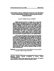
5 For each n ∈ {2, 3, . . .}, there is an one-to-one correspondence between the class Fn and the class H of all factor classes of positive distance functions related to the equivalence F ∼ G if and only if G(x) = F xc for some c > 0. In the following, we illustrate the construction method by few examples. Example 1. Let F be equal to a Dirac function1 focused at point x0 = 1,

0, x < 1, F (x) = δ1 (x) = 1, 1 ≤ x, then, as it is also shown in [8], by the Williamson n-transform we get generator 1 fn (x) = 1 − x n−1 of the weakest n-dimensional Archimedean copula, i.e., the −1 , see Figure 2. By rescaling non-strict Clayton copula with parameter λ = n−1 f (x) generator to fñ (x) = f (1/2) , x ∈ [0, 1], the copula would not change, yet such a generator is fixed to the value fñ 1 = 1, which we will use later to show 2

convergence. 1Dirac function is defined as δ (x) = x0

6

0,

x < x0 ,

1,

x ≥ x0 .


Figure 2. Dirac function F , the corresponding generators fn for different n and rescaled generators fñ .

Example 2. Let F be a uniform probability distribution function ⎧ ⎪ x < a, ⎨0, with 0 ≤ a < b, F (x) = x−a b−a , a ≤ x < b ⎪ ⎩ 1, b ≤ x. Then for dimension n = 2 we get

∞ x 2−1 (−1) 1− F (t)dt f2 (x) = t x ⎧ 1 b x ⎪ 1 − ⎪ t b−a dt, x < a, a ⎨ b 1 = dt, a ≤ x < b, 1 − xt b−a x ⎪ ⎪ ∞ ⎩ x 1 − t 0 dt, b ≤ x, x ⎧ b x log( a ) b 1 ⎪ ⎪ ⎨ b−a [t − x log t]a = 1 − b−a , =

1

⎪ b−a [t − ⎪ ⎩ 0,

b x log t]x

=

b b−a

−

b x+x log( x ) , b−a

x < a, a ≤ x < b, b≤x

(where F denotes a first derivative of F ) from which the corresponding generator can be obtained only numerically, and so is the case also with the higher dimensions, e.g., ⎧ b 2x log( a ) x2 ⎪ ⎪ x < a, ⎨1 − b−a + ab , b (−1) b x2 f3 (x) = b−a − 2x log x − (b−a)b , a ≤ x < b, ⎪ ⎪ ⎩ 0, b ≤ x, displayed in Figure 3. Setting a = 0 we get τ = 0 regardless of parameter b, which is in clear accordance with Theorem 5. 7


Figure 3. Uniform U(a,b) probability distribution function F and pseudoinverses of the corresponding generators fn .

We continue with the examples of constructing generators of non-strict Archimedean copulas while restricting the support of univariate distribution in the unit interval. By applying a suitable increasing transformation (such as power function) to a positive distance function on [0, 1] we obtain a new distribution. Example 3. Consider a positive distance function F (x) = min(1, x2 ) and the corresponding density F (x) = 2x on [0, 1]. Then

∞ x 2−1 (−1) 1− f2 (x) = dF (t) t x ⎧ 1 ⎪ ⎨ (t − x) 2t dt = (1 − x)2 , 0 ≤ x ≤ 1, t = x ⎪ ⎩0, 1 0. Observe that limx→0 F (x) = δ0 (x) while limx→∞ F (x) = δ1 (x). Then ⎧ xp −px+p−1 ⎪ , 0 ≤ x ≤ 1 ∧ p = 1, ⎨ p−1 (−1) f2 (x) = x(log x − 1) + 1, 0 ≤ x ≤ 1 ∧ p = 1, ⎪ ⎩ 0, 1 < x. 8


Figure 4. Illustration of Example 3 with non-invertible case n = 3.

Though it lacks an explicit inverse, the copulas that it generates cover almost 2p whole dependence range with τ = 1 − 1+p , τ ∈ (0, 1), and we will use it later to demonstrate approximation approach. Figure 5 shows simulations from this parametric copula family for p = 0.5 and p = 2. The only tail dependence is present at the upper tail for p ∈ (0, 1). It is interesting to illustrate also the inverse Williamson n-transform.

p = 0.5

p=2

Figure 5. Sampling from copula family constructed in Example 4.

Example 5. Let us take a generator of: • the Ali-Mikhail-Haq copula f (x) = x1 − 1 corresponding to the parameter λ = 1 and denote by Fn , n = 2, 3, . . . , a positive distance function related x n 1 x xn−1 to f through (6). Then Fn (x) = 1 − 1+x − (1+x) 2 − · · · − (1+x)n = 1+x which can be viewed as a parametric subfamily of all positive valued distribution functions Fp with any positive parameter p; 9


• the product copulaf (x) = − p1 log x with constantp > 0 and inverse f −1 (x) = exp(−px). From (6) for n = 2 we get F (x) = 1 − exp(−px)(1 − px). By comparing the density ∂F∂x(x) = p2 x exp(−px) and the convolution of two exponential distribution Dλ densities with parameter λ > 0,

x λ exp(−λt)λ exp −λ(x − t) dt = λ2 x exp(−λx) 0

it becomes clear that the resulting distribution is a distribution of the random variable Y = X1 +X2 , where X1 , X2 ∼ Dλ are independent (and identically distributed) random variables. The relation holds for any n ≥ 2, thus (6) yields a cumulative distribution function of the sum of i.i.d. random i−1 variables X1 , . . . , Xn ∼ Dp , FX1 +···+Xn (x) = 1 − exp(−px) ni=1 (px) (i−1)! with p > 0 which defines the Erlang distribution with rate parameter p and shape parameter n. To complete the examples, let us illustrate also the Laplace transform. Example 6. Starting with positive distance function of: • discrete random variable with probability mass concentrated in λ > 0, i.e., Dirac function F (x) = 0 for x < λ and 1 otherwise, then the Laplace transform leads through g(x) = exp(λx) to the product copula Π. • exponential distribution F (x) = 1 − exp(−λx), λ > 0, we get f −1 (x) = λ ( x+λ ) and f (x) = λ( x1 − 1) which generates the same copula (Clayton copula with parameter equal to 1) regardless of the choice of λ. Now we focus on the Dirac function since it can be viewed as a building block for distribution functions of a random variable with probability mass concentrated in l discrete points. Immediately a question arises: if such a distribution functions can approximate distribution of a continuous r.v. (for any l, going possibly to infinity), does this convergence imply also a convergence of the corresponding generators and even a convergence of the generated copulas?

3. Convergence theorems

1

Let (Fm )m be a sequence of distribution functions and let F be a distribution function. We say that the sequence of distribution functions Fm , m = 1, 2, . . . , weakly converge to distribution function F if lim Fm (x) = F (x)

m→∞

holds for any point x ∈ R in which F is continuous. The weak convergence will be w denoted by Fm → F . 10


er continuity theorem [14] ensures the convergence ∞ ∞Recall that the Lévy-Cram´ h(t)dFm (t) −→ −∞ h(t)dF (t), where h : ]− ∞, ∞[ → ]− ∞, ∞[ is a contin−∞ m→∞

uous bounded real function and Fmw→F . Obviously, for any n ≥ 2 and x < 0, n−1 the function h : ] − ∞, ∞[→] − ∞, ∞[ given by h(t) = 1 + xt δ−x (t) is continuous and bounded. This fact proves the next important result.

6

Let a sequence (Fm )m of distance functions converge weakly to w a distance function F , Fm → F . Then, for any n ≥ 2, the corresponding additive generators f , fm , m = 1, 2, . . . , of n-dimensional Archimedean copulas are related by the pointwise convergence fm −→ f . m→∞

P r o o f. Based on the Williamson n-transform (7) and the Lévy-Cramér continuity theorem, gm → g pointwisely, and all functions g, gm , m = 1, 2, . . . are convex, continuous and strictly increasing. Then also the related additive generators f , fm , m = 1, 2, . . . , satisfy fm → f pointwisely. The reverse of Theorem 6 is based on the next lemma.

1 Let (fm )m , f be convex real functions defined on a real interval ]α, β[ such that fm → f pointwisely. Then for any point a ∈]α, β[, where f (a) exists it holds limm→∞ f (a− ) = f (a) = limm→∞ fm (a+ ). P r o o f. Note that due to the convexity, the left derivatives fm (a− ), fm (a− ) + + and the right derivatives fm (a ), fm (a ) exist at each point a ∈]α, β[. More over, the convexity ensures also that fm (x) ≥ fm (a) + (x − a)fm (a− ) and + fm (x) ≥ fm (a) + (x − a)fm (a ) for any m = 1, 2, . . . and x ∈]α, β[. Fix m (a) (a− ) ≤ fm (x)−f and thus lim sup fm (a− ) ≤ a ∈]α, β[. Then, for any x > a, fm x−a f (x)−f (a) (a) . Therefore lim sup fm (a− ) ≤ limx→a+ f (x)−f = f (a+ ). Similarly, x−a x−a − (a− ) ≥ f (a− ), which implies the existence of the limit of fm (a ) m , lim inf fm (a− ) = f (a) if f (a) exists. whenever f (a− ) = f (a+ ) = f (a), limm→∞ fm Using similar arguments, if f (a) exists, then also limm→∞ fm (a+ ) = f (a).

Based on Lemma 1, the next result follows directly.

7 Let fm , f ∈ Fn, m = 1, 2, . . . , be additive generators of n-dimensional Archimedean copulas, such that fn → f pointwisely on ]0, 1]. Let Fm , F , m = 1, 2, . . . , be the related distance function obtained by means of the transw form (6). Then Fm → F . (k)

P r o o f. Based on Theorem 2, gm , m = 1, 2, . . . , and g (k) are convex functions for k = 0, 1, . . . , n − 2. The pointwise convergence fm → f on ]0, 1] implies the pointwise convergence gm → g on ]−∞, 0[, and due to Lemma 1, repeated (n−2)(n−2) -times, it holds limm→∞ gm (x) = g (x), . . . , limm→∞ gm (x) = g (n−2) (x) and 11

´S ˇ BACIGAL ´ — MARIA ´ ˇ ÍMALOVA ´ TOMA ZD (n−1)

limm→∞ gm (x− ) = g (n−1) (x) at each point x ∈] − ∞, 0[, where g (n−1) (x) exists. Therefore, limm→∞ Fm (x) = F (x) at each point x ∈]0, ∞[, where the function g (n−1) (x− ) is continuous, i.e., where F (x) is continuous. Thus Fmw→F. The next result from [10] was shown for (n-ary) continuous Archimedean triangular norms (however, any (n-ary) Archimedean copula is also a continuous Archimedean t-norm) and later for Archimedean copulas in [3, Proposition 2].

8

Let C, Cm : [0, 1]n → [0, 1], m = 1, 2, . . . , be continuous Archimedean copulas, generated by additive generators f, fm: [0, 1] → [0, ∞], m = 1, 2, . . . , respectively. Then the following are equivalent. i) Cm −→ C pointwisely. m→∞

ii) There are positive constants cm , m = 1, 2, . . . , so that cm fm → f pointwisely. Combining Theorems 6, 7, 8 we have the next result which can be exploited when approximating Archimedean copulas.

2 The following convergences of related objects are equivalent (for any n ≥ 2) : w

i) for distance functions, Fm → F ; ii) for additive generators from Fn , fm → f pointwisely on ]0, 1]; iii) for n-dimensional Archimedean copulas, Cm → C pointwisely. Recall that each distance function F can be obtained as a weak limit of (bounded) discrete distance functions Fm , and that each bounded discrete distance function is, in fact, a convex combination of Dirac distance functions.

4. Approximation In this section we are interested mainly in (n = 2)-dimensional case, since it is of most benefit in practice. Therefore hereafter the subscript with generator f gains a different meaning: the number of pieces f is approximated by. Example 7. Let F (x) = min(1, x2 ) be the positive distance function from the Example 3 and function ⎧ 1 ⎪ ⎨0, x < 2 , 1 1 δ1 (x) = 14 , 12 ≤ x < 1, F2 (x) = F δ 12 (x) + F (1) − F ⎪ 2 2 ⎩ 1, 1 ≤ x 12


approximates F by means of a3 sum of m = 2 Dirac functions concentrated 1 1 in respective points 2 , 4 , 1, 4 . Then the Williamson transform with n = 2 yields ⎧ 5 1 ⎪ ⎨1 − 4 x, x < 2 , x x 1 3 (−1) 3 3 1 = 4 − 4 x, 2 ≤ x < 1, f2 (x) = max 0, 1 − 1 + max 0, 1 − ⎪ 4 4 1 ⎩ 2 0, 1 ≤ x. From Example 7 illustrated in Figure 6 we see that for n = 2 the additive (−1) is piecewise linear and does not coincide with f (−1) in generator inverse f2 the interval ]0, 1[.

Figure 6. Approximation by the sum of m = 2 Dirac functions.

Dividing an interval [a0 , am ] by points {ai }i=1,...m , a0 < a1 < · · · am , with concentration of probability given by some probability mass function p(x), the approximate positive distance function Fm (x) =

m

p(ai )δai (x)

i=1

is then transformed by (7) to the generator inverse (related to some n-dimensional Archimedean copula) n−1 n−1 m x x (−1) p(ai ) 1 − = p(ai ) max 0, 1 − . (9) fm (x) = ai ai x