Proceedings of the European Control Conference 2007 Kos, Greece, July 2-5, 2007
WeA04.5
Convergence of Q-learning with linear function approximation Francisco S. Melo Institute for Systems and Robotics, Instituto Superior Técnico, Lisboa, PORTUGAL
M. Isabel Ribeiro Institute for Systems and Robotics, Instituto Superior Técnico, Lisboa, PORTUGAL
[email protected]
[email protected]
Abstract— In this paper, we analyze the convergence properties of Q-learning using linear function approximation. This algorithm can be seen as an extension to stochastic control settings of TD-learning using linear function approximation, as described in [1]. We derive a set of conditions that implies the convergence of this approximation method with probability 1, when a fixed learning policy is used. We provide an interpretation of the obtained approximation as a fixed point of a Bellman-like operator. We then discuss the relation of our result with several related works as well as its general applicability.
I. INTRODUCTION Reinforcement learning addresses the problem of an agent faced with a sequential decision problem and using evaluative feedback as a performance measure [2]. Reinforcement learning methods compute a mapping from the set of states of the agent to the set of possible actions. Such mapping is called a policy and it is customary to define a utility-function, or value-function, estimating the practical utility of each particular policy. Value-based methods such as TD-learning [3], Q-learning [4] or SARSA [5] have been exhaustively covered in the literature and, under mild assumptions, have been proven to converge to the desired solution [6]–[8]. However, many such algorithms require explicit representation of the state-space, and is often the case that the state-space is unsuited for explicit representation. Instead, the decision-maker should be able to generalize its action-pattern from the collected experience. Gerald Tesauro’s backgammon player [9], [10], which was able to learn master-level play, boosted the interest in the topic of generalization. In his work, Tesauro combines temporal-difference learning with neural networks, and the impressive results of his learning agent have established the applicability of function approximation in reinforcement learning problems. Other works on generalization include [11]–[14]. In this paper, we describe Q-learning with linear function approximation. This algorithm can be seen as an extension to control problems of temporal-difference learning using linear function approximation as described in [1]. Convergence of Q-learning with function approximation has been a long standing question in reinforcement learning. Our result provides a contribution towards the solution of this problem. We identify a set of conditions that ensure convergence of this method with probability 1. We also provide an interpretation for the obtained approximation as the fixed-point of a Bellman-like operator. Finally, we
ISBN: 978-960-89028-5-5
discuss our convergence results in face of those reported using so different approaches as soft-state aggregation [13] or interpolation-based Q-learning [14]. In the next section, we describe the framework addressed throughout this paper. We then present the algorithm and the main result of the paper, concerning its convergence. We conclude the paper with some discussion. Details of the proof are found in the appendix. II. THE MARKOV DECISION PROCESS FRAMEWORK Let X be a compact subspace of Rp and {Xt } a X -valued controlled Markov chain. The transition probabilities for the chain are given by a probability kernel P [Xt+1 ∈ U | Xt = x, At = a] = Pa (x, U ), where U ⊂ X . The A-valued process {At } represents the control process; At is the control action at time instant t and A is the finite set of possible actions. The agent aims at choosing the control process {At } so as to maximize the infinite-horizon total discounted reward, i.e., # "∞ X t γ R(Xt , At ) | X0 = x , V ({At } , x) = E t=0
where 0 ≤ γ < 1 is a discount-factor and R(x, a) represents a random “reward” received for taking action a ∈ A in state x ∈ X. We assume throughout this paper that there is a deterministic function r : X × A × X −→ R assigning a reward r(x, a, y) every time a transition from x to y occurs after taking action a and that Z r(x, a, y)Pa (x, dy). E [R(x, a)] = X
This simplifies the notation without introducing a great loss in generality. We further assume that there is a constant R ∈ R such that |r(x, a, y)| < R for all x, y ∈ X and all a ∈ A.1 We refer to the 5-tuple (X , A, P, r, γ) as a Markov decision process (MDP). Given the MDP (X , A, P, r, γ), the optimal value function V ∗ is defined for each state x ∈ X as # "∞ X t ∗ γ R(Xt , At ) | X0 = x V (x) = max E {At }
1 This
t=0
assumption is tantamount to the standard requirement that the rewards R(x, a) have uniformly bounded variance.
2671
WeA04.5 to be made clear. By defining a suitable recursion for θ, we reduce the determination of the infinite-dimensional function Q∗ to the determination of a finite-dimensional vector θ∗ .
and verifies V ∗ (x) = max a∈A
Z
X
£ ¤ r(x, a, y) + γV ∗ (y) Pa (x, dy),
which is a form of the Bellman optimality equation. From the optimal value function, the optimal Q-values Q∗ (x, a) are defined for each state-action pair (x, a) ∈ X × A as Z £ ¤ ∗ Q (x, a) = r(x, a, y) + γV ∗ (y) Pa (x, dy). (1) X
From the optimal Q-function Q∗ it is possible to define a mapping δ ∗ : X −→ A as δ ∗ (x) = arg max Q∗ (x, a), a∈A
for all x ∈ X and the control process {At } defined by At = δ ∗ (Xt ) is optimal in the sense that V ({At } , x) = V ∗ (x), for all x ∈ X . The mapping δ ∗ is an optimal policy for the MDP (X , A, P, r, γ). More generally, we define a (stochastic) policy as a mapping δ : X ×A −→ [0, 1] that generates a control process {At } verifying P [At = a | Xt = x] = δ(x, a), for all t. Simply stated, δ(x, a) defines the probability of choosing each action a in state x. Clearly, sincePδ(x, ·) is a probability distribution over A, it must satisfy a∈A δ(x, a) = 1, for all x ∈ X . In the particular case where, for every x ∈ A, δ(x, a) = 1 for some a ∈ A, we say that δ is a deterministic policy and simply denote by δ(x) the action chosen at state x with probability 1. In this case, a control process is generated by policy δ if At = δ(Xt ) for all t. We write V δ (x) instead of V ({At } , x) if the control process {At } is generated by a policy δ. The optimal control process can be obtained from the optimal policy δ ∗ , which can in turn be obtained from Q∗ . Therefore, the optimal control problem is solved once the function Q∗ is known for all pairs (x, a) ∈ X × A. The original Q-learning algorithm [4] uses a stochastic iterative update to determine the optimal Q-values. The update-rule for Q-learning is £ Qk+1 (x, a) = Qk (x, a) + αk R(x, a)+ ¤ (2) + γ max Qk (X(x, a), b) − Qk (x, a) , b∈A
where Qk (x, a) is the k th estimate of Q∗ (x, a), X(x, a) is a X -valued random variable obtained according to the probabilities definedPby Pa and αk are step-sizes verifying P 2 k αk = ∞ and k αk < ∞. Notice that R(x, a) and X(x, a) can be obtained through some simulation device, not requiring the knowledge of either P or r. Q-leaning was originally proposed to deal with MDPs with finite state-spaces. When X is an infinite set, it is not possible to straightforwardly apply the update rule (2), since it explicitly updates the Q-value for each individual stateaction pair and there are infinitely many such pairs. In this paper we consider a parameterized family Q of functions Qθ : X ×A −→ R, where θ is a parameter in RM . We want to determine the point θ∗ in parameter space such that Qθ∗ is the best approximation of Q∗ in Q, in a sense yet
III. MAIN RESULT In this section, we establish the convergence properties of Q-learning when using linear function approximation. As will be seen, the result derived herein can be seen as a generalization of other results from the literature (such as those reported on methods based on discretization [15], softdiscretization [13] or interpolation [14]). We consider a family of functions Q = {Qθ } parameterized by a finite-dimensional parameter vector θ ∈ RM . We admit the family Q to be linear in that if q1 , q2 ∈ Q, then so does αq1 +q2 for any α ∈ R. Q is therefore the linear span of a set of M linearly independent functions ξi : X × A −→ R, and each q ∈ Q can be written as q(x, a) =
M X
ξi (x, a)θ(i),
i=1
for all pairs (x, a) ∈ X ×A, where θ(i) is the ith component of the vector θ ∈ RM . Given now a set {ξi , i = 1, . . . , M } of linearly independent functions and a vector θ ∈ RM , we denote interchangeably by Qθ and Q(θ) the function Qθ (x, a) =
M X
ξi (x, a)θ(i) = ξ ⊤ (x, a)θ,
(3)
i=1
where ξ(x, a) is a vector in RM with ith component given by ξi (x, a) and the superscript ⊤ represents the transpose operator. Let δ be a stochastic stationary policy and suppose that {xt }, {at } and {rt } are sampled trajectories obtained from the MDP (X , A, P, r, γ) using policy δ. In the original Qlearning algorithm, the Q-values are updated according to (2), using the temporal difference at time t, ∆t = rt + γ max Qt (xt+1 , b) − Qt (xt , at ). b∈A
The temporal difference ∆t works as a 1-step estimation error with respect to the optimal function Q∗ ; the update rule in Q-learning “moves” the estimates Qt closer to the desired function Q∗ , minimizing the expected value of ∆t . Applying the same underlying idea, we obtain the following update rule for the vector θt : ¡ θt+1 = θt + αt ∇θ Qθ (xt , at ) rt + ¢ + γ max Qθt (xt+1 , b) − Qθt (xt , at ) = b∈A ¡ = θt + αt ξ(xt , at ) rt + ¢ (4) + γ max Qθt (xt+1 , b) − Qθt (xt , at ) . b∈A
Notice that (4) updates θt using the temporal difference ∆t as the error. The gradient ∇θ Qθ provides the “direction” in which this update is performed. Roughly speaking, (4) can be seen as a gradient descent update using αt ∆t as the step-size,
2672
WeA04.5 and (4) iteratively determines the parameter θ corresponding to the function in Q minimizing the expected value of ∆t .2 We show that, under some regularity assumptions on the Markov chain (X , Pδ ) obtained using the policy δ, the trajectories of the algorithm closely follow those of an associated ODE with a globally asymptotically stable equilibrium point θ∗ . Therefore, the sequence {θt } defined recursively by (4) will converge w.p.1 to the equilibrium point θ∗ of the ODE. We also show that this equilibrium point is the fixed-point of a Bellman-like operator, θ∗ = PHQ(θ∗ ),
(5)
where P represents a projection and H is the Bellman operator (Hq)(x, a) =
Z
X
ˆ
˜ r(x, a, y) + γ max q(y, b) Pa (x, dy). b∈A
(6)
We now state our main convergence result. Given a MDP (X , A, P, r, γ), let δ be a stationary stochastic policy and (X , Pδ ) the corresponding Markov chain with invariant probability measure µX . Denote by Eµδ [·] the expectation w.r.t. the probability measure µδ defined for every set Z × U ⊂ X × A as Z X δ(x, a)µX (x). µδ (Z × U ) = Z a∈U
Theorem 3.1: Let (X , A, P, r, γ) be a Markov decision process and assume the Markov chain (X , Pδ ) to be geometrically ergodic with invariant probability measure µX . Suppose that δ(x, a) > 0 for all a ∈ A and µX -almost all x ∈ X. Let Ξ = {ξi , i = 1, . . . , M } be a set of M bounded, linearly independent functions defined X × A and taking Pon N values in R. In particular, admit that i=1 |ξi (x, a)| ≤ 1 for all (x, a) ∈ X × A. Then, the following hold. 1) Convergence For any initial condition θ0 ∈ RM , the algorithm ¡ θt+1 = θt + αt ξ(xt , at ) rt + ¢ (7) + γ max Qθt (xt+1 , b) − Qθt (xt , at ) b∈A
converges w.p.1 as long as the step-size sequence {αt } verifies X X αt = ∞ αt2 ≤ ∞. t
t
2) Limit of convergence Under these conditions, the limit θ∗ of (7) verifies Qθ∗ (x, a) = (PQ HQθ∗ )(x, a),
and the matrix Σ is given by £ ¤ Σ = Eµδ ξ(x, a)ξ ⊤ (x, a) . Proof: See Appendix I. To convey a deeper insight on the conditions of the Theorem, we remark that the geometric ergodicity assumption and the requirement that δ(x, a) > 0 for all a ∈ A and µX -almost all x ∈ X can be interpreted as a continuous counterpart to the usual condition that all state-action pairs are visited infinitely often. In fact, geometric ergodicity implies that all the regions of the state space with positive µX measure are “sufficiently” visited [17], and the condition that δ(x, a) > 0 ensures that, at each state, every action is “sufficiently” tried. On the other hand, geometric ergodicity guarantees that the Markov chain (X , Pδ ) obtained using the learning policy δ converges exponentially fast to stationarity, and thus the analysis of convergence of the algorithm can be done in terms of a “stationary version” of it.3 We also notice that the requirements on the basis functions ξi simply guarantee (in a rather conservative way) that no two functions ξi lead to “colliding updates”, as in the known counter-example in [16]. IV. RELATED WORK In [1], Tsitsiklis and Van Roy provide a detailed analysis of temporal difference methods. In the referred work, the authors establish important results regarding the convergence/divergence of such methods when linear function approximation is used: the trajectories of TD-learning closely follow those of an associated globally asymptotically stable ODE and thus converge to the unique equilibrium point of such ODE. They also provide error bounds for the obtained approximation and an interpretation of the limit function as the fixed point of a composite operator PV T(λ) , where PV is an orthogonal projection into a linear function space V and T(λ) is a TD operator. The authors remark, however, that if off-policy updates are used (such as those in Qlearning) their convergence results no longer hold. More detailed analysis of this method as well as some variations can be found in [6], [12], [18]. Least-squares temporal difference learning methods (LSTD) depart from the same idea and propose an alternative method to estimate the same approximation used in TDlearning with function approximation [19]. As established by Tsitsiklis and Van Roy [1], TD-learning with linear function approximation converges in the limit to a parameter vector θ∗ that verifies a linear system of the type Aθ∗ + b = 0,
(8)
where PQ denotes the orthogonal projection operator on Q defined by (PQ Q)(x, a) = ξ ⊤ (x, a)Σ−1 Eµδ [ξ(z, u)Q(z, u)] . 2 We remark that this interpretation lacks rigor and aims only at clarifying the underlying working of the algorithm. We refer to [16], where reinforcement learning is addressed using gradient methods.
where the matrices A and b arise from a “stationary version” of the algorithm. LSTD estimates directly the matrices A and b from the sample trajectories of the underlying Markov chain, thus converging to the same limiting approximation 3 In particular, exponential convergence to stationarity ensures that the analysis of the trajectories of the sequence {θt } can be performed in terms of the trajectories of an associated ODE.
2673
WeA04.5 and with some extra argued advantages [19]. Although not exactly in the line of the algorithm described herein, it is important to mention LSTD as closely related with TDlearning with function approximation. Szepesvári and Smart [14] extend the results in [1] to control settings. In this paper, the authors propose a modified version of Q-learning that approximates the optimal Qvalues of a given set of sample points and then uses interpolation to approximate Q∗ at any query point. The update rule for interpolation-based Q-learning uses a spreading function similar to the one used in multi-state Q-learning [20]. As in [1], the authors establish convergence w.p.1 of the algorithm and provide an interpretation of the limit point as the fixedpoint of a composite operator PH, where P is a projectionlike operator and H can be interpreted as a modified TDlearning operator. Interpolated Q-learning approximates the value of the optimal Q-function at a previously chosen set of sample points. Closely related with the method in [14] is the soft-state aggregation algorithm by [13]. In this work, the authors propose the use of a “soft”-partition of the state-space: the state-space is split into “soft” regions (each state x belongs to region i with a probability pi (x)) and an “average” Q-value Q(i, a) is defined for each region-action pair. Each of these regions is then treated as a “hyper-state” and the method uses standard Q-learning updates to determine the average Qvalues for each region. The function Q∗ is then P approximated for a state-action pair (x, a) as Q∗ (x, a) ≈ i pi (x)Q(i, a). Both interpolated Q-learning and Q-learning with softstate aggregation provide important positive convergence results for Q-learning using function approximation, arising as encouraging counterparts to the divergent counterexamples reported in several works [1], [16]. Finally, Atkeson et al. [21] describe the application of local weighted regression methods to estimate the model (namely the kernel P and the reward function r) in a continuousstate reinforcement learning problem and this fundamental idea is generalized in [22]. In the latter work, the authors establish convergence in probability and derive the limiting distribution of the obtained approximation. The authors also address the bias-variance tradeoff in reinforcement learning problems. In the next section we conclude the paper by further discussing our results in face of some of the aforementioned works.
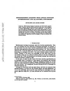
Goal
Fig. 1. Simple indoor environment.
The navigation problem can be described by a MDP (X , A, P, r, γ), where • X = [0; 1] × [0; 1]; • A = {N, S, E, W }; • Each action in A moves the robot in the corresponding direction a random distance between 0 and 0.3; • The reward function r assigns a reward of +10 for every transition triplet (x, a, y) such that ky − (1; 1)k < 0.1 and 0 otherwise. When the robot reaches the goal region, its position is randomly reset to any point in the room, independently of the agent’s action. We applied Q-learning with function approximation to this MDP using three different sets of basis functions. The first set of basis functions was obtained by dividing the statespace into a uniform grid of 0.1×0.1 rectangles. The second set was obtained by scaling the four linear surfaces σi , i = 1, . . . , 4, defined at each point (x, y) as σ1 ((x, y)) = x; σ3 ((x, y)) = y;
σ2 ((x, y)) = 1 − x; σ4 ((x, y)) = 1 − y.
Finally, the last set of functions considered 4 normalized gaussian kernels centered around each of the 4 corners of the rectangle [0; 1]×[0; 1]. All basis functions further considered an action-dependent component, allowing the robot to learn different values for each function.5 TABLE I C OMPARATIVE RESULTS FOR Q- LEARNING WITH FUNCTION APPROXIMATION FOR THE DIFFERENT SETS OF BASIS FUNCTIONS .
WE
PRESENT THE AVERAGE TOTAL DISCOUNTED REWARD AND STANDARD DEVIATION OBTAINED OVER
Method
V. AN ILLUSTRATIVE EXAMPLE
Grid-based Plane-based Kernel-based
2′ 000 M ONTE -C ARLO RUNS . Q-learning
8.474 8.221 8.554
± ± ±
1.728 1.751 1.687
Consider the indoor environment depicted in Figure 1. A mobile robot is intended to navigate to the goal region, signaled with the dashed lines. The environment is a 1 × 1 square, and the state of the robot at each time instant is a pair (x, y) of coordinates.4 The coordinates of the goal corner are (1, 1).
For each set of basis functions, the agent was allowed to explore and learn during 20′ 000 time steps, and the obtained policy was then evaluated for 100 time steps. To test the
4 We use boldface symbols x and y to denote the physical coordinates of the robot to distinguish from the symbols x and y used to denote generic elements of the state-space X .
5 In other words, each state-dependent function f (x) led to |A| different basis functions ξia , where ξia (x, u) = f (x)Ia (u) for every (x, u) ∈ X × A.
2674
WeA04.5 obtained policy we ran 2′ 000 Monte Carlo independent trials. The results are presented in Table I, corresponding to the mean and standard deviation of the obtained discounted reward with the learnt policy. Notice that all approximations lead to a similar performance. This means that all sets of basis functions provided an equally accurate approximation. Figure 2 depicts the policies learnt using each approximation. We present in Figure 3 a detail of the policy obtained using Q-learning with a plane-based approximation. This detail helps to clarify the different patterns observed in the policy representations of Figure 2. Notice that all policy representations correspond to similar behavior, which is moving to the upper right corner (as expected). Optimal policy for Q−learning 1
0.98
y
0.96
0.94
0.92
0.9 0.9
0.92
0.94
0.96
0.98
1
1.02
x
Fig. 3. Detail of Figure 2 a).
To further illustrate the similarity of the learned functions for all sets of basis functions, we present in Figure 4 a representation of the obtained value functions for each of the different sets of basis functions. VI. CONCLUDING REMARKS From all the works described in Section IV, the approach in [1] is the closest to the one presented here. In [1], the authors make use of the operator T(λ) that is a contraction in the 2-norm. In this norm, the orthogonal projection PV is naturally defined and no additional conditions are required to ensure that PV is non-expansive. In this paper, we extend this approach to control settings. To this end, we are interested in approximating the fixed point of the operator H defined in (6). This operator is a contraction in the maximum norm and no orthogonal projection is naturally defined in a space with such a norm. However, by requiring that N X
|ξi (x, a)| ≤ 1
(9)
i=1
for all (x, a), we guarantee that the operator H is also a contraction in θ, which implies the exponential stability of the associated ODE. Another interesting remark is that (9) implies that the functions {ξi , i = 1, . . . , M } can be used to define a softpartition of X . This means that the method presented here can be cast as a modified version of Q-learning with softstate aggregation. Or, in yet another point-of-view, convergence of Q-learning with soft-state aggregation arises as a consequence of our convergence results.
It is important to emphasize that the condition (9) is not too restrictive. In fact, given a set of linearly independent functions Ξ = {ξi , i = 1, . . . , M }, we can easily ensure such bound by scaling the functions in Ξ. We further emphasize that the condition (9) is trivially verified in many common approximation strategies. For example, approximation strategies based on state-space discretization [15] or convex interpolation approximators [14] verify the bound in (9), as do soft-discretization architectures [13]. We finish with four concluding remarks. First of all, the conditions of Theorem 3.1 on the Markov chain are similar to those required in [1] and in [14]. This places those works as well as this paper in a common line of work and, basically, leading to concordant conclusions. We also notice that, although the conditions of Theorem 3.1 are posed as sufficient (and not necessary), the nonverification of some of the conditions may lead to divergence. As a simple illustration, in the example of divergence presented in [16], the functions used in the linear approximation scheme arenot linearly independent and do not verify the bound in (9). Another observation is related with the rate of convergence of the algorithm presented herein. Our proof of convergence uses standard results from stochastic approximation algorithms and several known results exist describing the rates of convergence for this class of methods. These results [23] lead to the interesting conclusion that the rate of convergence of our algorithm (which works on infinite state-spaces) is essentially similar to that of standard Q-learning as described in [24] (which works on finite state-spaces). Finally, the method proposed herein is off-policy, i.e., learns the value of the optimal policy while executing a different policy during learning. Also, unlike the approach in [1], we make no use of eligibility traces, which could improve the overall performance of the algorithm (the use of eligibility traces guarantees tighter error bounds). Nevertheless, there is no formal reason why the algorithm in this paper cannot be modified so as to accommodate eligibility traces. Furthermore, the convergence result presented can be of use in the analysis of an on-policy version of the algorithm, by using results on the stability of perturbed ODEs. A PPENDIX I PROOF OF THEOREM 3.1 We separately establish each of the three statements in Theorem 3.1. To prove the Statement 1, we write (7) in the form θt+1 = θt + αt+1 H(θt , Yt+1 ), and use Theorem 17 of [25]: we show that the associated ODE has a globally asymptotically stable equilibrium point, which implies the existence of a Lyapunov function U verifying the requirements of the referred theorem. That establishes convergence of (7) w.p.1. To prove Statement 2 of Theorem 3.1, we provide an interpretation of the equilibrium point of the ODE associated with algorithm (7) as the fixed point of a composite operator.
2675
WeA04.5
Optimal policy for Q−learning 1
0.9
0.9
0.8
0.8
0.7
0.7
0.6
0.6
0.5
0.5
y
y
Optimal policy for Q−learning 1
0.4
0.4
0.3
0.3
0.2
0.2
0.1
0.1
0
0
0.1
0.2
0.3
0.4
0.5 x
0.6
0.7
0.8
0.9
0
1
0
0.1
a) Grid-based approximation;
0.2
0.3
0.4
0.5 x
0.6
0.7
0.8
0.9
1
b) Linear-based approximation; Optimal policy for Q−learning
1 0.9 0.8 0.7
y
0.6 0.5 0.4 0.3 0.2 0.1 0
0
0.1
0.2
0.3
0.4
0.5 x
0.6
0.7
0.8
0.9
1
c) Kernel-based approximation. Fig. 2. Policy learnt by Q-learning with function approximation.
Value surface for Q−learning
Value surface for Q−learning
12
25
10
20
V(x,y)
V(x,y)
8 6 4
15 10 5
2 0 1
0 1 1
1
0.8
0.5
0.8
0.5
0.6
0.6
0.4 y
0
0.4
0.2 0
0
y
x
a) Grid-based approximation;
0.2 0
x
b) Linear-based approximation; Value surface for Q−learning
20
V(x,y)
15
10
5
0 1 1 0.8
0.5
0.6 0.4
y
0
0.2 0
x
c) Kernel-based approximation. Fig. 4. Representation of the optimal value-function learnt by Q-learning with function approximation.
2676
WeA04.5 Explicit calculations now yield
A. Convergence of the iterates We start by writing (7) as
X d 1−p kθt − θ∗ kp = kθt − θ∗ kp (θt (i) − θ∗ (i))p−1 · dt i
θt+1 = θt + αt+1 H(θt , Yt+1 ), where Yt+1 = (Xt , At , Xt+1 ). Since the chain {Xt } is geometrically ergodic and δ(x, a) > 0 for µX -almost all x ∈ X , it follows that so is the chain {Yt }. Let µ ˆ be the corresponding invariant probability measure. On the other hand, since X is compact and A is finite, {Yt } also lies in a compact set. Finally, since the functions ξi are clearly bounded and so are the rewards r(x, a, y), H verifies the bound kH(θ, Y )k∞ ≤ C(1 + kθk∞ ) for some C > 0. Finally, the geometric ergodicity of {Yt } and the fact that δ does not depend on θ ensure that the requirements of Theorem 17 of [25] can be applied, and convergence of {θt } w.p.1 is established as long as the ODE θ˙t = h(θt ),
(10)
with h ¡ h(θ) = Eµˆ ξ(x, a) r(x, a, z)+
¢i + γ max ξ ⊤ (z, b)θ − ξ ⊤ (x, a)θ ,
(11)
· (h1 (θ)i − h1 (θ∗ )i )− X 1−p − kθt − θ∗ kp (θt (i) − θ∗ (i))p−1 · i
· (h2 (θ)i − h2 (θ∗ )i ),
where we denoted by h1 (θ)i the ith component of h1 (θ) and similarly for h2 . Applying Hölder’s inequality to the summations leads to d kθt − θ∗ kp ≤ kh1 (θ) − h1 (θ∗ )kp − kh2 (θ) − h2 (θ∗ )kp . dt
Taking the limit as p → ∞ and using (13) and (14) leads to d kθt − θ∗ k∞ ≤ γ kθt − θ∗ k∞ − kθt − θ∗ k∞ dt which, in turn, leads to d kθt − θ∗ k∞ ≤ (γ − 1) kθt − θ∗ k∞ . (15) dt Let λ = 1 − γ > 0. Upon integration, (15) becomes kθt − θ∗ k∞ ≤ e−λt kθ0 − θ∗ k∞ ,
b∈A
has a globally asymptotically stable equilibrium θ∗ . Proposition 1.1: The ODE θ˙t = h(θt ),
(12)
where h is defined in (11), has a globally asymptotically stable equilibrium θ∗ verifying the recursive relation θ∗ = PHQ(θ∗ ).
which in turn leads to ¸ · ¡ ¢ θ∗ = Σ−1 Eµˆ ξ(x, a) r(x, a, z) + γ max ξ ⊤ (z, b)θ
R EMARK : The operator H is defined in (6) and the projection operator P is defined for any real function q defined on X × A as Pq = Σ
−1
b∈A
and the proof is complete.
Eµˆ [ξ(x, a)q(x, a)] .
The fact that the equilibrium point θ∗ is globally asymptotically stable is sufficient to ensure the existence of a function U verifying the conditions of Theorem 17 in [25],6 which in turn establishes the convergence of the sequence {θt } w.p.1.
Proof: We start by rewriting h as h(θ) = h1 (θ) + h2 (θ), with
B. Limit of convergence
¸ · ¡ ¢ h1 (θ) = Eµˆ ξ(x, a) r(x, a, z) + γ max ξ ⊤ (z, b)θ
We have established that the sequence {θt } generated by (7) converges w.p.1. The limit point θ∗ is the globally asymptotically stable equilibrium of the ODE (12), verifying the following recursive relation:
b∈A
and
which establishes the existence of a globally asymptotically stable equilibrium point for (12). It is now clear that h(θ∗ ) = 0 is equivalent to ¸ · ¡ ¢ Eµˆ ξ(x, a) r(x, a, z) + γ max ξ ⊤ (z, b)θ = b∈A £ ¤ ⊤ = Eµˆ ξ(x, a)ξ (x, a)θ
£ ¤ h2 (θ) = Eµˆ ξ(x, a)ξ ⊤ (x, a)θ .
Some simple calculations lead to the conclusion that
θ∗ = PHQ(θ∗ )
kh1 (θ1 ) − h1 (θ2 )k∞ ≤ γ kθ1 − θ2 k∞
(13)
kh2 (θ1 ) − h2 (θ2 )k∞ ≤ kθ1 − θ2 k∞ .
(14)
or, more explicitly,
and On the other hand, any equilibrium point θ∗ of (12) must verify h(θ∗ ) = 0 or, which is the same,
θ∗ = Σ−1 EY [ξ(x, a)(HQθ∗ )(x, a)] , where Q(θ) is the function
h(θ) = h(θ) − h(θ∗ ).
Qθ (x, a) = ξ ⊤ (x, a)θ. 6 This
2677
guarantee arises from standard converse Lyapunov theorems.
(16)
WeA04.5 The purpose of (7) is to approximate the optimal Qfunction Q∗ by an element of the linear space Q spanned by the basis functions ξi ∈ Ξ. We would like to determine the element q ∗ ∈ Q that, in some sense, “best approximates” Q∗ . One possibility is to consider the orthogonal projection of Q∗ on Q. Denote the orthogonal projection operator on Q by PQ . Finding the projection of Q∗ on Q translates into finding the function f ∈ Q verifying f (x, a) = (PQ Q∗ )(x, a) = (PQ HQ∗ )(x, a). However, f thus defined is not a fixed point of any of the involved operators, and there is not an obvious procedure to write a stochastic approximation algorithm to find f . Therefore, we consider the function g verifying g(x, a) = (PQ Hg)(x, a).
(17)
The function g is a fixed point of the operator PQ H and can easily be implemented using stochastic approximation. It turns out that the projection PQ can be expressed as (PQ f )(x, a) = ξ ⊤ (x, a)Σ−1 EY [ξ(z, u)f (z, u)] for any function f . But this means that, given the limit point θ∗ of algorithm (7), the corresponding function Qθ∗ verifies Qθ∗ (x, a) = ξ ⊤ (x, a)(PHQθ∗ ) = = ξ ⊤ (x, a)Σ−1 EY [ξ(z, u)HQθ∗ (z, u)] = = (PQ HQθ )(x, a) where the second equality comes from (16). Finally, this implies that Qθ∗ verifies the fixed point equation in (17), which establishes statement (8) of Theorem 3.1. This concludes the proof of Theorem 3.1. ACKNOWLEDGEMENTS The authors would like to acknowledge the helpful discussions with João Xavier, from ISR/IST and the comments from the anonymous reviewers. This work was partially supported by the POS_C financing program, that includes FEDER funds. The first author acknowledges the PhD grant SFRH/BD/3074/2000.
[8] S. P. Singh, T. Jaakkola, M. Littman, and C. Szepesvari, “Convergence results for single-step on-policy reinforcement-learning algorithms,” Machine Learning, vol. 38, no. 3, pp. 287–310, 2000. [9] G. Tesauro, “TD-Gammon, a self-teaching backgammon program, achieves master-level play,” Neural Computation, vol. 6, no. 2, pp. 215–219, 1994. [10] ——, “Temporal difference learning and TD-Gammon,” Communications of the ACM, vol. 38, no. 3, pp. 58–68, 1995. [11] G. J. Gordon, “Stable function approximation in dynamic programming,” School of Computer Science, Carnegie Mellon University, Tech. Rep. CMU-CS-95-103, 1995. [12] B. Van Roy, “Learning and value function approximation in complex decision processes,” Ph.D. dissertation, Department of Electrical Engineering and Computer Science, Massachusetts Institute of Technology, June 1998. [13] S. P. Singh, T. Jaakkola, and M. I. Jordan, “Reinforcement learning with soft state aggregation,” in Advances in Neural Information Processing Systems, 1994, vol. 7, pp. 361–368. [14] C. Szepesvári and W. D. Smart, “Interpolation-based Q-learning,” in Proceedings of the 21st International Conference on Machine learning (ICML’04). New York, USA: ACM Press, July 2004, pp. 100–107. [15] J. Rust, “Using randomization to break the curse of dimensionality,” Econometrica, vol. 65, no. 3, pp. 487–516, 1997. [16] L. C. Baird, “Residual algorithms: Reinforcement learning with function approximation,” in Proceedings of the 12th International Conference on Machine Learning (ICML’95). San Francisco, CA: Morgan Kaufman Publishers, 1995, pp. 30–37. [17] S. P. Meyn and R. L. Tweedie, Markov Chains and Stochastic Stability, ser. Communications and Control Engineering Series. New York: Springer-Verlag, 1993. [18] D. P. Bertsekas, V. S. Borkar, and A. Nedi´c, Improved temporal difference methods with linear function approximation. Wiley Publishers, 2004, ch. 9, pp. 235–260. [19] J. A. Boyan, “Technical update: Least-squares temporal difference learning,” Machine Learning, vol. 49, pp. 233–246, 2002. [20] C. Ribeiro and C. Szepesvári, “Q-learning combined with spreading: Convergence and results,” in Proceedings of the ISRF-IEE International Conference: Intelligent and Cognitive Systems (Neural Networks Symposium), 1996, pp. 32–36. [21] C. G. Atkeson, A. W. Moore, and S. Schaal, “Locally weighted learning for control,” Artificial Intelligence Review, vol. 11, no. 1-5, pp. 75–113, 1997. ´ [22] D. Ormoneit and Saunak Sen, “Kernel-based reinforcement learning,” Machine Learning, vol. 49, pp. 161–178, 2002. [23] M. Pelletier, “On the almost sure asymptotic behaviour of stochastic algorithms,” Stochastic Processes and their Applications, vol. 78, pp. 217–244, 1998. [24] C. Szepesvári, “The asymptotic convergence rates for Q-learning,” in Proceedings of Neural Information Processing Systems (NIPS’97), vol. 10, 1997, pp. 1064–1070. [25] A. Benveniste, M. Métivier, and P. Priouret, Adaptive Algorithms and Stochastic Approximations, ser. Applications of Mathematics. Berlin: Springer-Verlag, 1990, vol. 22.
R EFERENCES [1] J. N. Tsitsiklis and B. Van Roy, “An analysis of temporal-difference learning with function approximation,” IEEE Transactions on Automatic Control, vol. 42, no. 5, pp. 674–690, May 1996. [2] R. S. Sutton and A. G. Barto, Reinforcement Learning: An Introduction, 3rd ed., ser. Adaptive Computation and Machine Learning Series. Cambridge, Massachusetts: MIT Press, 1998. [3] R. S. Sutton, “Learning to predict by the methods of temporal differences,” Machine Learning, vol. 3, pp. 9–44, 1988. [4] C. J. C. H. Watkins, “Learning from delayed rewards,” Ph.D. dissertation, King’s College, University of Cambridge, May 1989. [5] G. A. Rummery and M. Niranjan, “On-line Q-learning using connectionist systems,” Cambridge University Engineering Department, Tech. Rep. CUED/F-INFENG/TR 166, 1994. [6] D. P. Bertsekas and J. N. Tsitsiklis, Neuro-Dynamic Programming, ser. Optimization and Neural Computation Series. Belmont, Massachusetts: Athena Scientific, 1996. [7] T. Jaakkola, M. I. Jordan, and S. P. Singh, “On the convergence of stochastic iterative dynamic programming algorithms,” Neural Computation, vol. 6, no. 6, pp. 1185–1201, 1994.
2678