Convolutional Decision Trees for Feature Learning ... - Semantic Scholar

Convolutional Decision Trees for Feature Learning and Segmentation Dmitry Laptev, Joachim M. Buhmann ETH Zurich, 8092 Zurich, Switzerland

Abstract. Most computer vision and especially segmentation tasks require to extract features that represent local appearance of patches. Relevant features can be further processed by learning algorithms to infer posterior probabilities that pixels belong to an object of interest. Deep Convolutional Neural Networks (CNN) define a particularly successful class of learning algorithms for semantic segmentation, although they proved to be very slow to train even when employing special purpose hardware. We propose, for the first time, a general purpose segmentation algorithm to extract the most informative and interpretable features as convolution kernels while simultaneously building a multivariate decision tree. The algorithm trains several orders of magnitude faster than regular CNNs and achieves state of the art results in processing quality on benchmark datasets.

1

Introduction

One of the most important and critical steps for the overwhelming majority of computer vision tasks is feature design. Researchers face a challenging problem of describing local appearance of a patch around the pixel or voxel with a set of features for further processing with different machine learning algorithms. A very important but by no means the only example of such image processing applications is medical image segmentation. The problem of constructing relevant features arises in this field in the most acute way. Experts that label pixels manually often rely only on local appearance, but are unable to mathematically define the features that appear to be most relevant for them. In order to overcome the problem of feature design, different methods were proposed to automatically learn discriminative local descriptors [11, 13]. Among them, Deep Convolutional Neural Networks (CNN) [13] emerged as probably one of the most attractive methods for supervised feature learning nowadays. This method demonstrated to achieve superior performance for different tasks like face recognition [13], handwritten character recognition [9] and neuronal structure segmentation [7]. On the other hand, CNN suffer from the significant disadvantage that they require very large training data sets and consume an often impractical amount of time to learn the network parameters. Therefore, special hardware cluster architectures have been developed to make CNN applicable for real world tasks [7]. These constraints render the process of using CNN for end users very difficult and often even unfeasible.

2

Dmitry Laptev, Joachim M. Buhmann

This paper presents Convolutional Decision Trees (CDT): a significantly accelerated algorithm for adaptive feature learning and segmentation. It belongs to a family of oblique decision tree algorithms [10] adapted for structural data such as spatial structure of the patches in image segmentation. The algorithm builds on the following ideas: – the method recursively builds multivariate (oblique) decision tree, – each tree split is represented by a convolution kernel, and therefore encodes a feature of the patch around the pixel, – convolution kernels are learned in a supervised manner while maximizing the informativeness of the split, – regularization of kernel gradients produces interpretable and generalizable features, – regularization parameter adaptively changes from one split to another. These structured oblique trees significantly differ from non-structural by smoothness regularization of the learned kernels. Complexity control of feature learning renders the optimization problem more robust, regularized learning produces more interpretable features and it largely prevents overfitting. The key advantage is that the features learned adaptively for one task are informative and meaningful and, therefore, can be used for other tasks. These ideas generate a significant performance increase compared to CNN training procedure (up to several orders of magnitude faster training), while keeping the accuracy at state of the art level. The combination of high accuracy and fast training enables anyone to use this algorithm on general purpose single processor desktop hardware. The procedure demonstrates convincing result improvements both for medical and for natural image segmentation tasks while it avoids to employ domainspecific prior knowledge. We provide all the details in section 5. In this paper we focus on segmentation task, however, following the method described in [8], the approach can be adapted also for tasks like object detection, tracking and action recognition.

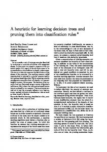
Fig. 1. Examples of different convolutional kernels: commonly used kernels (left) and the kernels obtained with the proposed algorithm (right). The algorithm finds the most informative kernels in a supervised manner, discovering meaningful kernels that look like gaussian blur, edge filters, corner and junction detectors, texture filters, etc.

Convolutional Decision Trees for Feature Learning and Segmentation

2 2.1

3

Related work Feature learning

The problem of feature construction is broadly discussed in the computer vision community. Standard or commonly used features are developed to face as many computer vision applications as possible. Different filters [1], SIFT [15] and HoG features [24] are only the few examples of such features. Even though these features work great for some tasks, they are unable to adapt to the specific problems and, therefore, often do not encode all the relevant information. For some applications experts are able to formalize the desired properties of the object patches based on the local appearance. For such applications domainspecific features can be developed. Line filter transform [19] is used for blood vessels segmentation, context cue features [2] – for synapse detection. Domainspecific features proved to be very informative, however the development of these features is time-consuming and expensive while not always possible and it does not generalize to other domains. In contrast, the proposed algorithm learns features in a supervised manner and therefore adapts to the specific application without any prior information. Unsupervised feature learning overcomes the domain-specificity, as this approach generates features based on the data itself. The “bag of visual words” representation [22] and dictionary learning [11] for sparse coding are procedures that fall in this category together with denoising autoencoders [21]. Even though these methods are powerful for data-representation, compression and image restoration, they exhibit serious limitations when applied to segmentation. This phenomenon happens because neither of the methods rely on the information about the label of the pixels and therefore learns reconstructive, not discriminative representations. Supervised feature learning, in contrast, learns the features of the data jointly with learning the classification functions. Sparse coding algorithm can be adapted to this procedure [16], but only with classification functions limited to linear and bilinear models. Convolutional Neural Networks (CNN) [13] are able to learn more complex classification functions and more complex feature representation. CNN, as discussed in the introduction, is a very powerful and flexible technique yet with one major disadvantage: computational time for training. For example, for neuronal segmentation dataset [6], the authors of [7] use CNN that achieves impressive accuracy, but that trains for almost a week using specially developed GPU cluster. In contrast the proposed method combines the flexibility of arbitrary convolutional kernels with the speed of decision tree training. Depending on the task first reasonable results for smaller trees can be obtained within one hour, while larger trees produce state of the art results in less than 12 hours training with one CPU which makes this method feasible for ”plug-and-play” experiments. CNNs with the same training time (smaller CNNs or CNNs trained with different strategies) do not achieve comparable results. The description of the method is given in section 3.

4

2.2


Binary decision tree

Learning decision trees pursues the idea to consecutively split the data space into parts according to a predicate φ (s.t. φ(x) = 0 for points x in one half-space, and φ(x) = 1 for x in another half-space). The predicate is selected in such a way that it maximizes a task dependent measure of informativeness, e.g. Information Gain or Gini’s diversity index [5]. x ∈ Rd is a vector of features or attributes of the object: xj represent j-th feature of the object. Decision trees most commonly are univariate [5]. Formally that means that the form of the predicate is limited to φ(x) = [xj > c]. Here [statement] denotes Iverson brackets which equals to 1 if statement is true and zero otherwise. j and c are the parameters of the split. The choice of only univariate splits limits the computational complexity and it allows us to efficiently find the most informative split. However, it has been demonstrated that in many cases univariate trees require many more splits to learn a classifier and lead to results that are difficult to interpret [10]. Therefore multivariate (oblique) trees were proposed [20, 5, 10], that allow the predicate to be more flexible: φ(x) = [xT β > c]. Here xT β is a linear combination of the attributes, β ∈ Rd and c are the parameters of the split. Depending on the criteria of informativeness, most algorithms only return locally optimal splits. The proposed algorithm develops the idea of oblique trees for learning convolution kernels in the context of image segmentation problems. Through regularization it incorporates the structural information about the spatial neighborhood of the pixels. Introducing this regularization helps the learned splits to be more interpretable and the optimization problem to be more robust.

3

Proposed method

Notation. As a training set we assume K pixels i ∈ {1, . . . , K} with associated binary labels yi ∈ {−1, 1}. Local pixel appearance is described with a patch around it. Let the size of a patch be w × w, then each pixel i is represented with w2 intensities of the pixels in the patch. In homogeneous coordinates, pixel i is 2 described by a vector xi ∈ Rw +1 with xi,1 ≡ 1. All the vectors stored row-wise 2 form a data-matrix X ∈ RK x w +1 , X = [x1 , . . . , xK ]T . The main idea of the method is to find a smooth convolution kernel that would be informative and discriminative for separating one class from another. A kernel of a convolution is again a w × w matrix. We also extend a vectorized kernel with a shift parameter b for the predicate. We define vector β to encodes 2 both shift and kernel parameters: β ∈ Rw +1 , β1 ≡ b and β2:w2 +1 encodes the kernel of the convolution. The predicate form can be now defined as φ(xi , β) = [β T xi > 0]. As here we care about the sign of the convolution, we also introduce the constraint ||β||22 = 1 to overcome the disambiguities induced by different scalings.


3.1

5

Information Gain

We want to estimate the parameter vector β that would maximize the information gain IG(β). Information gain depends on the distribution of positive and negative samples before and after a split withPthe predicate φ. Let’s define P as the number of all positive samples: P = i [yi = 1], N = K − P — the number of negative samples. After the split, the half-space, where φ(x, β) = 1, P will P contain p positive and n negative samples: p = i [φ(xi , β) = 1, yi = 1], n = i [φ(xi , β) = 1, yi = −1]. Both p and n depend on the parameters β. Then ˆ (P, N ) − H ˆ β (P, N, p, n) , IG(β) = H where ˆ (P, N ) = H H

N P , P +N P +N

(1)

ˆ (p, n) + P + N − p − n H ˆ (P − p, N − n) ˆ β (P, N, p, n) = p + n H H P +N P +N And H denotes the entropy: H(q0 , q1 ) = −q0 log2 q0 − q1 log2 q1 . Then the problem of finding the most informative split is formalized as follows: β ∈ arg max IG(β)

(2)

β

Unfortunately, the maximum of IG(β) cannot be found efficiently because of discontinuity in φ(xi , β) as it contains an indicator function [β T xi > 0]. To overcome this issue we use an approximation from [17]: 1 (3) 1 + exp(−αβ T xi ) P P We also introduce pˆα = i:yi =1 φˆα (xi , β), n ˆ α = i:yi =−1 φˆα (xi , β). Then the information gain can be approximated with φˆα (xi , β) =

ˆ α (β) = H ˆ (P, N ) − H ˆ β (P, N, pˆα n IG ˆα) It is easy to see that φˆα (xi , β) converges to φ(xi , β) in the limit α → ∞. Also pˆα and n ˆ α converges to p and n, respectively. This asymptotics renders it possible to solve the original problem (2) by estimating a limit process, i.e., we investigate the sequence of solutions of a relaxed problem for increasing α: ˆ α (β) β ∈ arg max IG(β) = lim arg max IG β

3.2

α→+∞

β

Regularization

Maximizing the information gain with respect to β usually results in a split that separates the classes, but unfortunately not interpretable (see for example figure 2). More than that, when the number of training samples goes to the range of O(w2 ) (approximately equals to the number of parameters), the linear split

6


Fig. 2. Examples of convolution kernels learned with different regularization parameters λ. Each row represents a kernel from different levels of CDT (respectively from 1 to 4). Each column stands for different regularization parameters: 0.001, 0.01, 0.1, 0.5, 2, 10. Increasing regularization helps the learned features to be more interpretable (compare first columns with the last ones). However, increasing λ too much results in smoothing out relevant information (for example the orientation of the third kernel disappears in the last two columns).

model starts to overfit. This problem requires us to introduce a regularization parameter λ that penalizes the complexity of the learned kernel parameters β. We want to assure that the kernel is smooth, and, therefore, we penalize the gradient of the kernel: ˆ α (β) − λ||Γ β||22 βα ∈ arg max Lα (β) with Lα (β) = IG β

(4)

2

Here Γ ∈ R2w(w−1) x (w +1) is a matrix of a 2D differentiation operator in a vectorized space, that is a Tikhonov regularization matrix. Regularization serves two main goals. First of all, it guarantees interpretability of the kernels learned (see figures 1 and 2). And second, from an optimization point of view, a strictly concave regularization term steers the gradient descent optimization algorithm out of local minima. 3.3

Optimization

In practice, we need to choose an initial point and the gradient of the functional to effectively find a solution of the problem 4. As initial point, we use the solution to a simple regularized linear regression: β0 = arg min β

1 ||Xβ − Y ||22 + λ||Γ β||22 K

(5)

Here Y = [y1 , . . . , yK ]T is a vector of all the responses and Γ denotes a Tikhonov matrix associated with the regularization above. The analytical solu−1 T 1 tion to problem (5) is equal to β0 = K X T X + λΓ T Γ X Y. The derivative of the functional Lα (β) in (4) can be also found analytically: dLα 1 X α exp(αβ T xi ) = xi dβ P + N i (1 + exp(αβ T xi ))2 [yi = 1] log2

− log2

p n + [yi = −1] log2 P −p N −n

p+n + P +N −p−n ! − 2λΓ T Γ β

(6)


7

As an optimization algorithm, we employ Quasi-Newton Limited-memory BFGS (L-BFGS) [18] that estimates Hessian with low-rank approximation and, therefore, selects optimal step size. Assuming optimization procedure as a subroutine L-BFGS, we sketch the algorithm that finds one split by learning the most informative convolution kernel in algorithm 1. We do not directly estimate the limit in eq. (2), but instead we iteratively increase α and initialize the optimization procedure in the next step with the solution in the previous step. Algorithm 1 Function findSplit for learning the most informative split Require: training samples xi , i = 1, . . . , K with classes yi ; λ −1 T 1 β0 := K X T X + λ2 Γ T Γ X Y . initialize with MSE solution 2 β0 := β0 /||β0 ||2 . project on the unit sphere Set α := 1 repeat α (·), βα−1 ) . find arg maxβ Lα (β) βα := L-BFGS(Lα (·), dL dβ 2 βα := βα /||βα ||2 . project on the unit sphere α := α + 1 until ||βα − βα−1 ||22 < OR α > MaxIterations return βα

4

Decision trees

How can we use the procedure findSplit to build a classifier? A well-known idea is to recursively split the data space into parts. The recursion stops when we achieve certainty about the label of every part. All the sequential splits end up being encoded in a binary decision tree. The idea is very straightforward, so we do not discuss it in details, except for one important question. So far we defined the regularization parameter λ for only one split, but in principle we can change it from split to split, or from one layer of the tree to the next. Experiments show that just fixing one parameter λ to be the same for every split in a tree often results in kernel overfitting as the tree grows large. Assume that we want to find two splits in two different parts A and B with volumes respectively V ol(A) and V ol(B). The relation between λA and λB for this two problems can be established from the following intuition: we want the 1 range of both problems to be the same: for the data part K ||Xβ − Y ||22 and 2 for the regularization part λ||Γ β||2 . With some assumptions and derivations that are out of scope of this paper, we provide the following heuristic rule: 2/(w2 +1) ol(A) λB = λA VV ol(B) . We approximate this ratio with just the fraction of the data points falling into each of the compacts A and B. The final recursive algorithm for building the convolutional decision tree is sketched in algorithm 2.

8


Algorithm 2 Function buildTree for decision tree construction Require: P set of indices I, λ,PMaxSamples P := i∈I [yi = 1]; N := i∈I [yi = −1] P treeStruct.answer = P +N if P < MaxSamples or N < MaxSamples then . terminal node, stop recursion treeStruct.left = null; treeStruct.right = null else . split recoursively β := findSplit(xi , yi , ∀i ∈ I; λ) Ileft := {i ∈ I : β T xi > 0}; Iright := {i ∈ I : β T xi