Hindawi Journal of Electrical and Computer Engineering Volume 2018, Article ID 9373210, 7 pages https://doi.org/10.1155/2018/9373210
Research Article Convolutional Recurrent Neural Networks for Observation-Centered Plant Identification Xuanxin Liu , Fu Xu
, Yu Sun , Haiyan Zhang , and Zhibo Chen
School of Information Science and Technology, Beijing Forestry University, Beijing 100083, China Correspondence should be addressed to Fu Xu;
[email protected] and Yu Sun;
[email protected] Received 17 December 2017; Accepted 8 February 2018; Published 8 March 2018 Academic Editor: Ping Feng Pai Copyright © 2018 Xuanxin Liu et al. This is an open access article distributed under the Creative Commons Attribution License, which permits unrestricted use, distribution, and reproduction in any medium, provided the original work is properly cited. Traditional image-centered methods of plant identification could be confused due to various views, uneven illuminations, and growth cycles. To tolerate the significant intraclass variances, the convolutional recurrent neural networks (C-RNNs) are proposed for observation-centered plant identification to mimic human behaviors. The C-RNN model is composed of two components: the convolutional neural network (CNN) backbone is used as a feature extractor for images, and the recurrent neural network (RNN) units are built to synthesize multiview features from each image for final prediction. Extensive experiments are conducted to explore the best combination of CNN and RNN. All models are trained end-to-end with 1 to 3 plant images of the same observation by truncated back propagation through time. The experiments demonstrate that the combination of MobileNet and Gated Recurrent Unit (GRU) is the best trade-off of classification accuracy and computational overhead on the Flavia dataset. On the holdout test set, the mean 10-fold accuracy with 1, 2, and 3 input leaves reached 99.53%, 100.00%, and 100.00%, respectively. On the BJFU100 dataset, the C-RNN model achieves the classification rate of 99.65% by two-stage end-to-end training. The observation-centered method based on the C-RNNs shows potential to further improve plant identification accuracy.
1. Introduction With the development of computer technology, there is increasing interest in the image-based identification of plant species. It can get rid of the dependence on the botany professionals and help the public identify plants easily. With the growth of demand, a growing number of researchers began to focus on plant identification and developed various sophisticated models. Traditional automated plant identification builds classifiers on top of hand-engineered features whose objects are flowers, leaves, and other organs. For example, Lee et al. [1] designed a mobile system of flower recognition using color, texture, and shape features and the accuracy was 91.26%. Furthermore, more studies considered the features of leaves. Novotn´y and Suk [2], Zhao et al. [3], Liu et al. [4], and Li et al. [5] extracted shape features of leaves to recognize the plant species using the nearest neighbor (NN) classifier, the back propagation (BP) neural network classifier, and the support vector machine (SVM) classifier, respectively. En and Hu [6], Liu and Kan [7], and Zheng et al. [8] used shape
and texture features of leaves to identify the plants with the base classifier, deep belief network (DBN) classifier, and SVM classifier, respectively. Wang et al. [9] extracted a series of color, shape, and texture features from 50 foliage samples, and the accuracy identified by SVM classifier was 91.41%. Gao et al. [10] calculated the comprehensive similarity of geometric features, texture features, and corner distance matrix to recognize plant leaves and the accuracy on the Flavia dataset was 97.50%. Chen et al. [11] extracted the distance matrix and corner matrix of leaves and identified plant leaves in the top 20 of the highest similarity result set chosen by the kNN classifier. The accuracy on Flavia dataset reaches 99.61%. The handcrafted feature extractor is time-consuming and relies on the expertise to a certain extent; it also has poor generalization ability to big data. Therefore, conventional methods of plant identification are not suitable for images with huge species and complex background. Developments in deep learning have made significant contribution to in-field plant identification. Deep learning is a machine learning method that extracts features automatically from raw data supervised by an
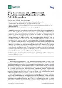
2 end-to-end training algorithm. It has been applied to the field of plant identification in recent years. Dyrmann et al. [12] used the CNN to identify weeds and crops at the early growth stages and achieved 86.2% average accuracy rate. Grinblat et al. [13] used deep learning for leaf identification of white bean, red bean, and soybean and the accuracy was 92.6 ± 0.2%. Zhang and Huai [14] used the CNN to identify the leaves of the self-expanding dataset based on the PlantNet dataset. The accuracy using the SVM classifier and the softmax classifier was 91.11% and 90.90% in simple background and 31.78% and 34.38% in complex background, respectively. Ghazi et al. [15] used three deep learning networks, that is, GoogLeNet, AlexNet, and VGGNet, to identify species on the LifeCLEF 2015 dataset and the overall accuracy of the best model was 80%. Sun et al. [16] designed a 26-layer deep learning model consisting of 8 residual building blocks for large-scale plant classification in natural environment and the recognition rate reached 91.78% on the BJFU100 dataset. The LifeCLEF plant identification challenge plays an important role in the field of plant automation recognition. The 2017th LifeCLEF plant identification challenge provides 10.000 plant species illustrated by a total of 1.1 M images. The winner of the challenge combined 12 trained models with four GoogLeNet, ResNet-152, and ResNetXT CNN models on three kinds of datasets. The Mean Reciprocal Rank (MRP) is 0.92 and the top 1 accuracy is 0.885 [17]. The previous studies identify plants from a single image (i.e., perform the image-centered plant identification). Although these methods are straightforward, they are not consistent with human cognitive habits. A series of factors like seasonal color changes, shape distortion, leaf damage, and uneven illumination cause significant intraclass variances. In fact, botanists often observe plants from multiple views or varied specimens, because the combination of multiple views can effectively improve the recognition accuracy. To circumvent the limitations of image-centered identification, observation-centered identification is proposed to mimic human behaviors. Each observation includes several images of the same species with different views. The convolutional recurrent neural networks (C-RNNs) are trained end-toend to automatically extract and synthesize features in one observation. The recognition accuracy on the Flavia and BJFU100 datasets is further improved by the C-RNN models.
2. The Proposed Method Almost all public image datasets are image-centered, while the observation-centered data are constructed based on the image-centered dataset. So, the plant images of the same species taken in the nearby time and location are selected as one observation. The observation-centered training and testing sets are built using different sets of samples from an image-centered dataset. To improve the generalization of the model, a sequence of images in the training set are permutated randomly. As shown in Figure 1, the C-RNN model inputs all images in one observation and outputs one prediction, which works in a many-to-one approach. The C-RNN model consists of CNN backbones and RNN units. The CNN backbones
Journal of Electrical and Computer Engineering Output
Output
FC (softmax)
FC (softmax)
V RNN W U FC (ReLU)
RNN
RNN
RNN
FC (ReLU)
FC (ReLU)
FC (ReLU)
CNN
CNN
CNN
CNN
Observation-centered sample
Image 1
Image 2
Image 3
Figure 1: The C-RNN model for observation-centered plant identification. The green arrows are the forward inference and the dashed red arrows are the truncated back propagation through time.
extract features from each image belonging to one observation, which include the residual network (ResNet) [18], InceptionV3 [19], Xception [20], and MobileNet [21]. Then, the RNN units including the simple RNN [22], Long Short Term Memory (LSTM) [23, 24], and Gated Recurrent Unit (GRU) [25] synthesize all features to implement observationcentered plant identification through the softmax layer. And the fully connected layer with the rectified linear unit (ReLU) connects the CNN backbones and the RNN units. Table 1 shows the MobileNet with GRU as the example to illustrate the network architecture. As the RNNs with fixed architecture are differentiable end-to-end, the derivative of the loss function can be calculated with respect to each of the parameters in the model [26]. The categorical cross-entropy loss is used in the C-RNN model for the multiclassification, and the loss function is defined to be 𝐿 = ∑𝐿 𝑡 (𝑦𝑛t , 𝑦̂𝑛t ) = −∑𝑦𝑛𝑡 log 𝑦̂𝑛𝑡 , 𝑡
𝑡
(1)
where 𝑦̂𝑛𝑡 is the 𝑡th element in the classification score vector 𝑦̂𝑛 , 𝑦𝑛𝑡 is the 𝑡th element in the classification label vector 𝑦𝑛 , and 𝑛 is the step size of RNN unit. The process of truncated BPTT is shown as the red dashed arrows in Figure 1, and the gradient calculation formulas for the weights 𝑉, 𝑊, and 𝑈 are expressed as follows [27]: 𝜕𝐿 𝜕𝐿 𝜕𝑦̂3 𝜕𝐿 𝜕𝑦̂3 𝜕𝑧3 = = = (𝑦̂3 − 𝑦3 ) ⊗ 𝑠3 , 𝜕𝑉 𝜕𝑦̂3 𝜕𝑉 𝜕𝑦̂3 𝜕𝑧3 𝜕𝑉
(2)
𝜕𝐿 𝜕𝐿 𝜕𝑦̂3 𝜕𝑠3 = , 𝜕𝑊 𝜕𝑦̂3 𝜕𝑠3 𝜕𝑊
(3)
𝜕𝐿 𝜕𝐿 𝜕𝑦̂3 𝜕𝑠3 = , 𝜕𝑈 𝜕𝑦̂3 𝜕𝑠3 𝜕𝑈
(4)
𝑧3 = 𝑉𝑠3 ,
(5)
𝑠3 = tanh (𝑈𝑥3 + 𝑊𝑠2 ) ,
(6)
where 𝐿 is the loss function, 𝑠 is the simplification of the RNN unit calculation process, and ⊗ is the outer product of two
Journal of Electrical and Computer Engineering
3 Table 1: C-RNN architecture.
Layer name
Input size
Output size
cnn 1
224 × 224 × 3
1 × 1024
cnn 2
224 × 224 × 3
1 × 1024
cnn 3
224 × 224 × 3
1 × 1024
3 × 1024 3 × 1024 1 × 128
3 × 1024 1 × 128 1 × 32
time distributed (fc) rnn (gru) fc (softmax)
Filter shape MobileNet Alpha = beta = 1 MobileNet Alpha = beta = 1 MobileNet Alpha = beta = 1 1024 × 1024 1024 × 128 128 × 32
vectors. Considering (6), 𝑠 is related to 𝑊 and 𝑈, and it can be deduced that 𝜕𝑠𝑡 𝜕𝑠 𝜕𝑠𝑡 𝜕𝑠𝑡−1 = 𝑡 + 𝜕𝑊 𝜕𝑊 𝜕𝑠𝑡−1 𝜕𝑊 2
= (1 − 𝑠𝑡 ) (𝑠𝑡−1 + 𝑊
𝜕𝑠𝑡−1 ), 𝜕𝑊
(7) (a)
𝜕𝑠 𝜕𝑠𝑡 𝜕𝑠 𝜕𝑠𝑡 𝜕𝑠𝑡−1 2 = 𝑡 + = (1 − 𝑠𝑡 ) (𝑥𝑡 + 𝑊 𝑡−1 ) . 𝜕𝑈 𝜕𝑈 𝜕𝑠𝑡−1 𝜕𝑈 𝜕𝑈 So, the gradients of 𝑊 and 𝑈 are expressed as follows [27]: 3 3 𝜕𝑠𝑗 𝜕𝑠 𝜕𝐿 𝜕𝑦̂3 𝜕𝐿 (∏ ) 𝑘, =∑ 𝜕𝑊 𝑘=0 𝜕𝑦̂3 𝜕𝑠3 𝑗=𝑘+1 𝜕𝑠𝑗−1 𝜕𝑊 3 3 𝜕𝑠𝑗 𝜕𝑠 𝜕𝐿 𝜕𝑦̂3 𝜕𝐿 (∏ ) 𝑘. =∑ 𝜕𝑈 𝑘=0 𝜕𝑦̂3 𝜕𝑠3 𝑗=𝑘+1 𝜕𝑠𝑗−1 𝜕𝑈
(8)
(b)
So, the C-RNN model can be trained end-to-end and the identification error is minimized by stochastic gradient descent with truncated back propagation through time (BPTT). (c)
3. Experiment and Results In this section, the method of constructing the observationcentered dataset is described in detail. Then, extensive experiments are conducted on the leaves observation-centered dataset with the combinations of different CNN backbones and RNN units to show a significant performance improvement compared with traditional transfer learning. 3.1. The Dataset. The leaves observation-centered dataset is based on the Flavia dataset [28]. There are 1,907 samples of 32 species in Flavia and each sample is an RGB leaf scan image with white background. All of the images for the same class were taken in the same experimental environment, so they could be thought of as the observation-centered data. Figure 2 shows the observation-centered example for leaves with different input numbers. To reduce variability and overfitting, 10-fold crossvalidation is adopted. The dataset is divided into 10 complementary subsets randomly. In one fold of the experiment, one
Figure 2: Observation-centered sample with (a) one, (b) two, and (c) three leaves. Samples containing less than three leaves are padded with zero.
subset is randomly chosen as the test set and the rest belong to the training set. Considering the size of the dataset, there are 1717 images for training and 190 images for test in the first 9 folds and there are 1710 images for training and 197 images for test in the 10th fold. To simulate collection of multiple leaves from one tree, each image is combined with 0 to 2 randomly chosen leaves of the same species to construct one observation-centered sample. The observation-centered samples with less than 3 leaves are padded with 0 (as shown in Figure 2). All leaves in the test set are held out from the training set for each fold. 3.2. Results. The models are implemented by the deep learning framework Keras [29] with TensorFlow [30] backend. All the experiments were conducted on an Ubuntu 16.04 Linux
4
Journal of Electrical and Computer Engineering 1.00
1.000
10-fold test accuracy
10-fold test accuracy
0.95 0.90 0.85 0.80 0.75
0.998 0.996 0.994 0.992
0.70 Simple RNN
LTSM
0.990
GRU
Simple RNN
1.000
1.000
0.998
0.998
0.996 0.994 0.992 0.990
GRU
LTSM
GRU
(b)
10-fold test accuracy
10-fold test accuracy
(a)
LTSM
0.996 0.994 0.992
Simple RNN
LTSM
GRU
0.990
Simple RNN
(c)
(d)
Figure 3: Effects of (a) ResNet50, (b) InceptionV3, (c) Xception, and (d) MobileNet CNN with three different RNN units on the 10-fold test accuracy. The pentagrams in (b), (c), and (d) represent the outlier of the results.
server with an AMD Ryzen 7 1700x CPU (16 GB memory) and an NVIDIA GTX 1070 GPU (8 GB memory). The batch size for each network is 32, the learning rate is 0.0001, and the optimizer is RMSprop in training phase. The test accuracy is compared after 50 epochs. 3.2.1. Effects of RNN Units and CNN Backbones. To explore the best RNN units, the models are implemented with different RNN units: simple RNN, LTSM, and GRU. Besides, the effects of different CNN backbones are also considered. Four state-of-the-art CNN backbones—ResNet50, InceptionV3, Xception, and MobileNet models—are pretrained on the ImageNet dataset with 1.2 million images of 1000 classes. Then, the last fully connected layers are replaced by the aforementioned RNN units. Figure 3 shows the 10-fold test accuracy of each CNN with 3 different RNN units at the last epoch. All of the RNN units work well with InceptionV3, Xception, and MobileNet, and the test accuracy is close to 100%; only several outliers exist as Figures 3(b), 3(c), and 3(d) indicate. The effect of ResNet50 was marginal due to the unstable convergence and the test accuracy is about 80% as shown in Figure 3(a).
Table 2: 10-fold test mean accuracy with different CNN and RNN units. ResNet50 InceptionV3 Xception MobileNet
Simple RNN 0.7987 1.0000 0.9989 0.9995
LTSM 0.8276 0.9995 0.9995 1.0000
GRU 0.7973 0.9995 1.0000 1.0000
To explore the best combination of CNN and RNN, the means of 10-fold test accuracy at the last epoch are listed in Table 2. The combinations of InceptionV3 with simple RNN, Xception with GRU, MobileNet with LTSM, and MobileNet with GRU outperform the others. All of the four models achieve 100% mean accuracy. Considering that the InceptionV3 with simple RNN has 2,249,880 trainable parameters, the Xception with GRU has 2,545,056 trainable parameters, the MobileNet with LTSM has 1,644,064 trainable parameters, and the MobileNet with GRU has 1,496,480 parameters, the MobileNet with GRU model with fewer parameters is considered as the best model.
Journal of Electrical and Computer Engineering 1.00
2.0
0.90 1.5
0.85 0.80
1.0
0.75 0.5
0.70
1.00
0.65
0.0 40
50
Epoch Training loss Training accuracy Test accuracy
Figure 4: The mean of training loss, training accuracy, and test accuracy of the MobileNet with GRU model in one fold.
The MobileNet backbone for the best model has 27 convolutional layers counting depth-wise and pointwise convolutions as separate layers, and the width multiplier and the resolution multiplier are 1. The number of the FC layer units after MobileNet backbone is 1024 and the number of the GRU unit hidden nodes is 128. The total number of the network parameters is 4,725,344 and there are 3,228,864 untrained parameters. Figure 4 shows the training process of the best model. The training loss declines rapidly in the first 10 epochs and decreases slowly in the next 10 epochs, and then it approaches 0 at the 50th epoch. The training accuracy and test accuracy rise rapidly in the first 5 epochs and increase slowly in the next 5 epochs, and then they approach 1 finally. The increments in both training and test accuracy indicate that the model is not overfitted. 3.2.2. Comparison with Transfer Learning. To make a fair comparison, the MobileNet retrained by traditional transfer learning is compared to the MobileNet with GRU model when inputting 1 to 3 leaves. When the number of inputting leaves is smaller than 3, the extra input channels of the RNN units were filled with 0. Figure 5 shows the 50th epoch test accuracy. The 10-fold test mean accuracy of retrained MobileNet is 99.79%, and that of our model inputting 1 leaf, 2 leaves, and 3 leaves is 99.53%, 100.00%, and 100.00%, respectively. The result shows that the traditional transfer learning is better when inputting only 1 leaf, while the C-RNNs show advantage when observationcentered images are available. 3.2.3. Comparison with Non-End-to-End Method. In order to evaluate the effect of end-to-end training for the CRNN in the observation-centered identification, a comparative experiment with a non-end-to-end method, that is, majority voting, was carried out. Majority voting got 0.667 for the average classification score in LifeCLEF 2015 plant task [31]. The experiments have been performed on the BJFU100 [16] dataset. The BJFU100 dataset consists of 10,000
0.95 MobileNet with GRU (3 leaves)
30
0.96
MobileNet with GRU (2 leaves)
20
0.97
MobileNet with GRU (1 leaf)
10
0.98
MobileNet
0
0.99 10-fold test accuracy
0.95
10-fold mean test accuracy
10-fold mean training loss
2.5
5
Figure 5: The MobileNet with GRU model compared with traditional transfer learning.
Figure 6: Each column shows one observation-centered sample from the BJFU100 dataset.
images with 100 species of ornamental plants in Beijing Forestry University campus by a mobile phone. Two images of the same class taken in the nearby time and location are selected as one observation. Figure 6 shows the typical observation-centered samples selected from the BJFU100 dataset. The CNN uses the softmax classifier to identify one image at one time. Then, majority voting gives the final prediction by counting votes from all CNN predictions. The CNN in the majority voting is trained end-to-end on a single image, while the error of voting cannot be corrected by back propagation and stochastic gradient descent. The MobileNet is the CNN for both C-RNN and majority voting. Firstly, the MobileNet is trained on a single image of BJFU100 for 86 epochs with the test accuracy of 95.8%. The majority voting has no trainable parameters and directly inputs the prediction of MobileNet, while the CRNN model can be further fine-tuned by second-stage endto-end training. The trained MobileNet without the final layer is transferred into the C-RNN model for further 20-epoch
6
Journal of Electrical and Computer Engineering
Acknowledgments
0.995
This work was supported by the Fundamental Research Funds for the Central Universities (TD2014-01, TD2014-02, and 2017JC02).
Test accuracy
0.990 0.985 0.980
References
0.975
[1] H.-H. Lee, J.-H. Kim, and K.-S. Hong, “Mobile-based flower species recognition in the natural environment,” IEEE Electronics Letters, vol. 51, no. 11, pp. 826–828, 2015. [2] P. Novotn´y and T. Suk, “Leaf recognition of woody species in Central Europe,” Biosystems Engineering, vol. 115, no. 4, pp. 444– 452, 2013. [3] C. Zhao, S. S. F. Chan, W.-K. Cham, and L. M. Chu, “Plant identification using leaf shapes - A pattern counting approach,” Pattern Recognition, vol. 48, no. 10, pp. 3203–3215, 2015. [4] J. Liu, F. Cao, and L. Gan, “Plant identification method based on leaf shape features,” Journal of Computer Applications, vol. 36, pp. 200–202, 2016. [5] Y. Li, H. Luo, G. Jiang, and H. Cong, “Online plant left recognition based on shape features,” Computer Engineering and Applications, vol. 53, pp. 162–165, 2017. [6] D. En and S. Hu, “Plant leaf recognition based on artificial neural network ensemble,” Acta Agriculturae Zhejiangensis, vol. 27, pp. 2225–2233, 2015. [7] N. Liu and J. Kan, “Plant leaf identification based on the multifeature fusion and deep belief networks method,” Journal of Beijing Forest University, vol. 38, pp. 110–119, 2016. [8] Y. Zheng, G. Zhong, Q. Wang, Y. Zhao, and Y. Zhao, “Method of Leaf Identification Based on Multi-feature Dimension Reduction,” Nongye Jixie Xuebao/Transactions of the Chinese Society for Agricultural Machinery, vol. 48, no. 3, pp. 30–37, 2017. [9] L. Wang, Y. Huai, and Y. Peng, “Method of identification of foliage from plants based on extraction of multiple features of leaf images,” Journal of Beijing Forest University, vol. 37, pp. 55– 61, 2015. [10] L. Gao, M. Yan, and F. Zhao, “Plant leaf recognition based on fusion of multiple features,” Acta Agriculturae Zhejiangensis, vol. 29, pp. 668–675, 2017. [11] M.-J. Chen, Z.-B. Chen, M. Yang, and Q. Mo, “Research on tree species identification algorithm based on combination of leaf traditional characteristics and distance matrix as well as corner matrix,” Beijing Linye Daxue Xuebao/Journal of Beijing Forestry University, vol. 39, no. 2, pp. 108–116, 2017. [12] M. Dyrmann, H. Karstoft, and H. S. Midtiby, “Plant species classification using deep convolutional neural network,” Biosystems Engineering, vol. 151, pp. 72–80, 2016. [13] G. L. Grinblat, L. C. Uzal, M. G. Larese, and P. M. Granitto, “Deep learning for plant identification using vein morphological patterns,” Computers and Electronics in Agriculture, vol. 127, pp. 418–424, 2016. [14] S. Zhang and Y. Huai, “Leaf image recognition based on layered convolutions neural network deep learning,” Journal of Beijing Forestry University, vol. 38, pp. 108–115, 2016. [15] M. M. Ghazi, B. Yanikoglu, and E. Aptoula, “Plant identification using deep neural networks via optimization of transfer learning parameters,” Neurocomputing, vol. 235, pp. 228–235, 2017. [16] Y. Sun, Y. Liu, G. Wang, and H. Zhang, “Deep Learning for Plant Identification in Natural Environment,” Computational
0.970 0.965 2
5
8
11 Epochs
14
17
20
Majority voting MobileNet with GRU
Figure 7: The test accuracy of C-RNN evolves as training advances.
end-to-end training. The training parameters and networks parameters are the same as the above experiments except that the batch size is changed to 16. The single MobileNet, majority voting, MobileNet with simple RNN, MobileNet with LSTM, and MobileNet with GRU achieve the test accuracy of 95.8%, 98.95%, 99.55%, 99.35%, and 99.65%, respectively. Figure 7 shows the function of the test accuracy of MobileNet with GRU and the majority voting during training. The C-RNN model trained by twostage end-to-end training outperforms the majority voting method by 0.7%.
4. Conclusions In this paper, the C-RNN models were proposed for observation-centered plant identification. The CNN backbones extract features and the RNN units integrate features and implement classification. The combination of MobileNet and GRU is the best trade-off of classification accuracy and computational overhead on the Flavia dataset. The test accuracy reaches 100%, while it has fewer parameters. Experiments on the BJFU100 dataset show that the C-RNN model trained by two-stage end-to-end training further improves the accuracy of majority voting method by 0.7%. The proposed C-RNN model mimics human behaviors and further improves the performance of plant identification, which has great potential in in-field plant identification. In the future work, an observation oriented dataset with a large amount of plants in an unconstrained environment will be constructed for further experiments.
Conflicts of Interest The authors declare that there are no conflicts of interest regarding the publication of this paper.
Journal of Electrical and Computer Engineering
[17]
[18]
[19]
[20] [21]
[22]
[23] [24]
[25]
[26]
[27]
[28]
[29] [30] [31]
Intelligence and Neuroscience, vol. 2017, Article ID 7361042, 6 pages, 2017. H. Go¨eau, P. Bonnet, and A. Joly, “Plant identification based on noisy web data: the amazing performance of deep learning (LifeCLEF 2017),” in Proceedings of the CLEF 2017 CEUR-WS, 2017. K. He, X. Zhang, S. Ren, and J. Sun, “Deep residual learning for image recognition,” in Proceedings of the 2016 IEEE Conference on Computer Vision and Pattern Recognition, CVPR 2016, pp. 770–778, July 2016. C. Szegedy, V. Vanhoucke, S. Ioffe, J. Shlens, and Z. Wojna, “Rethinking the inception architecture for computer vision,” in Proceedings of the 2016 IEEE Conference on Computer Vision and Pattern Recognition, CVPR 2016, pp. 2818–2826, July 2016. F. Chollet, “Xception: Deep Learning with Depthwise Separable Convolutions,” 1610.02357, https://arxiv.org/pdf/1610.02357.pdf. A. G. Howard, M. Zhu, B. Chen et al., “MobileNets: Efficient Convolutional Neural Networks for Mobile Vision Applications,” 1704.04861, https://arxiv.org/pdf/1704.04861.pdf. Y. Gal and Z. Ghahramani, “A theoretically grounded application of dropout in recurrent neural networks,” in Proceedings of the 30th Annual Conference on Neural Information Processing Systems, NIPS 2016, pp. 1027–1035, esp, December 2016. S. Hochreiter and J. Schmidhuber, “Long short-term memory,” Neural Computation, vol. 9, no. 8, pp. 1735–1780, 1997. F. A. Gers, J. Schmidhuber, and F. Cummins, “Learning to forget: Continual prediction with LSTM,” Neural Computation, vol. 12, no. 10, pp. 2451–2471, 2000. K. Cho, B. van Merrienboer, C. Gulcehre et al., “Learning Phrase Representations using RNN Encoder-Decoder for Statistical Machine Translation,” 1406.1078, https://arxiv.org/abs/ 1406.1078v3. Z. C. Lipton, J. Berkowitz, and C. Elkan, “A Critical Review of Recurrent Neural Networks for Sequence Learning,” 1506.00019v4, https://arxiv.org/pdf/1506.00019.pdf. Recurrent Neural Networks Tutorial. http://www.wildml.com/ 2015/10/recurrent-neural-networks-tutorial-part-3-backpropagation-through-time-and-vanishing-gradients/. S. G. Wu, F. S. Bao, E. Y. Xu, Y.-X. Wang, Y.-F. Chang, and Q.L. Xiang, “A leaf recognition algorithm for plant classification using probabilistic neural network,” in Proceedings of the 2007 IEEE International Symposium on Signal Processing and Information Technology, pp. 11–16, Giza, Egypt, December 2007. Keras. https://keras.io/. tensorflow. https://www.tensorflow.org/. S. Choi, “Plant identification with deep convolutional neural network: SNUMedinfo at LifeCLEF plant identification task 2015,” in Proceedings of the 16th Conference and Labs of the Evaluation Forum, CLEF 2015, Toulouse, France, September 2015.
7
International Journal of
Rotating Machinery
Engineering Journal of
Hindawi Publishing Corporation http://www.hindawi.com
Volume 2014
The Scientific World Journal Hindawi Publishing Corporation http://www.hindawi.com
Volume 2014
International Journal of
Distributed Sensor Networks
Journal of
Sensors Hindawi Publishing Corporation http://www.hindawi.com
Volume 2014
Hindawi Publishing Corporation http://www.hindawi.com
Volume 2014
Hindawi Publishing Corporation http://www.hindawi.com
Volume 2014
Journal of
Control Science and Engineering
Advances in
Civil Engineering Hindawi Publishing Corporation http://www.hindawi.com
Hindawi Publishing Corporation http://www.hindawi.com
Volume 2014
Volume 2014
Submit your manuscripts at https://www.hindawi.com Journal of
Journal of
Electrical and Computer Engineering
Robotics Hindawi Publishing Corporation http://www.hindawi.com
Hindawi Publishing Corporation http://www.hindawi.com
Volume 2014
Volume 2014
VLSI Design Advances in OptoElectronics
International Journal of
Navigation and Observation Hindawi Publishing Corporation http://www.hindawi.com
Volume 2014
Hindawi Publishing Corporation http://www.hindawi.com
Hindawi Publishing Corporation http://www.hindawi.com
Chemical Engineering Hindawi Publishing Corporation http://www.hindawi.com
Volume 2014
Volume 2014
Active and Passive Electronic Components
Antennas and Propagation Hindawi Publishing Corporation http://www.hindawi.com
Aerospace Engineering
Hindawi Publishing Corporation http://www.hindawi.com
Volume 2014
Hindawi Publishing Corporation http://www.hindawi.com
Volume 2014
Volume 2014
International Journal of
International Journal of
International Journal of
Modelling & Simulation in Engineering
Volume 2014
Hindawi Publishing Corporation http://www.hindawi.com
Volume 2014
Shock and Vibration Hindawi Publishing Corporation http://www.hindawi.com
Volume 2014
Advances in
Acoustics and Vibration Hindawi Publishing Corporation http://www.hindawi.com
Volume 2014