COPING WITH TIME-VARYING DEMAND WHEN SETTING STAFFING REQUIREMENTS FOR A SERVICE SYSTEM
by
Linda V. Green
Peter J. Kolesar
Ward Whitt
Graduate School of Business Columbia University
[email protected]
Graduate School of Business Columbia University
[email protected]
IEOR Department Columbia University
[email protected]
Submitted: April 2005; Revision Accepted: October 2005 Prepublication version: January 2006.
Abstract We review queueing-theory methods for setting staffing requirements in service systems where customer demand varies in a predictable pattern over the day. Analyzing these systems is not straightforward, because standard queueing theory focuses on the long-run steady-state behavior of stationary models. We show how to adapt stationary queueing models for use in nonstationary environments so that time-dependent performance is captured and staffing requirements can be set. Relatively little modification of straightforward stationary analysis applies in systems where service times are short and the targeted quality of service is high. When service times are moderate and the targeted quality of service is still high, time-lag refinements can improve traditional stationary independent period-by-period and peak-hour approximations. Time-varying infinite-server models help develop refinements, because closedform expressions exist for their time-dependent behavior. More difficult cases with very long service times and other complicated features, such as end-of-day effects, can often be treated by a modified-offered-load approximation, which is based on an associated infinite-server model. Numerical algorithms and deterministic fluid models are useful when the system is overloaded for an extensive period of time. Our discussion focuses on telephone call centers, but applications to police patrol, banking and hospital emergency rooms are also mentioned. Keywords: staffing, call centers, time-varying demand, queues with time-varying arrival rate, nonstationary queueing models, police patrol, banking, hospital emergency rooms.
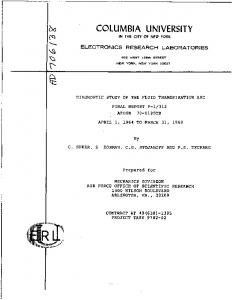
1. Introduction A common feature of many service systems – ranging from telephone call centers to police patrol and hospital emergency rooms – is that the demand for service often varies greatly by time of day. This is illustrated by the plot of hourly arrival rates from a financial-services call center in Figure 1, taken from Section 4 of Green, Kolesar and Soares (2001). In this paper we discuss ways to cope with that time-varying demand when setting staffing requirements. Since it helps to have a definite context in mind, we primarily focus on telephone call centers, where there already is a relatively high level of managerial control and sophistication, and extensive information-and-communication-technology (ICT) equipment, including automatic call distributors (ACD’s), personal computers and assorted databases. In many call centers, staffing is performed by workforce management (WFM) software, which processes data and performs simple queueing analyses. For background on call centers, see the survey by Gans et al. (2003). Many of our suggestions for call centers apply rather directly to other service systems, such as bank tellers, airlines ticket counters and tollbooths; e.g., see the classic toll-booth paper by Edie (1954). Moreover, the ideas apply in principle to other service systems, such as air-terminal queues (i.e., runways; Koopman 1972), police patrol (Green and Kolesar 1984a,b, 2500
2000
calls per hour
1500
1000
500
0
1
2
3
4
5
6
7
8
9
10
11
12
13
14
15
16
17
18
19
20
21
22
23
24
hour of day
Figure 1: Arrivals per hour to a medium-sized financial-services call center.
1
1989, 2004) and hospital emergency rooms (Green et al. 2002, 2005), but the complexities of these systems invite more research. At the end of the paper we discuss the implications of our proposals for staffing in other service systems, including police patrol and hospital emergency rooms. Organization of the Paper. In Section 2 we define the staffing problem and place it in context. In Section 3 we explain how stationary models can be used in a nonstationary manner to solve the staffing problem in the easiest cases - those systems with short service times and a high quality-of-service standard. In Section 4 we discuss refinements for harder cases with medium-to-long service times, but still with a high quality-of-service standard. We show how an associated infinite-server model can be used to develop and understand these refinements. In Section 5 we discuss the most difficult case, in which the system may be overloaded for an extensive period of time. In Section 6 we discuss staffing in other systems. In our final Section 7 we make concluding remarks, discussing extensions and other complications not addressed in the main paper, such as service systems with networks of facilities and systems with customer retrials.
2. The Staffing Problem One Decision in a Hierarchy of Decisions. Setting staffing requirements is one in a hierarchy of decisions that must be made in the design and management of a service system. In a long-term planning horizon, managers set the system capacity. That usually involves hardware choices; e.g., in a call center managers determine the number of possible agent positions and the amount and capacity of supporting ICT equipment. In an intermediate-time planning horizon, managers set the overall size of the workforce, making important hiring and training decisions. The (daily) staffing decision specifies the number of customer service representatives (agents) needed to work during each staffing interval over the day. After the staffing requirements are set, managers make agent scheduling decisions, specifying the number of agents to work on specific tours of duty, period by period, in conformance to the previously determined staffing levels, work rules and legal constraints. The scheduling decision is often determined by solving an integer linear program (Dantzig 1954, Segal 1974 and Kolesar et al. 1975). It is important to recognize that the staffing requirements could in principle be set by a larger algorithm that also addresses actual employee scheduling. In real time, managers often make further adjustments – flexing decisions, which move
2
agents in and out of the line of duty (to and from “offline” work). This is accomplished by having extra agents on site doing alternative work or being trained, or by being able to use remote agents on short notice. If flexibility can be achieved, then it is often possible to efficiently provide a very high quality of service (Whitt 1999a). In call centers, where the actual services required by customers are diverse and agent skills can be matched to them, we need to be concerned with the numbers of agents with different combinations of skills, not just the total number of agents. Telephone callers may speak different languages or may require special service. For example, we may need to ensure that enough agents are present to provide technical support in French and respond to billing inquiries in Spanish. When agents have different skills, staffing is intimately related to call routing. In this paper we act as if all agents can handle all calls, but at the end of the paper we indicate how the staffing methods for a single-skill call center can be applied to treat call centers with multi-skilled agents and skill-based routing. In many circumstances, the methods extend directly. Other Common Characteristics of Service Systems. Service systems have several other common characteristics: First, a “service” usually must be performed relatively soon after the service request is made; there typically is little opportunity to inventory or backorder service requests, although a moderate kind of backordering – waiting – is usually allowed. It may be possible to prioritize jobs. For example, incoming calls to a 911 phone line saying “shots heard, man with a gun” get an immediate police response, while a “noisy party” gets queued. Setting priorities provides managers the opportunity to better meet service goals at less expense (Whitt 1999b). Second, there is significant variation in arrivals around the temporal pattern; and significant variation in service times. One buys insurance against this uncertainty by overstaffing relative to the average demand and service rates. Hence it is natural to use a queueing model to compute the level of insurance needed. A Single Basic Queueing Model. Our discussion will be centered around a single basic queueing model: the Mt /GI/st + GI queue, which has a nonhomogeneous Poisson arrival process with a time-varying arrival-rate function λ(t) (the Mt ), independent and identically distributed (iid) service times following a general probability distribution (the first GI), a possibly time-varying number of servers on duty (agents, the st ), an unlimited waiting space, a
3
first-come first-served queueing discipline, and customer abandonment with iid times to abandon following a general probability distribution (the +GI). The assumption of independence among customer times to abandon is realistic when, as happens in most telephone call centers, customers wait in invisible queues, where they cannot directly observe the state of the system. As shown by Bolotin (1994) and Brown et al. (2005), service-time and time-to-abandon distributions tend to be non-exponential. They found the service-time distribution to be approximately lognormal, but the variability of the observed lognormal distributions was not too great. In particular, the squared coefficient of variation (SCV, variance divided by the square of the mean) was found to be between 1 and 2. (It is good to use the SCV instead of the variance, because it has meaning independent of the mean; the SCV of a random variable is unchanged if it is multiplied by a constant.) In such cases it is reasonable to use exponential distributions. In each new application the service-time distribution should be checked. We indicate what can be done if exponential distributions are not appropriate. As emphasized by Garnett et al. (2002), Mandelbaum and Zeltyn (2004, 2005) and Feldman et al. (2004), in most call centers, some waiting customers abandon (leave without receiving service after joining the queue). A high level of customer abandonment may be a sign of poor service; indeed it often implies lost sales. On the other hand, a low level of abandonment, such as 1%, in a large call center may be a sign of proper staffing, where supply appropriately balances demand. Regardless of the interpretation, it can be useful to recognize the presence of customer abandonment and explicitly include its impact on performance and hence on staffing. Even a small amount of customer abandonment can significantly impact system performance and staffing requirements. In the past, abandonments were not included in staffing models, primarily because they appeared to make the model too complicated. However, we will show how the model with customer abandonment can be analyzed, and how its impact upon performance can be determined. From a queueing-theory perspective, the Mt /GI/st + GI model is quite complicated, primarily because of the time-varying arrival rate, but actual call centers are often more complicated still, since they can have multiple customer classes, agents with different skills and networks of work sites. Although the Mt /GI/st + GI model does not address the full complexity of some actual call centers, it does permit us to analyze the impact of time-varying arrivals. Many of our ideas about how to cope with the time-varying arrival rate found from analyzing the Mt /GI/st + GI queue apply more generally. (We discuss this briefly in the concluding Section 7.) 4
The Goal in Staffing. For us, then, the staffing problem is the specification of the staffingrequirements function st - the number of agents required to be on duty as a function of time t which is the st term in the Mt /GI/st + GI queue. However, changes in the staffing are usually allowed only at certain times, e.g., once every fifteen minutes, once every hour, or in some cases, only once every eight hours. Thus, we wish to determine a good staffing function subject to the constraint that changes are allowed only at the ends of prescribed staffing intervals. Our goal is to minimize the total number of staff hours required over the day, while meeting a targeted level of service performance in each staffing interval. A common performance constraint is the service level: the requirement that x% of the calls be answered within y seconds. A commonly used standard is that 80% of the calls answered be within 20 seconds. Applied to a single time point, that means that the probability an arriving customer, who has unlimited patience, would have to wait no more than 20 seconds before starting service should be at least 0.80. (But, with customer abandonments, we want to properly account for the possible abandonment by customers waiting ahead of this waiting customer.) Closely related to service level is the delay probability, i.e., the probability that an arriving customer has to wait at all before starting service. That is a special case of service level in which y = 0 seconds. The delay-probability constraint is generally easier to compute, tends to be a relatively robust performance measure (insensitive to model details) and tends to have a meaning independent of scale (typical number of servers), We elaborate on the independence of scale in Section 3.3. Since customer abandonments are important and are measured automatically by modern call-center-management software, managers often place bounds on the abandonment rate, such as 4%. It is also common to constrain the expected waiting time (before starting service), which is called the Average Speed to Answer (ASA) by practitioners. (For a practice perspective on call center operations, see Cleveland and Mayben (1997).) Queueing theory helps link all four measures: service level, delay probability, abandonment rate and average speed to answer. Understanding these links can help diagnose difficulties in practice. In many situations it is important to pay attention to non-congestion-related performance measures: Doing bad things with little delay does not constitute good service. It is vital to handle service requests properly as well as promptly; we seek first-call resolution. The goal of extracting the maximum value from the customer interaction by using an agent matched to the customer needs, with appropriate system support, leads to notions of value-based routing and value-based staffing (Sisselman and Whitt 2004). 5
A Daily Cycle. Here we assume that the total time period is a day. That might be an eight-hour day, conforming to normal business hours, or a full twenty-four-hour day, such as occurs with 911 phone lines and other continually-available (24/7) call centers, or something in between. In any event, the common case is to have significant variation in the arrival rate over the course of the day, so that the peak arrival rate is much greater than the average arrival rate. (Demand patterns often vary enough by day of the week so that this must be explicitly accounted for as well.) A good example is the arrival-rate function depicted in Figure 1, based on empirical data from a financial-services call center. In Figure 1, each point is an average for a half-hour interval, multiplied by 2, to give the hourly rate. In that context, the average call holding time (service time) was about 6 minutes = 1/10 hour. Consequently, the instantaneous offered load (instantaneous arrival rate multiplied by the mean service time) would be 2000 × (1/10) = 200 if the arrival rate were 2000 calls per hour - which happens at about 9 am. Hence, to provide insurance against long delays, the required staffing at such times must exceed 200 agents. There also can be somewhat predictable bursts of arrivals, e.g., as occur in a call center responding to planned television advertising promotions. There may also be sudden peaks or other anomalous behavior in the arrival-rate function at the beginning of the day, at noon time, or just prior to closing. There also can be unpredictable non-Poisson stochastic fluctuations, totally inconsistent with the nonhomogeneous-Poisson-process demand model we are assuming. Consider, for example, unexpected bursts of high demand in call centers serving brokerage customers when events of political or economic importance occur. Similarly, there are unexpected surges of demand for emergency responders in response to unanticipated largescale incidents. While there is a need to plan for such eventualities, such phenomena will not be considered in this paper. Model Fitting and Validation. The major step of model fitting and validation requires system data. However, service systems differ widely with regard to the availability of relevant data. Fortunately, call centers tend to fall into the data-rich category. We are in the midst of a technological revolution, making it ever more feasible and economical to be data-rich, but one still encounters some data-poor call centers. Data-poor environments are much more common in non-call-center applications. It can be important to facilitate economic transformation to a more data-rich environment by demonstrating the potential benefits of using better data in better models.
6
Here we do not focus on data analysis, but we do emphasize its importance. Unfortunately, there are few accounts of successful data analysis in the professional literature. However, Brown et al. (2005) is an excellent example of a statistical study of call-center data. Green and Kolesar (1984a, b, 1989) illustrate many data-analysis challenges in their use and validation of a queueing model of police patrol. Kolesar’s (1984) study of automatic teller machines (ATM’s) illustrates a case in the middle of the data-richness scale. An important model fitting activity is forecasting, which itself is a hierarchial process. We will assume that a specified arrival-rate function forecast λ(t) has been created. It is important to remember that forecasting is never perfect, so that there may be considerable uncertainty about the arrival-rate function λ(t). When this is true, there are two fundamental sources of uncertainty: (i) stochastic fluctuations in arrivals and service times, for given model parameters, and uncertainty about the model parameters themselves. Here we only consider the first form of uncertainty, but it can be important to consider both. For recent research on models incorporating both forms of uncertainty, see Whitt (1999, 2005e), Harrison and Zeevi (2005) and Bassamboo et al. (2005a,b). The Role of Simulation. A powerful time-tested approach to set staffing levels is to employ computer simulation (Anton et al. 1999, Brigandi et al. 1994 and Kwan et al. 1988). Simulation is especially useful to measure performance in systems that are so complex that they cannot be described by analytical queueing models. In data-rich environments, the simulation model can even be made an integral part of the data system, with specific models created and analyzed automatically as part of the data-analysis phase. For any given staffing function st , evaluating the performance of the Mt /GI/st + GI queue is relatively easy to do using computer simulation. But choosing a good staffing function is much more difficult, because there are usually a vast number of possibilities. For example, in a large call center with about 100 agents, there may be 20 available staffing-change points during a day and 20 reasonable candidate staffing levels at each of these times. That produces 2020 ≈ 1026 different staffing functions to consider. So one cannot explore all staffing functions with simulation in a naive manner. Fortunately, there often are alternative simple analytical methods that make it possible to focus in on a small number of attractive alternatives. We will describe them in the rest of the paper. In practice it is a good idea to simulate the system in some detail after the staffing requirements have been identified by approximate analytical approaches in order to verify that the suggested staffing levels indeed produce the desired
7
performance.
3. Applying Stationary Models to Nonstationary Systems Even though the arrival rate is highly time-varying, it may be possible to use stationary models to determine staffing requirements, but usually it is inappropriate to staff to the overall average arrival rate over the entire day; Green, Kolesar and Svoronos (1991) provide convincing numerical examples. On the other hand, it is often possible to use stationary models in a nonstationary manner - that is, chop time into segments and use a stationary model in each segment. This works well when the service times are short (e.g., 5−10 minutes) and the qualityof-service standard is high. Under those conditions, systems are rarely overloaded and staffing requirements follow easily predictable patterns. The common case is when staffing intervals are short (e.g. 15 − 30 minutes), but we will also briefly discuss longer staffing intervals (e.g, several hours or an entire day).
3.1. Short Staffing Intervals: PSA and SIPP A Long History. There is a long history of using queueing models to set staffing requirements for groups of telephone operators. In the early days of telephony, a human telephone operator set up each telephone call, so the classic “call center” was a group of telephone operators. There was a strong daily pattern to demand, the service times were very short, and the average offered load was quite high. Because of the large system scale (and prevailing workforce rules), it was possible and economical to have short staffing intervals, e.g., 15 or 30 minutes (Segal 1974). Similar situations emerged with the development of 800 numbers and telephone call centers. Even though the service times in these call centers are still short, they may experience high offered loads, and so may be even larger than the classical telephone operator group. For example, America On Line has a customer-support call center complex with over 10, 000 agents. The Pointwise Stationary Approximation. The classic case with short service times, a high quality-of-service standard and short staffing intervals is a solved problem, in that an effective analytic strategy is to use what has been called a pointwise stationary approximation (PSA) - PSA provides a time-dependent description of performance based on a stationary model, using the arrival rate and other parameters that prevail at each moment in time to describe the performance at that time.
8
Adjustments for the Staffing Intervals: Segmented PSA and SIPP. However, direct application of PSA does not take account of the staffing intervals. As described, the PSA approach yields a time-dependent staffing function that does not restrict changes to be at the boundaries of staffing intervals. Experiments show that (with short service times and a high quality-of-service standard), if you could staff in that fully time-dependent manner, you would produce a good staffing function. However, we are typically constrained to hold the staffing level constant during each staffing interval. Segmented PSA is a direct adjustment for the staffing-interval constraint - it works well when the staffing intervals are short: One generates the PSA-required staffing at each time t and then sets the staffing level to be the maximum of these staffing requirements over the staffing interval. Segmented PSA yields an upper bound on the required staffing, and tends to be effective for the case we are considering. Although segmented PSA may slightly overstaff, an initial staffing policy obtained by segmented PSA can easily be evaluated and refined by simulation. In practice, many commercial call-center-management software packages use a different approach: The arrival rate is first averaged over each staffing interval and this average is used in a stationary model. Green, Kolesar and Soares (2001) refer to this as the stationary independent period-by period (SIPP) approach. A common idea underlies the segmented-PSA and SIPP approaches: Both use a stationary independent period-by-period approach. However, segmented PSA first determines the staffing level at each time point, whereas SIPP first averages the arrival rate over the staffing interval. When the arrival-rate function does not fluctuate too greatly over staffing intervals, SIPP and segmented PSA yield similar results. (Segmented PSA will produce somewhat higher staffing levels.) For the classic case with short service times and short staffing intervals, SIPP does well provided that the arrival-rate function does not fluctuate too greatly within individual staffing intervals. Extensive experimental results evaluating the performance of SIPP as a function of model parameters are contained in Green, Kolesar and Soares (2001). They also propose several refinements to SIPP. One of these, SIPP Max, replaces the average arrival rate within each staffing interval by the maximum arrival rate within each staffing interval, which coincides with segmented-PSA. In practice, it is common that call-center-management software only estimates the average arrival rate over staffing intervals, so that the arrival-rate function must be taken to be constant during each staffing interval. For such piecewise-constant arrival-rate functions, segmented 9
PSA (or SIPP Max) and SIPP will be identical. We can thus interpret the experiments from Green, Kolesar and Soares (2001) as providing a strong case for fitting a more realistic smooth estimate to the actual arrival-rate function in the cases where this refinement might be beneficial.
3.2. Long Staffing Intervals: Busy-Hour Engineering and SPHA Now we discuss a second classic case, in which the service times are short and the quality-ofservice standard is high, but the staffing interval is long. For example, the staffing interval might be eight hours or even an entire day. This case is not common in call centers, but it can occur. (Police staffing frequently uses three eight-hour tours of duty.) A classical example is determining the required number of trunk lines needed in a telephone exchange. In trunking there is no provision for waiting – so a multi-server loss model is used. With long staffing intervals, there is an approach that reduces the problem to one with stationary demand. The idea lies in the requirement that satisfactory performance prevail at all times, so we staff (or set capacity) to meet the peak demand during the long staffing interval. That strategy led to busy-hour engineering (Bear 1980). Green and Kolesar (1995) refer to this approach as the simple peak hour approximation (SPHA). In some circumstances, system managers may staff to meet average performance over the long staffing interval, instead of peak performance. But, while this is tempting, it is dangerous since focusing on average performance leads to understaffing at peak times. This produces complicated congestion, taking us to the difficult case discussed in Section 5.
3.3. Staffing for a Stationary Model In the previous two subsections we observed that appropriate stationary models provide effective solutions to the classic staffing problems when service times are short and the quality-ofservice standard is high. Thus, to address staffing for the Mt /GI/st + GI model, it suffices to consider how to determine a staffing level s for the stationary M/GI/s + GI model. We discuss ways to do that now. Let λ denote the constant arrival rate. Let S denote a generic service time; let G denote its cumulative distribution function (cdf): G(t) ≡ P (S ≤ t), t ≥ 0, with mean µ−1 ≡ E[S]. An important quantity is the offered load a ≡ λE[S]. (The notation a follows traditional usage in telephony (Cooper 1982).) Numerical Methods.
We have made our original staffing problem less difficult by reducing 10
it to a series of staffing problems in a stationary model. This reduced stationary problem can be solved by simulation. Since the staffing problem must be addressed for each of the staffing intervals during the day, it is natural to use a (stationary) simulation model just once to generate a table of the required staffing levels s as a function of the candidate arrival rates λ - given all other model parameters. Such tables can be periodically updated whenever the other model parameters change. Instead of simulation, it is easier and, indeed, it is common practice to use the Erlang-C or M/M/s model for this purpose. Let Ws denote the steady-state waiting time before starting service, when there are s servers. This random variable has an exponential distribution, except for an atom at 0. Using the standard service-level performance target, we would choose s to satisfy P (Ws ≤ 20
seconds) ≥ 0.80 > P (Ws−1 ≤ 20 seconds) ,
(3.1)
which is easy to compute numerically. However, we may want to go beyond the M/M/s model. Experience indicates that the next most important generalization to consider is usually abandonment. Fortunately, good algorithms also exist for the Erlang-A or M/M/s+M model, which adds exponential abandonment times (Mandelbaum and Zeltyn 2005, Zeltyn and Mandelbaum 2005 and Whitt 2005a). The Service-Time Distribution. It is easy to model exponential service times, for we need only match the observed sample mean (average) of the service-time data, because the exponential distribution has only one parameter, which can be taken to be the mean. Indeed, experience indicates that the mean is the most important single parameter for any service-time distribution. But the exponential-service-time-distribution assumption should be validated by looking beyond the sample mean of the data. Experience indicates that the second most important parameter is the SCV c2s . We can estimate the SCV by estimating the variance as well as the mean, which in turn can be done by using the sample mean of the squares in addition to the sample mean. Since c2s = 1 for an exponential distribution, if cˆ2s ≤ 1, the exponentialdistribution assumption for the service times would be conservative. More generally, as a rough guideline, if c2s ≤ 2, then the exponential-distribution assumption for the service times tends to be a reasonable approximation. In practice, it is not difficult to estimate the service-time distribution by its empirical distribution and use that in a simulation of the resulting M/GI/s model to verify that the 11
performance captured by the exponential approximation is adequate: That procedure was illustrated by Kolesar (1984) in his study of queueing at automatic teller machines (ATM’s). The data there were consistent with a gamma distribution having c2s = 0.5. Simulation showed that the exponential assumption worked well. When the exponential assumption does not fit well, it may be advantageous and not too difficult to calculate the service level in (3.1) for a more realistic model. When the average offered load (and thus the required number of servers) is low, it is possible to apply numerical algorithms to calculate all desired steady-state performance measures in approximating Markovian M/P h/s and M/P h/s + P h models, which have both phase-type service-time and phase-type time-to-abandon distributions - usually with a small number of phases such as two (Seelen 1984, Seelen et al. 1985 and Takahashi and Takami 1976). Alternatively, we could use approximations, as in Whitt (1992, 1993). Again, these algorithms or formulas would be used only occasionally to produce tables of staffing levels as a function of arrival rates. On the other hand, at high average offered load, with large numbers of servers, the computational complexity of numerical algorithms grows. Fortunately, the service-time distribution beyond the mean tends not to matter much, provided that the service-time-distribution SCV is not too far from 1 (Mandelbaum and Schwartz 2002, Mandelbaum and Zeltyn 2004 and Whitt 2000, 2004a, 2005a,b). In particular, the probability of delay tends to be relatively insensitive to the service-time distribution beyond its mean. Certainly, it is now well recognized that the impact of the service-time distribution beyond its mean in a many-server queue is very different than in a single-server queue (where the impact is significant). As important theoretical reference points, we remark that the infinite-server M/GI/∞ and pure-loss M/GI/s/0 models have an insensitivity property: the steady-state distribution of the number of customers in the system depends on the service-time distribution only via its mean. Since abandonments tend to make the system behave like one of these models, the service-time distribution beyond the mean tends to matter less there as well. However, it is important to be aware that high variability in the service-time distribution can significantly impact the conditional waiting-time distribution, given that the customer is delayed, and thus the service-level measure (Whitt 1992, 1993, 2000, 2004a, 2005a,b). We do not expect that to occur, but we should check. The Time-to-Abandon Distribution. With abandonments in the model, we need to model the customer time-to-abandon (or patience) cdf, say F (t), the probability that any
12
customer would abandon before time t if his service does not start before that time. In practice, customer abandonments are more difficult to model than service times since the time-to-abandon distribution is hard to observe and the time-to-abandon distribution affects performance in a more complicated way than the service-time distribution. First, with abandonments there is censored data (Brown et al. 2005). Waiting customers end waiting in two different ways: by entering service or by abandoning. For the customers who enter service, we do not observe how long those customers would have been willing to wait before they abandoned; we only learn that they would have been willing to wait their observed waiting time before entering service. Thus we need to use statistical techniques for censored data Even more important, however, is the different way that the time-to-abandon distribution affects performance, especially in systems with a large number of servers and/or a high qualityof-service standard. In those situations, few customers wait in queue extremely long. Thus what is important about the time-to-abandon cdf is its value for small time arguments (Mandelbaum and Zeltyn 2004, 2005, Zeltyn and Mandelbaum 2005 and Whitt 2005a,c). Perhaps surprisingly, the mean and the tail of the time-to-abandon distribution matter little. Thus we do not want to estimate the mean and higher moments to fit a distribution to those parameters. Instead, from both perspectives - for effective estimation and for capturing what matters it is preferable to estimate the time-to-abandon cdf F by estimating its hazard-rate (or failurerate) function rF (t) ≡
f (t) , 1 − F (t)
t≥0,
(3.2)
where f is the probability density function (pdf) associated with the cdf F (p. 276 of Ross 2003). It gives the conditional density of an abandonment at time t, given that the customer has not abandoned up to time t. The cdf F can be recovered from the hazard-rate function rF by
Z
t
F (t) = 1 − exp {− 0
rF (u) du},
t≥0.
(3.3)
An important reference case is the exponential distribution, where the hazard rate function is constant. To estimate the cdf F via its hazard-rate function rF , suppose that time is divided into small subintervals, each containing an ample number of data points (abandonments). Then, let n ˆ A (c, d) be the number of observed abandonments in the subinterval [c, d) ≡ {t : c ≤ t < d} and let n ˆ W (c) be the number of customers that wait in queue at least time c before either
13
being served or abandoning. Then we estimate the hazard-rate function by rˆF (t) ≡
n ˆ A (c, d) , n ˆ W (c)(d − c)
c≤t