rate or FPr). The ROC curve is a useful tool to optimise the trade-off between. TPr and FPr. A loss matrix is often applied to these types of problems in an.
Cost-based classifier evaluation for imbalanced problems Thomas Landgrebe, Pavel Pacl´ık, David M.J. Tax, Serguei Verzakov, and Robert P.W. Duin Elect. Eng., Maths and Comp. Sc., Delft University of Technology, The Netherlands {t.c.w.landgrebe, p.paclik, d.m.j.tax, s.verzakov, r.p.w.duin}@ewi.tudelft.nl
Abstract. A common assumption made in the field of Pattern Recognition is that the priors inherent to the class distributions in the training set are representative of the true class distributions. However this assumption does not always hold, since the true class-distributions may be different, and in fact may vary significantly. The implication of this is that the effect on cost for a given classifier may be worse than expected. In this paper we address this issue, discussing a theoretical framework and methodology to assess the effect on cost for a classifier in imbalanced conditions. The methodology can be applied to many different types of costs. Some artificial experiments show how the methodology can be used to assess and compare classifiers. It is observed that classifiers that model the underlying distributions well are more resilient to changes in the true class distribution than weaker classifiers.
1
Introduction
Many typical discrimination problems can be expressed as a target versus nontarget class problem, where the emphasis of the problem is to recover target examples amongst outlier or non-target ones. ROC analysis is often used to evaluate a classifier [9], depicting the operating characteristic in terms of the fraction of target examples recovered (True Positive rate or T Pr ), traded off against the fraction of non-target examples classified as target (False Positive rate or F Pr ). The ROC curve is a useful tool to optimise the trade-off between T Pr and F Pr . A loss matrix is often applied to these types of problems in an attempt to specify decision boundaries well suited to the problem, as discussed in [2], and [1]. Both T Pr and F Pr are invariant to changes in the class distributions [10]. T Pr and F Pr are not always the only costs used in assessing classifier performance. Some applications are assessed with other cost measurements, typical ones including accuracy, purity/precision, and recall, discussed in [6], and [8]. An example of this could be in automatic detection of tumours in images, where a human expert is required to make a final decision on all images flagged by the classifier as target (called the Positive fraction or P OSf rac). In this application we could expect the number of target images (images actually depicting a
Training
Testing 6
6 4
4
NON−TARGET
TARGET
TARGET
Feature 2
Feature 2
0 −2 −4
NON−TARGET
2
2
0 −2 DECISION BOUNDARY
DECISION BOUNDARY
−4 −6
−6 −1
0
1 Feature 1
2
3
4
−1
0
1 Feature 1
2
3
Fig. 1. Scatter diagrams to illustrate the example for balanced training conditions (left 1 plot), but where the true class distribution is imbalanced (a prior of 10 with respect to the target class simulating a real class distribution), shown in the right plot. Data is generated by the Highleyman distribution as in [4], proposed in [7]
tumour) to be less abundant than non-target images, and consequently the recognition system would be expected to minimise the amount of manual inspection required by the expert post-classification. A high P OSf rac would result in an inefficient automatic system, resulting in a high manual cost. Cost-based measurements such as P OSf rac and purity are dependent on true class distributions (as opposed to T Pr and F Pr ) [5]. In some cases the actual distributions may be impossible to estimate or predict, implying that these costs may vary. It has been found that when non-target classes outnumber target classes, the effect on the costs of interest may be worse than expected [11], [8]. An example of this is shown in Figure 1 – here a balanced dataset is used for training (equal priors), but the right plot depicts the situation that arises when the true class distribution differs. Here the absolute number of non-target examples misclassified as target becomes comparable to the number of target examples correctly classified. In this paper we discuss the evaluation with respect to cost of two-class discrimination problems between target and non-target classes in which the true class distribution is imbalanced and may vary (i.e. the abundance of examples for the two classes differ, called skewing). This is an important practical question that often arises, discussed and demonstrated here using synthetic examples in which the costs can easily be understood and compared. The objective is to formulate a procedure for evaluating classification problems of this nature. We show that in some situations where the true class distribution is extremely skewed in favour of the non-target class, the costs measurements could degrade considerably. As an example of how the proposed rationale can be applied, we choose two costs that are important to many applications, namely T Pr and P OSf rac. Their relation is computed in conjunction with the ROC curve. These P OSf rac representations can be used to quickly, intuitively, and fairly, assess the outcome of the classifier for a given class distribution, or for a range of hypothetical class distributions (if it is unknown or varying). In a similar way, Purity or another cost measure could be used as part of the assessment procedure.
data
Classifier
POS
PSfrag replacements
TP
NEG
FP
pos output
�������� ���������������������� �������� �������� ���������������������� �������� �������� ���������������������� �������� �������� ����������� TN
FN
Fig. 2. A representation of the classification scheme discussed in this paper, showing a 2-class problem between a target and non-target class.
This paper is organised as follows: Section 2 introduces a theoretical framework, and shows how a classifier for the target versus non-target problem can be evaluated, discussing the construction of operating characteristics for the two costs emphasised here, namely T Pr and P OSf rac. Section 3 consists of a discussion of the effect that skewed class-priors can have on the costs. A few experiments are performed in section 4 to illustrate the concepts discussed in the paper, showing direct application of the proposed methodology. Conclusions are given in section 5.
2 2.1
Classifier evaluation between two classes Notation and problem formulation
Consider the representation of a typical classification problem in Figure 2. Here it can be seen that a trained classifier analyses each incoming example, and labels each one as either positive (P OS) or negative (N EG). After classifying objects, four different object classifications can be distinguished (see Table 1). Data samples labeled by the tested classifier as target (the P OSf rac) fall into two categories: true positives T P (true targets) and false positives F P (true non-targets). Corresponding true positive and false positive ratios T Pr and F Pr are computed by normalising T P and F P by the total amount of true targets Nt and non-targets Nn respectively. estimated labels target non-target true labels target TP FN non-target F P TN Table 1. Defining a confusion matrix
Data samples labeled by the classifier as non-target also fall in two categories, namely true negatives T N and false negatives F N . Note that T Nr = 1 − F Pr , and F Nr = 1−T Pr . The examples labeled by the classifier as target are denoted P OS, and those classified as non-target are denoted N EG. The fraction of objects which are positively labeled is the ‘Positive Fraction’, P OSf rac, defined in equation 1. P OS P OS = (1) P OSf rac = N P OS + N EG where N is the total number of objects in the test set. The fraction of examples in the P OS output of the classifier that are really target is called the P purity/precision of the classifier, defined as Purity = PTOS . T Pr can be written TP as (T Pr = T P +F N ), and is equivalent to Recall. A T Pr of 90% implies that 90% of all the target objects will be classified positive by the classifier (classified in the left branch in Figure 2). The P OSf rac tends to increase with T Pr for overlapping problems, indicating a fundamental trade-off between the costs. If P (C t ) is very low it would be expected that the P OSf rac will be very small. However it will be shown in the experiments that this is not always the case – overlapping classes and weak classifiers can result in a very undesirable P OSf rac, depending on the operating condition. 2.2
ROC analysis and P OSf rac analysis
Given a two class problem (target vs non-target), a trained density-based classifier and a test set, the ROC curve is computed as follows: the trained classifier is applied to the test set and the aposteriori probability is estimated for each data sample. Then, a set of thresholds Θ is applied to this probability estimate and corresponding data labelings are generated (this can be conceptualised as shifting the position of the decision boundary of a classifier across all possibilities). The confusion matrix is computed between each estimated set of labels and the true test-set labeling. The ROC curve now plots the T Pr as a function of the F Pr (see the left plot in Figure 3). Note that the ROC curve is completely insensitive to the class priors, depending only on the class conditional probabilities. When the prior of one of the classes is increased (and therefore the probability of the other class is decreased), both the T Pr and the F Pr stay exactly the same (for a fixed classifier), although the absolute number of target and non-target objects change. Costs dependent on class distribution such as P OSf rac are considered, the ROC curve alone is not sufficient to assess performance. In order to compute the corresponding P OSf rac operating characteristic for the classifier, the same set of thresholds Θ are used. Equation 1 can be written as equation 2, which can then be posed in terms of the ROC thresholds as in equation 3. P OSf rac =
TP + FP T P r Nt + F P r Nn TP + FP = = N TP + FP + FN + TN N
(2)
ROC plot
TPr vs Positive Fraction
1
1 0.9
0.8
0.8 0.1 0.7
TPr
0.6
TPr
0.6
0.4
0.5 0.4 0.3
0.2
0.2 0.1
0 0
0.2
0.4
0.6
0.8
1
0 0
0.2
FPr
0.4 0.6 Positive Fraction
0.8
1
Fig. 3. ROC and P OSf rac plots for a linear discriminant classifier applied to Highleyman data, where P (Ct ) = 0.1. Plots are made with respect to the target class.
T Pr (Θ)Nt + F Pr (Θ)Nn N Similarly the Purity cost can be derived as in Equation 4. P OSf rac(Θ) =
Purity(Θ) =
3
T P (Θ) T Pr (Θ)Nt = T P (Θ) + F P (Θ) T Pr (Θ)Nt + F Pr (Θ)Nn
(3)
(4)
The effect of class imbalance on classifier performance
P OSf rac and Purity are two costs that are dependent on the skewness (imbalance) of the true class distribution. Define the true prior probability for the target class as P (Ct ), and for the non-target class as P (Cn ). Equations 3 and 4 can be written in terms of prior probabilities as shown in equations 5 and 6 reP (Cn ) Nn Nn t spectively. Note that P (Ct ) = N N , P (Cn ) = N , and P (Ct ) = Nt = skewratio. P OSf rac(Θ) =
T Pr (Θ)Nt F Pr (Θ)Nn + = P (Ct )T Pr (Θ)+P (Cn )F Pr (Θ) (5) N N Purity(Θ) =
T Pr (Θ) T Pr (Θ) +
P (Cn ) P (Ct ) F Pr (Θ)
(6)
Interestingly it is clear from equation 5 that the P OSf rac tends to F Pr as the skew ratio increases, and thus for extremely low P (Ct ) the ROC representation could be used alone in depicting the trade-off between costs. Now given an actual class-distribution and an operating condition, the P OSf rac and Purity can be calculated. For example, the corresponding ROC and P OSf rac curves for the example in Figure 1 is shown in Figure 3 for a linear discriminant classifier. Here P (Ct ) = 0.1. It can be seen that for this condition, a T Pr of 80% would result in a P OSf rac of just under 30%. However, it could be that the exact class distribution is not known, and in fact sometimes the class distribution can vary from very small to extremely high levels. In these cases it can still be possible to evaluate and compare classifiers by investigating the operating characteristics across a range of priors in implementation. For example in the overlapping class
TPr vs Positive Fraction
TPr vs Positive Fraction
1
1
0.9
0.9
0.001 0.8
0.5
0.1
0.8 0.001 0.5
0.7
0.7
0.1
0.6 TPr
TPr
0.6 0.5
0.5
0.4
0.4
0.3
0.3
0.2
0.2
0.1 0 0
0.1 0.2
0.4 0.6 Positive Fraction
0.8
1
0 0
0.2
0.4 0.6 Positive Fraction
0.8
1
Fig. 4. P OSf rac plots for a linear discriminant (left plot) and quadratic discriminant (right plot) classifier applied to Highleyman data, where P (Ct ) = 0.5, 0.1, and 0.001. The values on each curve represent different true class distributions.
problem in Figure 1, if the actual class distribution is completely unknown, it could be of value to investigate the T Pr and P OSf rac operating characteristic for a range of operating conditions. In Figure 4 the operating characteristic is shown for P (Ct ) = 0.5, 0.1, and 0.001. The results for the linear classifier are shown in the left plot (the ROC plot remains constant as in the left plot of Figure 3). The right plot then shows the operating characteristic for a quadratic classifier under the same conditions. It is clear that this classifier is much more resilient to changes in the true class distribution. Clearly as the linear classifier reaches a T Pr of 75% for a P OSf rac of 0.1, the quadratic classifier is substantially better at over 90%. Considering the case at which the classifiers are set to operate at a T Pr of 80%, a balanced dataset results in a P OSf rac of 54.9%, and a Purity of 77.9% for the linear classifier. These may be acceptable results. However when the class distribution changes such that P (Ct ) = 0.01 (1 example in 100 is a target) the results become much worse. Whereas it could be expected that the P OSf rac should also drop by two orders of magnitude since the priors did so, for the linear classifier the P OSf rac only dropped to 24.8%. Conversely the quadratic classifier shows much better performance and resilience to changes of the true class distribution (in this case). The simple example discussed shows that even if the true class distribution is unknown (or varies), two classifiers can still be compared to an extent. This becomes more useful when the underlying structure of the data is unknown and the choice of classifier less obvious. One example of this type of problem is in the field of geological exploration where the prior probabilities of different minerals change geographically, and often only a range of true class distributions is known.
4
Experiments
A number of experiments on artificial data are carried out in order to illustrate the effect (and indeed severity) that skewed data can have on costs in a number of situations. Four different classifiers are implemented for each data set, trained using a 30-fold cross-validation procedure. Each classifier is trained with equal
TwoGaussians Experiment
Multimodal Experiment 12
4 TARGET
NON−TARGET
8
2
TARGET
TARGET
5
0 −1
Feature 2
6
1
Feature 2
Feature 2
Lithuanian Experiment 10
NON−TARGET
10
3
4 2
NON−TARGET
0
0
−2
−2
−3
−4
−5
−10
−6
−4 −2
0
2 Feature 1
4
6
−2
0
2 4 Feature 1
6
8
0
2
4
6 8 Feature 1
10
12
14
Fig. 5. Scatter diagrams of the 2-class experiments (the Highleyman plot is shown in Figure 1)
training priors. For each classifier an ROC plot is generated such as in Figure 3, as well as the T Pr versus P OSf rac relation for the same thresholds as the ROC plot, generated for the following class distributions (as in Figure 4): P (C t ) = 0.5, 0.1, and 0.001. Thus each classifier is assessed from the case of balanced class distribution, to cases where the sampling is extremely skewed. In order to easily compare results a case study is performed for each classifier to estimate the effect on cost when the T Pr operating condition is fixed at 80% (in the same way P OSf rac or Purity could be used as the independent variable as the specification for the classifier). This allows each classifier to be compared easily, but still keeping cognisant that the results are for a specific operating condition only1 . Note here that the objective of the classifier is to maintain the specified T Pr , and at the same time minimise the P OSf rac (and in some cases it could be more important to maximise Purity, but they are inversely dependent, i.e. a low P OSf rac results in a high Purity, since it can be shown 1 ). that P OSf rac = TNP Purity The following classifiers are trained and evaluated for each data set: Linear Discriminant (LDC), Quadratic Discriminant (QDC), Mixture of Gaussian (GAUSSM), trained using the standard Expectation-Maximisation procedure, and the Parzen Classifier, as in [3] where the width parameter is optimised by maximising the log-likelihood with a leave-one-out procedure. The classifiers range from low to high complexity, the complex ones hypothetically capable of handling more difficult discrimination problems. These are all density-based classifiers, capable of utilising prior-probabilities directly, and can be compared fairly. The datasets are illustrated in Figure 5, corresponding to the following experiments, where 1500 examples are generated for each class: TwoGaussians with two overlapping homogenous Gaussian classes with equal covariance matrices and a high Bayes error is high at around 15.3%; Highleyman consisting of two overlapping Gaussian classes with different covariance matrices according to the Highleyman distribution (as in the prtools toolbox [4]); Multimodal, a multi-modal dataset with two modes corresponding to the first class, and three to the second; Lithuanian where two rather irregular classes overlap. All are computed under the prtools library [4]. 1
A different operating point could for example be in favour of a different classifier.
Experiment P(Ct ) TwoGaussians 0.5 0.1 0.001 Highleyman 0.5 0.1 0.001 Multimodal 0.5 0.1 0.001 Lithuanian 0.5 0.1 0.001
LDC 46.08 ± 0.51% 18.94 ± 0.92% 12.22 ± 1.02% 52.14 ± 1.23% 29.85 ± 2.22% 24.33 ± 2.46% 69.00 ± 1.06% 60.21 ± 1.90% 58.03 ± 2.11% 46.81 ± 0.81% 20.26 ± 1.45% 13.68 ± 1.61%
QDC 45.99 ± 0.50% 18.78 ± 0.90% 12.05 ± 1.00% 40.00 ± 0.00% 8.00 ± 0.00% 0.08 ± 0.00% 50.25 ± 0.94% 26.46 ± 1.68% 20.57 ± 1.87% 42.10 ± 0.33% 11.77 ± 0.59% 4.27 ± 0.65%
MOGC 47.86 ± 0.77% 22.14 ± 1.38% 15.78 ± 1.53% 40.00 ± 0.00% 8.00 ± 0.00% 0.08 ± 0.00% 41.20 ± 0.22% 10.15 ± 0.40% 2.47 ± 0.45% 40.16 ± 0.04% 8.28 ± 0.07% 0.39 ± 0.08%
PARZEN 45.58 ± 0.54% 18.05 ± 0.98% 11.24 ± 1.08% 40.00 ± 0.00% 8.00 ± 0.00% 0.08 ± 0.00% 40.93 ± 0.21% 9.68 ± 0.38% 1.94 ± 0.42% 40.06 ± 0.04% 8.11 ± 0.07% 0.21 ± 0.08%
Table 2. P OSf rac results (with standard deviations shown) for the four data sets, where the classifiers are fixed to operate to recover 80% of target examples. Results are shown for three different class distributions.
4.1
Results of experiments
For conciseness only the case study results are presented, showing the effect on P OSf rac cost for a single operating point, across a number of different class distributions. However the ROC and P OSf rac representations for the linear classifier in the Highleyman experiment have been shown before in the left plots of Figures 3 and 4 respectively. Table 2 shows the P OSf rac results for the three different class distributions for the chosen operating point. In the TwoGaussians all the classifiers show an extreme effect on cost as the skewness is increased. The P OSf rac remains above 10% even when the distribution is such that only one example in a thousand are target. Here the overlap between the classes does not allow for any improvement (a high Bayes error). In the Highleyman experiment it can be seen that only the linear classifier is severely affected by different class distributions for the given operating condition. This experiment suggests that an inappropriate or weak classifier can be disastrous in extreme prior conditions, even though it may have seemed acceptable in training (classifiers are often trained assuming balanced conditions). The Multimodal experiment presented a multimodal overlapping problem, and as expected the more complex classifiers fared better. Whereas the linear and quadratic classifiers showed a P OSf rac of over 20% with extreme priors, the mixture-model and parzen classifiers performed a lot better. Similar results were obtained in the Lithuanian experiment.
5
Conclusion
This paper discussed the effect of imbalanced class distributions on cost, concentrating on 2-class problems between a class of interest called a target class, and a less interesting non-target class. A methodology was proposed in order to compare classifiers with respect to cost under conditions in which training con-
ditions are fixed (often balanced), and true class distributions are imbalanced or varying. It was shown that even though costs such as the true and false positive rates are independent of the true class distributions, other important costs such as P OSf rac and Purity are dependent on it. Thus for these types of problems we proposed that in addition to traditional ROC analysis, a similar analysis of the other costs should be made simultaneously, evaluating the effect of a changing class distribution. Following some simple experiments, it was observed that in some cases, classifiers that appeared to perform well on balanced class distribution data failed completely in imbalanced conditions. Conversely some classifiers showed resilience to the imbalance, even when extreme conditions were imposed. Thus we conclude that especially in cases in which the underlying data structure is complex or unknown, an analysis of the effect of varying and imbalanced class distributions should be included when comparing and evaluating classifiers.
6
Acknowledgements
This research is/was supported by the Technology Foundation STW, applied science division of NWO and the technology programme of the Ministry of Economic Affairs. Support was also provided by TSS Technology Research, De Beers Consolidated Mines, South Africa.
References [1] C.M. Bishop. Neural Networks for Pattern Recognition. Oxford University Press Inc., New York, first edition, 1995. [2] R. Duda, P. Hart, and D. Stork. Pattern Classification. Wiley - Interscience, second edition, 2001. [3] R.P.W. Duin. On the choice of smoothing parameters for parzen estimators of probability density functions. IEEE Trans. Computing, 25:1175–1179, 1976. [4] R.P.W. Duin. PRTools Version 3.0, A Matlab Toolbox for Pattern Recognition. Pattern Recognition Group, TUDelft, January 2000. [5] P. Flach. The geometry of roc space: understanding machine learning metrics through roc isometrics. ICML-2003 Washington DC, pages 194–201, 2003. [6] D. J. Hand. Construction and Assessment of Classification Rules, ISBN 0-47196583-9. John Wiley and Sons, Chichester, 1997. [7] W. Highleyman. Linear decision functions, with application to pattern recognition. Proc. IRE, 49:31–48, 1961. [8] M. Kubat and S. Matwin. Addressing the curse of imbalanced data sets: One-sided sampling. Proceedings, 14th ICML, Nashville, pages 179–186, July 1997. [9] C. Metz. Basic principles of roc analysis. Seminars in Nuclear Medicine, 3(4), 1978. [10] F. Provost and T. Fawcett. Robust classification for imprecise environments. Machine Learning, 42:203–231, 2001. [11] G.M. Weiss and F. Provost. The effect of class distribution on classifier learning: an empirical study. Technical report ML-TR-44, Department of Computer Science, Rutgers University, August 2 2001.