Dec 16, 2012 - PAVEL M. BLEHER1, YOUKOW HOMMA1,2, LYNDON L. JI1,2, AND ROLAND K. W. ROEDER1 ..... If h(z0)=0, we define the order of z0 as +m if f is s.p at z0 and ..... Volume 136, Number 2, Pages 549-555, February 2008.
COUNTING ZEROS OF HARMONIC RATIONAL FUNCTIONS AND ITS APPLICATION TO GRAVITATIONAL LENSING
arXiv:1206.2273v2 [math.CV] 16 Dec 2012
PAVEL M. BLEHER1 , YOUKOW HOMMA1,2 , LYNDON L. JI1,2 , AND ROLAND K. W. ROEDER1 A BSTRACT. General Relativity gives that finitely many point masses between an observer and a light source create many images of the light source. Positions of these images are solutions of r(z) = z¯, where r(z) is a rational function. We study the number of solutions to p(z) = z¯ and r(z) = z¯, where p(z) and r(z) are polynomials and rational functions, respectively. Upper and ´ ¸tek, Khavinson-Neumann, and Petters. lower bounds were previously obtained by Khavinson-Swia Between these bounds, we show that any number of simple zeros allowed by the Argument Principle occurs and nothing else occurs, off of a proper real algebraic set. If r(z) = z¯ describes an n-point gravitational lens, we determine the possible numbers of generic images.
1. I NTRODUCTION One of the results of Einstein’s General Theory of Relativity is that a point mass placed between an observer and a light source will create two images of the source. If this single mass is replaced with a distribution of masses, significantly more complicated configurations of images can be created. Multiple images were first observed by astronomers in the 1970’s and further technological advancements pushed gravitational lensing as an important tool in astrophysics. Gravitational lensing has also become an exciting field of research in mathematical physics—see the recent beautiful surveys [5, 8, 12, 14] and for deeper discussion, including the history, see [13] and [16]. Suppose that the distribution of mass is well-localized relative to the distances between the observer and the mass and relative to the distances between the masses and the light source. Images of the light source are described by solutions for z to z¯ =
Z
C
dµ(ζ) , z−ζ
(1.1)
where µ is a compactly supported measure describing the distribution of mass projected onto the plane through the center of mass perpendicular to the line from the observer to the light source. See, for example, [5] and [17]. An early and important result in gravitational lensing, due to Burke [2], is that if µ is a smooth mass distribution, then the number of solutions to (1.1) is odd. This was generalized by Petters [11] to the situation where µ has smooth density except at g points. In this case, he showed that the number of solutions is congruent to (g − 1) modulo 2. See also [14, Thm. 1]. 1
Department of Mathematical Sciences, Indiana University-Purdue University Indianapolis, 402 N. Blackford St., Indianapolis, IN 4 6202, USA, and 2 Carmel High School, 520 E. Main St., Carmel, IN 46032, USA. 1
2
P. M. BLEHER, Y. HOMMA, L. L. JI, AND R. K. W. ROEDER
In this paper, we will focus on the case of n point masses. For 1 ≤ j ≤ n, let σj be a positive n X mass located at zj . In this case, µ = σj δ(z − zj ) and (1.1) simplifies to become j=1
z¯ =
n X j=1
σj . z − zj
(1.2)
For the remainder of the paper, we refer to (1.2) as the lens equation. It is also interesting to study variations of Equation (1.2), replacing the sum on the right-hand side with a general polynomial p(z) or rational functions r(z). In the polynomial case, Khavin´ ¸ tek [9] used a clever application of the Fatou Lemma from holomorphic dynamics son and Swia combined with the “Argument Principle” [4] to show that if p(z) has degree n, then the number of solutions to p(z) = z¯ is bounded above by 3n − 2. It was a delicate question of whether this upper bound was achieved for each n. Using Thurston’s Theorem from rational dynamics, Geyer [6] proved the sharpness of this bound. In the rational case, Khavinson and Neumann [7] used similar techniques as [9] to prove that if r(z) has degree n, then the number of solutions is bounded above by 5n − 5. (Note that r(z) = p(z)/q(z) has degree n = max(deg p, deg q).) Surprisingly, the sharpness of this bound for each n had already been proved by Rhie [15], using an explicit construction of an appropriate configuration of masses in the lens equation (1.2). Let U be an open subset of C. A function f : U → C is called harmonic if both the real and imaginary parts of f are harmonic in the classical sense. A zero ux uyz0 = x0 + iy0 of f (x, y) = u(x, y) + iv(x, y) is called simple if the Jacobian D(z0 ) = det vx vy 6= 0. We call a polynomial p(z) simple if all of the zeros of p(z) − z¯ are simple. Similarly, we call a rational function r(z) simple if all of the zeros of r(z) − z¯ are simple. If p(z) is a simple polynomial of deg p ≥ 2, then there is also an obvious lower bound on the number of solutions by deg p, as a consequence of the “Argument Principle.” If r(z) = p(z)/q(z) is a simple rational function of deg r ≥ 2, then there is a lower bound on the number of solutions depending on the degrees of p and q. For example, if deg p ≤ deg q, then the lower bound is deg r − 1. A special subcase of the rational case is obtained by considering rational functions of the form (1.2) with all positive masses σi . Since Rhie’s examples were constructed with positive masses, the upper bound of 5n − 5 is still achieved. Meanwhile, Petters [11] showed using Morse Theory that if r(z) is a simple rational function of the form (1.2), then the lower bound on the number of images is n + 1. We will look at each of the three cases mentioned above (polynomial, rational, and physical) from the perspective of “parameter spaces” and with a motivation of understanding what numbers of solutions between the lower and upper bounds can occur generically. For the purposes of this paper, we will parameterize the space of polynomials by their coefficients, letting � Pn = an z n + an−1 z n−1 + · · · + a0 | an ∈ C \ {0} , aj ∈ C for 0 ≤ j ≤ n − 1 ∼ = C \ {0} × Cn . Remark. After performing a rotation and/or shift in z, one can suppose that an ∈ R+ and an−1 = 0 without affecting any of the statements below. However, we consider the present definition of Pn more natural.
COUNTING ZEROS OF HARMONIC RATIONAL FUNCTIONS
3
F IGURE 1. Parameter space pictures for slices of M2 , M3 , and M4 , respectively. The fixed masses are denoted with large, black dots. Left: There is one fixed mass located at (1, 0). Placing a second, equal mass in the green region will produce 3 images and placing in the red region will produce 5 images. � � √ � √ � Center: There are two equal, fixed masses located at − 12 , 23 and − 12 , − 23 . Placing a third, equal mass in the green region will produce 4 images, red- 6 images, blue- 8 images, and yellow- 10 images. � √ � � √ � Right: There are three equal, fixed masses located at − 12 , 23 , − 12 , − 23 , and (1, 0). Placing a fourth, equal mass in the magenta region will produce 11 images, light blue- 13 images, and black- 15 images. Theorem 1.1. Let SPn (k) be the set of simple polynomials of degree n ≥ 2 with p(z) − z¯ having k roots. Then SPn (k) is a non-empty, open subset of Pn if and only if k = n, n + 2, . . . , 3n − 2. Furthermore, the set of non-simple polynomials, NPn , is the complement of the union [ SPn (k) k=n,n+2,...,3n−2
and is contained in a proper real algebraic (hence measure 0) subset of Pn . We parameterize the space of rational functions of degree n by their coefficients up to scalings, with the condition that p and q are relatively prime. More specifically, let an z n + . . . + a0 r(z) = (1.3) bn z n + . . . + b0 for (an , . . . , a0 , bn , . . . , b0 ) ∈ C2n+2 . The space Rn of rational functions of degree n can be parameterized by 2n + 2-tuples of complex numbers (an , . . . , a0 , bn , . . . , b0 ), considered up to non-zero complex scaling with two restrictions: (1) an 6= 0 or bn 6= 0 and (2) The resultant of an z n + . . . + a0 and bn z n + . . . + b0 is not equal to 0. As such, it is an open subset of CP2n+1 . Theorem 1.2. Let SRn (k) be the set of simple rational functions r(z) of degree n ≥ 2 such that f (z) = r(z) − z¯ has k roots. Then for all n ≥ 2, SRn (k) is a non-empty, open subset of Rn if and only if k = n − 1, n + 1, . . . , 5n − 5. Moreover, the complement of
4
P. M. BLEHER, Y. HOMMA, L. L. JI, AND R. K. W. ROEDER
[
SRn (k),
(1.4)
k=n−1,n+1,...,5n−5
is contained in a proper real algebraic (hence measure 0) subset of Rn . Remark. In the rational case, the complement of the union given by Equation (1.4) consists of both the hyperplane bn = 0 and the set of non-simple rational functions, NRn . In the physical case, we parameterize the space of all configurations of n positive masses in C by n-tuples Mn = {((z1 , σ1 ), . . . , (zn , σn )) ∈ (C × R+ )n | zi 6= zj if i 6= j}.
Note that our parameterization represents the masses as “marked,” i.e. if two masses have the same mass and are interchanged, then the corresponding point in Mn is different even though the physical configuration is the same. Theorem 1.3. Let SMn (k) be the set of simple, “positive massed” rational functions r(z) ∈ Mn having degree n ≥ 2 that yield k solutions to Equation (1.2). Then for all n ≥ 2, SMn (k) is a non-empty, open subset of Mn if and only if k = n + 1, n + 3, . . . , 5n − 5. Moreover, the set of non-simple positive massed rational functions, NMn , is the complement of the union [ SMn (k) k=n+1,n+3,...,5n−5
and is contained within a proper real algebraic (hence measure 0) subset of Mn . Thus, we have completed the solution to the problem of how many images of a star can be created by a gravitational lens consisting of n point masses. 1.1. Structure of the Paper. In Section 2, we use basic properties of real algebraic and semialgebraic sets to show that nonsimple polynomials and rational functions lie within proper real algebraic subsets of Pn , Rn , and Mn . The main tool used in the remainder of the paper is the extension of the “Argument Principle” to harmonic functions f : C → C obtained in [4], which is stated precisely in Section 3. We then prove Theorem 1.1 in Section 4. In Section 5, we present Rhie’s examples [15] and then prove Theorem 1.2. We consider the physical case in Section 6, presenting a simplified exposition of Petters’ lower bound and proving Theorem 1.3. 2. N ONSIMPLE H ARMONIC F UNCTIONS
AND
S EMIALGEBRAIC G EOMETRY
Recall that NPn , NRn , and NMn denote the sets of non-simple polynomials, rational functions, and “positive massed” rational functions, respectively. Proposition 2.1. For any n > 1, • NPn is contained in a proper real algebraic subset of Pn , • NRn is contained in a proper real algebraic subset of Rn , and • NMn is contained in a proper real algebraic subset of Mn . In order to prove Proposition 2.1 we will need to take projections of real algebraic sets. However, such projections often fail to be real algebraic sets—notable examples include the projection of x = y 2 or xy = 1 on to the x-axis. Thus, we will need to work in the realm of semialgebraic geometry, see [1] and [3].
COUNTING ZEROS OF HARMONIC RATIONAL FUNCTIONS
5
Definition 2.2. A semialgebraic subset of Rn is a finite union of sets given by finitely many polynomial equations and inequalities with real coefficients. We will need the following key properties of semialgebraic sets: Tarski-Seidenberg Theorem. Let A be a semialgebraic subset of Rn+1 and π : Rn+1 → Rn , the projection on the first n coordinates. Then π(A) is a semialgebraic subset of Rn . See [1, Thm. 2.2.1]. Cylindrical Algebraic Decomposition. Any semialgebraic set can be decomposed into finitely many sets, each homeomorphic to [0, 1]di for some di . See [1, Thm. 2.3.6]. Definition 2.3. The dimension of a semialgebraic set A is the maximum of the dimensions di from some cylindrical algebraic decomposition of A. Note that the dim(A) is well-defined independent of which cylindrical algebraic decomposition is chosen. Recall that for any B ⊂ Rn , the Zariski closure of B, denoted Zariski(B), is the smallest real algebraic set containing B. Dimension Theorem. For any semialgebraic set A ⊂ Rn , dim(A) coincides with dim(Zariski(A)). See [1, Section 2.8]. Remark. The definition of dimension for a semialgebraic set A is given in a different, but equivalent way in [1, Section 2.8]. They define dim(A) = dim(Zariski(A)) and then prove that this definition coincides with the maximal dimension of any cell from the Cylindrical Algebraic Decomposition. Proof of Proposition 2.1. Consider the real algebraic set n o 2 V = (p, z) ∈ Pn × C | p(z) = z¯, |p′ (z)| = 1 . Note that since V is a real algebraic set, it is also a semialgebraic set. If we let π : Pn × C → Pn be the projection onto the first coordinate. Since NPn = π(V ), the Tarski-Seidenberg Theorem gives that NPn is a semialgebraic set. We know from [9, Lemma 5] that SPn is dense in Pn , hence NPn cannot contain a set homeomorphic to [0, 1]2n+2 . Thus, by Definition 2.3 and the Dimension Theorem, we have that dim(Zariski(NPn )) = dim(NPn ) ≤ 2n + 1. In particular, NPn is a subset of Zariski(NPn ), which is a proper real algebraic subset of Pn . An identical proof shows that NRn and NMn are semialgebraic subsets of Rn and Mn , respectively. By the lemma from p. 1081 of [7], SRn is a dense subset of Rn , implying that dim(Zariski(NRn )) < dim(Rn ). Moreover, given any r(z) ∈ Mn and any c ∈ C, r(z) + c corresponds to a shift made to the locations of each of the masses zi and therefore, r(z) + c ∈ Mn as well. Thus, the lemma from [7, p. 1081] also shows that SMn is a dense subset of Mn , implying that dim(Zariski(NMn )) < dim(Mn ). �
6
P. M. BLEHER, Y. HOMMA, L. L. JI, AND R. K. W. ROEDER
3. H ARMONIC F UNCTIONS
AND THE
A RGUMENT P RINCIPLE
We will need to use an extension of the classical Argument Principle to harmonic functions given by [4] and [18]. For a harmonic function f (x, y) = u(x, y) + iv(x, y) defined on an open simply connected set U ⊂ C, we can find analytic functions h and g, unique up to additive constants, such that f = h + g¯. Let us consider the power-series expansions of h and g at z0 : h(z) = a0 +
∞ X k=1
k
ak (z − z0 ) ,
g(z) = b0 +
∞ X k=1
bk (z − z0 )k .
Let m ≥ 1 be the first index for which either am or bm is non-zero. We say that f is sensepreserving (s.p) at z0 if am 6= 0 and |bm /am | < 1, and we say that f is sense-reversing (s.r) at z0 if bm 6= 0 and |am /bm | < 1. Note that if the Jacobian Df (z0 ) = |a1 |2 − |b1 |2 6= 0, then this definition coincides with the classical one. If h(z0 ) = 0, we define the order of z0 as +m if f is s.p at z0 and −m if f is s.r at z0 . If f is neither s.p or s.r at z0 , then z0 is called a singular point and the order is undefined. We will also need to consider harmonic functions with poles, i.e. functions f : C \ {z1 , . . . , zk } → C, which are harmonic and satisfy limz→zj |f (z)| = ∞. The points z1 , . . . , zk are called poles of f and we will write f (zj ) = ∞. Take an oriented closed contour Γ such that f (x, y) ∈ / {0, ∞} for (x, y) ∈ Γ. Consider a “normal” coordinate s : [0, 1] → Γ, with s(0) = s(1), and write f (s(t)) = r(t)eiθ(t) in such a way that θ varies continuously over [0, 1]. Then we say that ∆Γ arg(f ) = θ(1) − θ(0) = 2π · ωΓ , where ωΓ is an integer. We call ωΓ the “winding number” of f over Γ. A simple calculation shows that the order of a zero is equal to ωγ , where γ is a sufficiently small geometric circle centered at the zero and positively oriented. The order of a pole is defined in an ad-hoc way to be −ωγ , where γ is defined similarly. The result from [18] is: Argument Principle. Let f be harmonic, except at a finite number of poles, in a simply connected domain D ⊂ C. Let C be an oriented closed contour in D not passing through a pole or a zero, enclosing a region (taken with orientation) Ω ⊂ D. Suppose that f has no singular zeros in D, and let N be the sum of the orders of the zeros of f in Ω. Let M be the sum of the orders of the poles of f in Ω. Then ∆C arg f (z) = 2πN − 2πM. 4. P OLYNOMIAL C ASE In this section, we prove Theorem 1.1. An immediate application of the Argument Principle gives the following result (briefly mentioned in [9]). Proposition 4.1. Let p be a simple polynomial and let k+ and k− denote the number of sensepreserving and sense-reversing zeros of f (z) = p(z) − z¯, respectively. If n = deg p > 1, then k+ − k− = n. In particular, the total number of zeros satisfies k = k+ + k− ≡ n mod 2. Proof. Let SR be a circle sufficiently large and centered at the origin so that SR contains all zeros of f and so that f applied to SR is dominated by the n-th degree term. Then, by the Argument Principle, k+ − k− = ωSR = n. �
COUNTING ZEROS OF HARMONIC RATIONAL FUNCTIONS
7
Proof of Theorem 1.1. We have already shown in Proposition 2.1 that NPn is contained in a proper real algebraic subset of Pn so we will focus our attention on simple polynomials. From Proposition 4.1, we have that the number of zeros k = k+ + k− ≥ n and that k is congruent to n mod 2. From [9], we have that k ≤ 3n − 2. Moreover by the Implicit Function Theorem, the sets SPn (k) are open for any k. Thus, it suffices to show that SPn (k) is non-empty for k = n, n+2, . . . , 3n−2. We will prove this by induction on n √≥ 2. For n = 2, z 2 + 1 is an element of SP2 (2) since z 2 + 1 = z¯ has solutions√ z = − 21 ± 27 i. Also, z 2 is an element of SP2 (4) since z 2 = z¯ has solutions z = 0, 1, − 21 ± 23 i. Suppose SPn (k) 6= ∅ for k = n, n + 2, . . . , 3n − 2. For each such k, we will show that SPn+1 (k + 1) 6= ∅. We first let c(z) = p′ (z) − nan z n−1 = (n − 1)an−1 z n−2 + . . . + a1 ,
d(z) = p(z) − an z n = an−1 z n−1 + . . . + a0 , and z e c(z) = (1 + |c(z)|). n+1
Since d(z) and e c(z) both have degree n − 1, |d(z)| + |e c(z)| ≤ C|z|n−1 for some constant C. Now, assume p ∈ SPn (k). Choose R > 0 sufficiently large such that the following hold true: (1) All roots of p(z) − z¯ are contained in the circle SR of radius R centered at the origin. n nz (2) Outside of SR , an+1 − C|z|n−1 > |z|.
Denote the k roots of f (z) = p(z) − z¯ as r1 , . . . , rk . For each i, let Dri be a sufficiently small disk centered at ri such that the Dri are pairwise disjoint and: S (3) There exists A such that for all z ∈ C\ S Dri , |f (z)| = ′|p(z)2 − z¯| > A > 0. (4) There exists B such that for all z ∈ Dri , |D(z)| = ||p (z)| − 1| > B > 0.
Let pe(z) = p(z) + ǫz n+1 , fe(z) = pe(z) − z¯, and let e k+ and e k− denote the number of s.p and s.r e e zeros of f , respectively. We will first prove that k− = k− . Using (1) and (2), we can find ǫ > 0 sufficiently small so that S (5) fe remains non-zero inside of SR and outside of Dri , (6) the winding number of fe on each of the circles Cri = ∂Dri remains as ±2π, and (7) the Jacobians of fe and f have the same sign on each Dri .
Thus, by the Argument Principle, fe has exactly one zero within each disc Dri and this zero has the same orientation as the original zero of f in Dri . We conclude that fe and f have the same number of s.r zeros inside of SR . We now show that fe has no s.r zeros outside of SR . Outside of SR , fe(z) is s.p, except possibly in a small region determined by the inequality |e p′ (z)|2 = |(n + 1)ǫz n + nan z n−1 + c(z)|2 ≤ 1. By the triangle inequality, all points in the non-s.p region satisfy |(n + 1)ǫz n + nan z n−1 | ≤ 1 + |c(z)|.
8
P. M. BLEHER, Y. HOMMA, L. L. JI, AND R. K. W. ROEDER
On this region,
an z n n+1 n e − |z| (n + 1)ǫz n + nan z n−1 − |d(z)| − |z| |f (z)| ≥ |ǫz + an z | − |d(z)| − |¯ z| ≥ n+1 n+1 n an z n an z |z| − − |e c(z)| − |d(z)| − |z| (1 + |c(z)|) − |d(z)| − |z| ≥ ≥ n + 1 n + 1 n + 1 an z n − C|z|n−1 − |z|. ≥ n + 1 By the assumption on R, |fe(z)| > 0 on the non-s.p region outside of SR . Since f˜ and f have the same number of s.r zeros inside of SR and neither of them has any zeros outside of SR , we conclude that e k− = k− . By Proposition 4.1, e k+ − e k− = n + 1, so e k+ = k+ + 1, which gives that e k = k + 1. Thus we have shown that SPn+1 (k + 1) 6= ∅ for k + 1 = n + 1, n + 3, . . . , 3n − 1. It remains to show SPn+1 (3(n + 1) − 2) 6= ∅; however, this follows from Geyer’s examples [6]. � 5. R ATIONAL C ASE In this section, we will prove Theorem 1.2 using methods similar to those in the polynomial case. Throughout the proof, we will only consider rational functions r(z) = p(z) ∈ Rn for which q(z) deg q ≥ deg p. In terms of the description of Rn given in the introduction, this amounts to throwing out the algebraic hyperplane bn = 0; see Equation 1.3. Using the Argument Principle, we can prove the following lemma, which has previously appeared in [7, Cor. 2]. Lemma 5.1. Let r(z) = p(z) be a simple rational function with deg q ≥ deg p and let k+ and k− q(z) denote the number of sense-preserving and sense-reversing roots of f (z) = r(z) − z¯, respectively. Then k+ − k− = n − 1. Proof of Lemma 5.1. Let f (z) = r(z) − z¯. Consider a circle SR of large radius R centered at the origin such that the SR contains all the zeros and poles of f . Since deg p ≤ deg q, r(z) is at most O(1) for z large. Then f is sense-reversing on SR with an argument change of −2π. By the Argument Principle, −2π = 2π · (N − M), where N = k+ − k− and M is the number of poles of f counted with orientation. But notice that at each of the n = deg q poles of r, f is sense-preserving, so −2π = 2π · (k+ − k− − n), which gives k+ − k− = n − 1, as desired. � The examples given in Proposition 5.2 below were previously presented by Rhie in a preprint [15]. Since they were never published and since we will later use details from the construction, we will reproduce them here. Proposition 5.2 (Rhie [15]). For n ≥ 2, SRn (5n − 5) is a non-empty, open subset of Rn . Proof. We will use the Lens Equation (1.2) to show that the upper bound of 5n − 5 solutions is attainable for n ≥ 2 by a specific choice of masses σj and locations of masses zj . Throughout the proof, the reader may find it helpful to look at Figure 2, where the construction is illustrated with four and five masses. Consider n equal masses (with one mass on the positive real axis) equally spaced around a circle � 21 1 2πi of radius a = (n−1)− n n−1 (in fact, any small a will work) centered at 0. With zj = ae n (j−1) , n
COUNTING ZEROS OF HARMONIC RATIONAL FUNCTIONS
9
M M
Im(z)
M
M
M
M
Im(z)
M
M M
Re(z)
Re(z)
F IGURE 2. The diagram on the left shows the real and imaginary parts of the lens equation for three point masses around a circle and an epsilon mass at the center. The diagram on the right shows the configuration for four point masses and an epsilon mass at the center. The bold M’s represent mass positions. The black dots are sense-preserving image positions and the gray dots are sense-reversing image positions. (1.2) becomes: z n−1 0 = r(z) − z¯; r(z) = n z − an In the case that n is odd, we only need to consider the lens equation on the real line since the . There is always one solution at z = 0, and mass configuration is symmetric by a rotation of 2π n the other solutions satisfy z n − z n−2 − an = 0.
(5.1)
The equation z n −z n−2 has three real solutions, and it is easy to see that shifting this graph vertically by a sufficiently small amount (an in our case) will still give three real solutions. Hence, we have a total of 3n + 1 images. (This was previously observed in [10].) In the case that n is even, we need to consider the real line and the line obtained by a rotation of π/n. Solving (5.1) gives two real solutions by an analysis similar to that in the odd case. On the rotated line, we set z = teiπ/n with t 6= 0 and the lens equation, z¯ = simplifies to
z n−1 , z n − an
tn − tn−2 + an = 0.
(5.2)
10
P. M. BLEHER, Y. HOMMA, L. L. JI, AND R. K. W. ROEDER
A similar analysis of this equation gives four real solutions. Therefore, there are a total of six non-zero solutions on the two neighboring lines, and the total number of images in the even case is 6 · n/2 + 1 = 3n + 1. We now drop a small mass ǫ > 0 at the center of the circle. This changes the number of masses to n + 1, so we now require 5n distinct image positions. We will first check that if ǫ is sufficiently small, then all 3n√solutions away from the origin will persist and any new solutions will occur within distance 2 ǫ from the origin. Let f (z) = r(z) − z¯. Denote the 3n + 1 roots of f as 0 = r0 , . . . , r3n . For each i, let Dri be a sufficiently small disk centered at ri such that the Dri are pairwise disjoint and S (1) There exists A such that for all z ∈ C − z¯| > A > 0. S \ Dri , |f (z)| = ′|r(z) (2) There exists B such that for all z ∈ Dri , |D(z)| = ||r (z)2 | − 1| > B > 0. √ √ Suppose that ǫ is sufficiently small so that A > ǫ and so that the disk Dr′ 0 of radius 2 ǫ centered at 0 satisfies Dr′ 0 ⊂ Dr0 . By (2), there are no critical points in the annulus Dr0 \ Dr′ 0 , so the minimum of |f | (over this annulus) occurs on its boundary. On ∂Dr0 , |f (z)| > B, and on ∂Dr′ 0 , √ |f (z)| = |r(z) − z¯| ≥ |¯ z | − |r(z)| ≥ ǫ
since r(0) = r ′ (0) = 0. Hence, we have: √ (1′ ) For all z ∈ C \ Dr′ 0 ∪ Dr1 ∪ · · · ∪ Dr3n , |f (z)| > ǫ. Adding the mass ǫ results in fe(z) = re(z) − z¯ = r(z) + zǫ − z¯. By (1′ ) and (2), if ǫ is sufficiently √ small, then in the region |z| ≥ 2 ǫ, each of the zeros of fe is obtained by a continuous motion of a zero of f , and each of them√ will remain simple with the same orientation. We now focus on |z| < 2 ǫ. The new lens equation on the real line is z n+2 − z n (1 + ǫ) − z 2 an + ǫan = 0.
(5.3)
2 n
n
At this scale, equation (5.3) is an arbitrarily small perturbation of the equation −z a + ǫa = 0, √ which gives two simple solutions at ± ǫ. If √n is odd, then symmetry under rotation by 2π/n leads to a total of 2n new simple images in the 2 ǫ neighborhood of the origin. Since we originally had 3n + 1 simple zeros, we now have exactly exactly 3n + 1 + 2n − 1 = 5n simple zeros, as √ desired. If n is even, symmetry under rotation by 2π/n only leads to n new images in the 2 ǫ neighborhood of the origin. However, on the line z = teiπ/n the lens equation is the same as Equation (5.3), except that the first two terms√have the opposite sign. Two new simple zeros are produced on this line at approximately t = ± ǫ. Under symmetry by rotation of 2π/n, this produces the n additional new images that we needed. In the case of n = 2 and n = 3, this construction fails due to the low number of masses. However, a quick check shows that the original construction of n equally spaced masses around the circle of radius a gives 5 and 10 simple zeros in these two cases. For example, in the case of z n = 2, we have r(z) = z 2 −1/2 , and solving the equation z¯ = r(z) will give five solutions. The reason we do not reach the 3n + 1 bound in the case n = 2 is because on the imaginary axis, there are only two solutions (since the degree is not high enough). In the case of n = 3, 3n + 1 = 5n − 5, so we see that the original construction works as well. � Proposition 5.3. For n ≥ 2, SRn (5n − 7) is a non-empty, open subset of Rn .
Proof of Proposition 5.3. Placing mass 1/2 at z = 1 and z = −1 produces three images. Placing √ 1 1 3 mass 1 at z = 2 and z = − 2 ± 2 i produces eight images. For four or more masses, the construction is a perturbation of Rhie’s examples, which consisted of n equal masses equally spaced around the circle of radius a and an ǫ mass at the origin. We
COUNTING ZEROS OF HARMONIC RATIONAL FUNCTIONS
11
claim that a small perturbation for the location of the ǫ mass from the origin will result in 5n − 2 simple solutions. More exactly, for appropriate choices of A and φ, we claim that the equation z n−1 ǫ + = z¯, n z −c z−b
(5.4)
where b = Aǫ(n−1)/2 · eiφ and c = an is the constant from Proposition 5.2, has exactly 5n − 2 simple solutions so long as ǫ > 0 is sufficiently small. ǫ of f (z) = r(z) − z¯ will not affect the As in the Proof of Proposition 5.2, a perturbation by z−b √ √ so long as |b| < ǫ. Hence, we need roots outside of the disk of radius 2 ǫ centered at the origin √ only consider Equation (5.4) inside the disk of radius 2 ǫ. Equation (5.4), after simplification, becomes zn bz n−1 + ǫ = z¯ z − b¯ z + . zn − c zn − c Replacing z n − c by −c in Equation (5.5) gives ǫ−
zn bz n−1 = z¯ z − b¯ z− , c c
(5.5)
(5.6)
which is an approximation of Equation (5.5) up to an error term of order ǫn . Let z = reiθ . The real √ part of Equation (5.6) gives r = ǫ + O(ǫ). We now compare the imaginary parts of both sides, which will give us the values of θ. If n is even, let φ = π/2+π/2n. The lowest order terms for the imaginary part of Equation (5.6) are of order ǫn/2 . They are � n� z = Im (−b¯ z) . Im − c √ Using that r = ǫ + O(ǫ) and |b| = Aǫ(n−1)/2 , the lowest order terms give sin nθ = C sin(φ − θ), where C = A · c. We notice that when θ = π/2n, both sides attain their maximum value. The left for integer k. The right hand side attains hand side attains its minimum value when θ = (4k+3)π 2n (−4kn−2n+1)π its minimum when θ = for integer k. However, 4k + 3 6≡ −4kn − 2n + 1 (mod 4) 2n since n is even. Therefore, sin nθ and sin(φ − θ) are tangent at only one point, θ = π/2n. When C = 0, there are 2n solutions - a simple calculation shows that for C < 1, sin nθ and sin(φ − θ) cannot be tangent. Hence, the first time a tangency occurs is when C = 1, and from above, this tangency is located at the single point θ = π/2n. Increasing C by a sufficiently small amount will pull apart this tangency, but the other simple solutions to sin nθ = sin(φ − θ) will persist, so we have lost exactly two solutions, as desired. When n is odd, for any choice of φ, the above approach produces two tangencies√and thus it cannot be used without considering higher order terms. Let φ = π/2. As before, r = ǫ + O(ǫ). The imaginary part of Equation (5.6) yields sin nθ =
|b| c|b| cos θ + cos((n − 1)θ). n−1 r r
Up to terms of order ǫ(n−1)/2 , Equation (5.7) becomes sin nθ = C cos θ + Aǫ(n−2)/2 cos((n − 1)θ),
(5.7)
12
P. M. BLEHER, Y. HOMMA, L. L. JI, AND R. K. W. ROEDER
where C = A · c. We first look at the lowest order terms, which gives sin nθ = C cos θ.
(5.8)
When the mass ǫ is located exactly at the center, C = 0, and there are 2n solutions. First, notice that if θ is a solution to (5.8), so is π + θ. Increasing C will not change the number of solutions to (5.8) until C cos θ is tangent to sin nθ at some point. For this to occur, we require a solution to (5.8) to also be a solution to n cos nθ = −C sin θ. (5.9)
Squaring n·(5.8) and (5.9) and summing gives
n2 = C 2 + C 2 (n2 − 1) · cos2 θ, which gives two solutions for cos θ and four for θ - however, one can readily verify that two of these are extraneous, so there are only two values of θ for which (5.8) and (5.9) are satisfied, and moreover they differ by π. Reconsidering the small term Aǫ(n−2)/2 cos((n − 1)θ), we find that cos((n − 1)θ) = cos((n − 1)(π + θ)). Since one of the tangencies was a minimum for both sides of Equation (5.8) and the other was a maximum, this perturbation will pull apart one of the tangencies and change the other to be two simple solutions. � With these facts, we can prove Theorem 1.2. Proof of Theorem 1.2. We have already shown in Proposition 2.1 that NRn is contained in a proper real algebraic subset of Rn so we will focus our attention on simple rational functions. We will also throw out the proper algebraic set given by bn = 0 in the parameterization of rational functions (Equation (1.3)). This allows us to restrict our attention to the case that deg q ≥ deg p. Under these assumptions, we have that the number of zeros, k, satisfies n − 1 ≤ k, from the Argument Principle, and k ≤ 5n − 5, from [9]. Furthermore, from Lemma 5.1, we have that k ≡ n − 1 mod 2. Thus, it suffices to show that for each n ≥ 2, SRn (k) is non-empty for k = n − 1, n + 1, n + 3, . . . , 5n − 5. We will proceed with an induction on n, similar to the proof of Theorem 1.1. First consider the case where n = 2. The equation r(z) = zc2 = z¯ has exactly one root for any c so SR2 (1) is non-empty. Furthermore, by Proposition 5.2 and Proposition 5.3 we have that SR2 (3) and SR2 (5) are non-empty, respectively. Now, suppose for some n ≥ 2 that SRn (k) 6= ∅ for k = n − 1, n + 1, n + 3, . . . , 5n − 5. We will first show that SRn+1 (k + 1) 6= ∅ for the same values of k. By assumption, there exists r(z) ∈ SRn (k). Denote the k roots of f (z) = r(z) − z¯ as r1 , . . . , rk and the n poles of f as ǫ z1 , z2 , . . . , zn . Consider the rational function re = r(z) + z−e , where ze 6= ri and ze 6= zi for any i. z For each i, let Dri be a sufficiently small disk centered at ri and letSDzi be Sa sufficiently small disk centered at zi such that the Dri and Dzi are pairwise disjoint, ze ∈ / Dri Dzi , and S (1) There exists A such that for all z ∈ C\ z − r(z)| > A > 0. S Dri , |f (z)| = |¯ (2) There exists B such that for all z ∈ DSri , |D(z)| = ||r ′(z)2 | − 1| > B > 0. (3) There exists C such that for all z ∈ C\ Dzi , |r ′ (z)| < C. Clearly, re has degree n + 1, so it is sufficient to show that fe = re(z) − z¯ has k + 1 zeros. For ǫ > 0 sufficiently small, the winding number around each of the circles Cri = ∂Dri remains as ±2π and the Jacobian does not change sign in Dri . Therefore, each root ri of f moves continuously to some new simple root rei of the same “orientation” as ri . Moreover, rei remains in the disk Dri , so there is still exactly one root in each disk.
COUNTING ZEROS OF HARMONIC RATIONAL FUNCTIONS
13
We claim now that any new root of fe must be sense-preserving. If fe(z) = 0, then ǫ A2 ǫ = |¯ z − r(z)| > A ⇒ z − ze (z − ze)2 > ǫ .
At any such point,
2 ′ ǫ ǫ − |r ′(z)| > A − C. > |e r (z)| = r (z) − (z − ze)2 (z − ze)2 ǫ As long as ǫ is sufficiently small, |e r ′ (z)| > 1, so any new root of fe is sense-preserving. By Lemma 5.1, e k+ − e k− = n. As no new s.r roots are created, k− stays the same, so k+ must have increased by exactly 1, as desired. We have shown that Sn+1 (k) is non-empty for k = n, n+2, . . . , 5n−4 = 5(n+1)−9. However, Propositions 5.2 and 5.3 give that Sn+1 (5n − 2) and Sn+1 (5n) are also non-empty, thus our proof is complete. � ′
6. P HYSICAL C ASE The Lens Equation (1.2) can be rewritten as n X σi (¯ z − z¯i ) 0 = z¯ − , 2 |¯ z − z ¯ | i i=1
(6.1)
where 0 is the source position, zi is the position of the ith point mass, and z is the image position. The time delay function T is defined to be n |z|2 X T (z) = − σi ln |z − zi |. 2 i=1 Note that z0 = x + iy is a solution to ∂z T = (Tx − iTy )/2 = 0 (a critical point of T ) if and only if z is a solution to Equation 6.1. Moreover, z0 is a non-degenerate local minimum (respectively maximum) of T iff z0 is a s.r (respectively s.p) simple zero of (6.1). Proposition 6.1 (Petters [11]). If all of the masses σi are positive and if all of the zeros of the lens equation (6.1) are simple, then there are at least n + 1 of them. Proof. Let DR be the closed disc centered at the origin of radius R and for each i, let Di,ǫ be the open disc of radius ǫ centered at zi . Let G = DR \ ∪Di,ǫ . If |z| → ∞ or if z → zi , then T (z) → ∞. Hence, we can choose R > 0 sufficiently large and ǫ > 0 sufficiently small so that the minimum of T is not attained on the boundary of G. Therefore, the minimum of T occurs on the interior of G. This minimum corresponds to a s.r simple zero of (6.1). We can show that n − 1 = k+ − k− as in Lemma 5.1, where k+ (k− ) is the number of s.p (s.r) zeros of (6.1). Since we have at least one s.r zero, k− ≥ 1, and k+ + k− ≥ n − 1 + 2k− ≥ n + 1, as desired. � Proof of Theorem 1.3. We use an inductive proof similar to that of Theorem 1.2. Consider the case n = 2. Placing mass 1 at any point other than the origin will result in two images and the inductive step from the proof of Theorem 1.2 shows that placing a sufficiently small ǫ mass anywhere else will generate exactly one more image. Also, Rhie [15] gives an example for a configuration that yields 5 roots. Thus, SM2 (3) and SM2(5) are non-empty open sets. From here, exactly the same inductive step can be applied as in the proof of Theorem 1.2 to show that if SMn (n + 1), . . . , SMn (5n − 5) are non-empty, then SMn+1 (n + 3), . . . , SMn+1 (5n − 4)
14
P. M. BLEHER, Y. HOMMA, L. L. JI, AND R. K. W. ROEDER
are non-empty since addition of the term ǫ/(z − ze) corresponds to adding a small mass at ze. Propositions 5.2 and 5.3 give that SMn+1(5n − 2) and SMn+1 (5n) are non-empty. �
Remark. Each of the SMn (k) contains a positive massed rational function with masses arbitrarily close to the origin. Thus, these functions are consistent with the physical assumption that all the masses are close together and at small angular positions with respect to the light source. In the proof of Theorem 1.3, the base case of the induction can be done with two masses arbitrarily close to the origin. The inductive step from the proof of Theorem 1.2 allowed us to add a small mass at an arbitrary point and, moreover, the proofs of Propositions 5.2 and 5.3 can be done with masses arbitrarily close to the origin. Acknowledgements. We thank Dmitry Khavinson for useful discussions about the problem and the referee for his or her helpful remarks. The work of Bleher is supported in part by the NSF grant DMS-0969254. The work of Roeder is supported in part by the NSF grant DMS-1102597 and startup funds from the Department of Mathematics at IUPUI. R EFERENCES [1] Jacek Bochnak, Michel Coste, Marie-Franc¸oise Roy. Real Algebraic Geometry. Springer, Berlin (1998). [2] W. Burke. Multiple Gravitational Imaging by Distributed Masses. The Astrophysical Journal. Volume 244, Page L1, 1981. [3] Michel Coste. An Introduction to Semialgebraic Geometry. Institut de Recherche Math´ematique de Rennes (2002). [4] P. Duren, W. Hengartner, R. S. Laugesen. The Argument Principle for Harmonic Functions. The American Mathematical Monthly. Volume 103, Number 5, Pages 411-415, May 1996. [5] C. D. Fassnacht, C. R. Keeton, D. Khavinson. Gravitational Lensing by Elliptical Galaxies, and the Schwarz Function. Analysis and Mathematical Physics. Pages 115-129, Trends in Mathematics, Birkhuser, Basel, 2009. [6] L. Geyer. Sharp Bounds for the Valence of Certain Harmonic Polynomials. Proceedings of the American Mathematical Society. Volume 136, Number 2, Pages 549-555, February 2008. [7] D. Khavinson, G. Neumann. On the Number of Zeros of Certain Rational Harmonic Functions. Proceedings of the American Mathematical Society. Volume 134, Number 4, Pages 1077-1085, July 2005. [8] D. Khavinson, G. Neumann. From the Fundamental Theorem of Algebra to Astrophysics: A “Harmonious” Path. Notices of the American Mathematical Society. Volume 55, Number 6, Pages 666-675, June/July 2008. ´ ¸ tek. On the Number of Zeros of Certain Harmonic Polynomials. Proceedings of the [9] D. Khavinson, G. Swia American Mathematical Society. Volume 131, Number 2, Pages 409-414, September 2002. [10] S. Mao, A. O. Petters, H. J. Witt. Properties of Point Mass Lenses on a Regular Polygon and the Problem of Maximum Number of Images. The Eighth Marcel Grossmann Meeting, Part A, B (Jerusalem, 1997). Pages 1494-1496, World Sci. Publ., River Edge, NJ, 1999. [11] A. O. Petters. Morse Theory and Gravitational Microlensing. Journal of Mathematical Physics. Volume 33, Number 5, Pages 1915-1931, May 1992. [12] A. O. Petters. Gravity’s Action on Light. Notices of the AMS. Volume 57, Number 11, Pages 1392-1409, December 2010. [13] A. O. Petters, H. Levine, J. Wambsganss. Singularity Theory and Gravitational Lensing. Birkh¨auser, Boston (2001). [14] A. O. Petters, M. C. Werner. Mathematics of Gravitational Lensing: Multiple Imaging and Magnification. General Relativity Gravitation. Volume 42, Number 9, Pages 2011-2046, 2010. [15] S. H. Rhie. n-point Gravitational Lenses with 5(n-1) Images. arXiv:astro-ph/0305166, 10 May 2003. [16] P. Schneider, J. Ehlers, E. E. Falco. Gravitational Lenses. Springer, Berlin (1999). [17] N. Straumann. Complex Formulation of Lensing Theory and Applications. Helvetica Physica Acta. Volume 70, Number 6, Pages 894-908, 1997. [18] T. J. Suffridge, J.W. Thompson. Local Behavior of Harmonic Mappings. Complex Variables, Theory and Application: An International Journal. Volume 41, Pages 63-80, 2000.
COUNTING ZEROS OF HARMONIC RATIONAL FUNCTIONS
15
[19] A. S. Wilmhurst. The Valence of Harmonic Polynomials. Proceedings of the American Mathematical Society. Volume 126, Number 7, Pages 2077-2081, July 1998.