OFDM, cyclic-prefix, guard-period, TDD, full-duplex, latency, 5G, LTE, WiFi, ... co-channel interference lies only in the CP intervals at the OFDM receiver.2 In this ...
1
CPLink: Interference-free Reuse of Cyclic-Prefix Intervals in OFDM-based Networks Niranjan M Gowda and Ashutosh Sabharwal Department of Electrical and Computer Engineering Rice University, Houston, TX
Abstract In this paper, we propose a method to reuse the cyclic-prefix (CP) intervals of an ongoing OFDM link, by another link, without degrading the OFDM link performance. We label the link that reuses the CP-intervals as CPLink as they use only the CP-intervals of the ongoing link labeled MainLink. We leverage the fact that the most commonly used OFDM receivers discard the samples in CP-intervals to design CPLink that ensures below-noise-floor interference at every MainLink-receiver. The key contribution in the paper is the design and study of zero-knowledge CPLink, in which the CPLinktransmitter ensures below-noise-floor interference at every MainLink-receiver with no knowledge about the locations or the number of MainLink-receivers. We analytically show that the zero-knowledge CPLink capacity is positive. For LTE frame structure with 20 MHz bandwidth and 2 km cell-radius, we evaluate CPLink for two kinds of CPLink-receivers: full-duplex base-station and a half-duplex device. Even for the cell-edge CPLink-transmitters, full-duplex zero-knowledge CPLink data rates can be up to 20 Mbps (60 Mbps) when the CP-duration is ∼7% (25%) of data-symbol duration. The half-duplex CPLink rate is 5-40 Mbps when CPLink-transmitter is within 250 m of CPLink-receiver. CPLink capacity is found to increase near-linearly with the CP-duration, thus mitigating CP overhead. Index Terms OFDM, cyclic-prefix, guard-period, TDD, full-duplex, latency, 5G, LTE, WiFi, massive MIMO. The authors were partially supported by NSF grants CNS-1314822 and CNS-1518916, and a grant from Qualcomm, Inc.
2
I. I NTRODUCTION Orthogonal frequency division multiplexing (OFDM) [1] is now used in nearly all wireless standards. The most prevalent version of OFDM is the cyclic-prefix OFDM (CP-OFDM). In CP-OFDM, each transmitted symbol has a CP followed by the data symbol, where CP consists of the tail-end samples of the data symbol it precedes. The OFDM receiver discards the samples in the CP interval and uses only the samples in the data symbol interval for recovering the information. Discarding the CP1 greatly simplifies the channel equalization and significantly reduces the amount of inter-symbol-interference, which are in fact the two objectives that the CP is designed to achieve. In a nutshell, the addition of CP at the transmitter and the removal of CP at the receiver is essential for a high performing OFDM link. The design objectives of CP for the OFDM link remain fulfilled as long as the transmitter inserts the CP. However, the contents of CP intervals at the receiver are non-consequential, as the CP is discarded at the receiver. Hence, ideally, OFDM link would not be affected if any co-channel interference lies only in the CP intervals at the OFDM receiver.2 In this paper, we build upon this simple idea of aligning co-channel interference with the CP intervals and devise a method to facilitate the reuse of the channel during CP intervals of an active OFDM link with minimal impact on the performance of OFDM link. We label this reuse as CPLink, short for Cyclic-Prefix Link. The main idea is to activate CPLink in the CP intervals of an ongoing OFDM link, which we will label as MainLink. Thus, CPLink is an on-off channel, coming up only during the CP intervals of the MainLink. In summary, two links operate simultaneously on the same spectrum - MainLink sending data like a regular OFDM link, and CPLink sending data only during CP intervals. Figure 1 depicts the OFDM signal, CPLink signal and the CPLink interference at the receiver of the MainLink. We impose a constraint on the CPLink design to ensure that the interference at the MainLink receivers remains below the noise-floor level. Confining CPLink transmissions to the CP intervals alone does not guarantee below-noise-floor interference at the MainLink receiver. As one can observe in Figure 1, a portion of CPLink symbol could overlap with the data symbol interval at the 1
To avoid long sentences, we use ‘discarding the CP’ to mean ‘discarding the samples that lie in the CP interval’. Technically,
CP cannot be discarded at the receiver. When the signal reaches the receiver via a multipath channel, the tail-end of the CP would already be overlapping with the data symbol interval, which simplifies the equalization. The signal in the CP interval that the receiver discards is a portion of the channel convolved with the CP and the previous data symbol. 2
More detailed description can be found in Section IV-B.
3
MainLink receiver (Downlink user)
Downlink OFDM signal + CPLink interference
MainLink receiver discards the samples in CP intervals, which include CPLink interference. CPLink interference CP
Data
CP
Data
CPLink transmitter
Downlink OFDM symbols CPLink symbols
Fig. 1: OFDM and CPLink symbols at CPLink transmitter and MainLink receiver.
MainLink receiver due to propagation delay. The propagation delay increases with the increase in distance between CPLink transmitter and the MainLink receiver, and hence, a significant portion of CPLink symbol could overlap with data symbol at far off MainLink receivers. Thus, the key challenge in CPLink design is to ensure below-noise-floor interference at all MainLink receivers. The challenge would not be a hard one if the CPLink transmitter knows the locations of all MainLink receivers; CPLink transmitter could then simply choose on-duration (which is the CPLink symbol duration) and transmit power that ensures below-noise-floor interference at the worst affected MainLink receiver. However, in general, a user in a cellular network does not know the locations of other users. Hence, we ask the more challenging question - is it possible to operate CPLink with zero-knowledge about the MainLink receivers. The main contribution of this paper is the design and study of zero-knowledge CPLink. First, we analytically guarantee that the zero-knowledge capacity is non-zero, and design a scheme to choose the optimal on-time and transmit power. Then, we numerically evaluate the zeroknowledge CPLink. In the theoretical analysis, we derive an upper bound for the CPLink interference assuming a pathloss channel model, and also derive closed-form expressions to characterize CPLink rate, on-time and transmit power. We study the CPLink applications with two types of CPLink. The first type is the full-duplex CPLink, where the CPLink receiver is a fullduplex base-station [2]. The second type is the half-duplex CPLink, where any node other than the base-station is the CPLink receiver. Half-duplex CPLink is a link between two nodes within
4
the network similar to a device-to-device or peer-to-peer link [3], [4]. The spatial reuse of CP intervals for data communication, in both full-duplex and half-duplex CPLink, could increase the network throughput significantly. In TDD networks, the full-duplex CPLink would carry uplink signals during the downlink mode. Hence, using full-duplex CPLink as uplink control channel can potentially result in FDD-like latency in TDD networks. To evaluate the utility of CPLink, we numerically study CPLink in a setting similar to that of an LTE cellular network with 20 MHz bandwidth. The key observations are as follows. When the CP duration is about 7% of that of data symbol duration, the zero-knowledge, fullduplex CPLink can support data rates of up to 50 Mbps for nearby CPLink transmitters and up to ∼20 Mbps for the cell-edge CPLink transmitters, which are 2km away from the base-station. When CP duration is 25% of the data symbol duration, the data rates were found to be nearly 60 Mbps for the edge CPLink transmitters and up to 140 Mbps for nearby CPLink transmitters. Thus, zero-knowledge, full-duplex CPLink can be used as the uplink control channel in most cases and also as data channel when the CP duration is large. In case of half-duplex CPLink, the zero-knowledge data rate with ∼ 7% CP duration is between 5 Mbps and 40 Mbps, when the distance between CPLink transmitter and CPLink receiver is less than 250 meters. The constraint of CPLink interference being less than or equal to the noise floor results in the SINR degradation of about 3 dB at the worst affected MainLink receiver. Even when much more stringent constraints are imposed, for example allowing only 0.1 dB SINR degradation at the worst affected MainLink receiver, the zero-knowledge CPLink capacity is found to be within 70-80% of that of the 3 dB degradation case. Further, we demonstrate that under multipath channel conditions between CPLink transmitter and MainLink receivers with the delay spread of about 300ns, the CPLink capacity would be greater than 90% of that of the simplified pathloss model case. The numerical results of both full-duplex and half-duplex CPLink, with zero and full-knowledge about MainLink receiver locations, show that the CPLink capacity scales well with the CP duration, thus alleviating the overhead due to CP in an OFDM network. The rest of the paper is organized as follows. In Section II, we formally define the CPLink design problem. In Section III, we pursue the design of zero-knowledge CPLink and we also describe the full-knowledge CPLink. We introduce full-duplex CPLink and half-duplex CPLink and discuss their respective applications in Section IV. The simulations are presented in Section V. Section VI provides the concluding remarks.
5
II. S YSTEM MODEL AND PROBLEM FORMULATION In this paper, we consider a TDD cellular network with CP-OFDM modulation for the downlink signal. We hereafter refer to downlink as MainLink, and the link between CPLink transmitter and MainLink receiver as InterferenceLink, since the signal from CPLink transmitter is the interference at the MainLink receiver. We assume multiple active MainLink receivers, a fixed pair of CPLink transmitter and CPLink receiver, and simplified pathloss channel model for all the links. A. MainLink and CPLink signal parameters The duration of CP and the entire OFDM symbol are denoted by Tcp and Tsym , respectively. The corresponding number of samples are denoted by Ncp and N , respectively. The data symbol duration is then given by, Tdat = Tsym − Tcp . Figure 2 illustrates the OFDM symbol components. In the same figure, Ton ∈ [0, Tcp ] represents the duration of the CPLink symbol, which we also refer to as the on-time of CPLink. We assume that the transmit power of the MainLink signal is unity, the transmit power of CPLink transmitter is P and the maximum CPLink transmit power is Pmax . The pathloss exponent for the CPLink is assumed to be γc and that for the InterferenceLink to be γi . B. Inter node distance and transit time We denote the distance and the time-of-flight (or transit time) between a pair of nodes by r and τ , respectively. The nodes, MainLink receiver, base-station and CPLink transmitter, are indicated by suffixing the letters m, b, and c, respectively. For example, distance between CPLink transmitter and base-station is denoted by rcb and the corresponding transit time by, τcb = rcb /vc , where vc is the velocity of light in free space. We use rcc to denote the distance between CPLink transmitter and receiver, and rcell to denote the cell-radius. C. CPLink interference at the MainLink receiver Figure 3 depicts the timing of CPLink and MainLink signals. In our system, CPLink transmitter begins the transmission exactly at the start of CP, where the start of CP is as observed at the CPLink transmitter. For a fixed CPLink transmitter location, CPLink interference at the MainLink receiver depends on the receive power of the CPLink signal, and the amount of overlap between
6
OFDM symbol of duration Tsym CP
Data symbol Tdat = Tsym-Tcp
Tcp CPLink symbol Ton
Fig. 2: OFDM and CPLink symbols durations.
the MainLink data symbol and the CPLink symbol. The receive power depends on rcm , the distance between CPLink transmitter and the MainLink receiver. The amount of overlap depends additionally on rbm , the distance between base-station and MainLink receiver. CPLink transmitter
MainLink receiver rcm
τbc
CP
Data symbol
τbm
CP
Ton
Data symbol
Tov τbc+ τcm
Fig. 3: An illustration of transit times of MainLink and CPLink signal, at the CPLink transmitter and the MainLink receiver, relative to base-station timing. The overlap between CPLink symbol and the MainLink data symbol at the MainLink receiver depends on all three transit times and the CPLink on-time.
Let Tov be the duration for which CPLink symbol overlaps with MainLink data symbol at the MainLink receiver. From Figure 3, Tov = τbc + τcm + Ton − (τbm + Tcp ),
(1)
which is the time interval between the end of the CP of the MainLink symbol and the end of the received CPLink symbol. The total CPLink interference at the MainLink receiver is the total
7
receive power of the portion of the CPLink symbol that overlaps with the MainLink data symbol. As illustrated in Figure 4, the CPLink interference would be zero when Tov ≤ 0, as there would be no overlap between data symbol and the CPLink symbol. The CPLink signal attenuation due −γi to the distance between CPLink transmitter and MainLink receiver is rcm . Hence, the amount
of CPLink interference on the entire OFDM symbol, which includes the CP interval also, would −γi be P rcm . The CPLink interference signal that overlaps with CP is discarded at the MainLink
Far-off MainLink receiver Tov > 0 Nearby MainLink receiver Tov < 0 CPLink transmitter
Fig. 4: An illustration of the cases for which, Tov ≤ 0 and Tov > 0.
receiver. The rest of the Tov seconds long CPLink interference lies in the data symbol interval of duration Tdat seconds. Though in time domain CPLink interference is concentrated on the first few samples of data symbol, the DFT operation on the MainLink data symbol spreads CPLink interference on all the MainLink subcarriers. Hence, the average CPLink interference on the MainLink data symbol is, P r−γi Tov , cm Tdat p(Ton , P, rbm , rcm ) = 0,
if Tov > 0
,
(2)
if Tov ≤ 0
where, Tov is given in (1). Note: The interference at the MainLink receivers, p, is entirely managed by CPLink transmitter by controlling Ton and P . We let all the burden of mitigating CPLink interference on the CPLink transmitter itself so that the MainLink remains unaltered by the CPLink mechanism. D. CPLink rate For the CPLink receiver, the CPLink signal is the desired signal and the MainLink signal is the interference. CPLink receiver can improve the receive SINR by canceling the MainLink signal from the total received signal. We assume that the CPLink receiver is capable of canceling the
8
MainLink interference from its received signal3 and that the coding used on CPLink transmissions is capacity achieving. Let σc2 be the noise and the residual MainLink-interference floor at the CPLink receiver. For a given pair of CPLink transmitter and receiver, the CPLink rate is a function of on-time and transmit power, which is given by, � � −γc P rcc Ton R(Ton , P ) = log2 1 + bits/second/Hz. Tsym σc2
(3)
Remark: For the degenerate case, in which Tdat = 0 (i.e when Tcp = Tsym ), we let Ton = Tcp . The CPLink rate would be the rate of a conventional wireless link in such a case. E. CPLink design problem In this paper, for a given pair of CPLink transmitter and receiver, we study CPLink rate maximization under the constraint that ensures below-noise-floor CPLink interference at all the MainLink receivers. The aforesaid interference-constrained CPLink capacity entwines the CPLink rate in (3) and the CPLink interference at the MainLink receivers in (2). The CPLink interference at the MainLink receiver, p, depends on four parameters- Ton , P , rbm and rcm . However, CPLink transmitter can control only the former two. Let the number of MainLink receivers be K, the k distance from k th MainLink receiver to the base-station be rbm and to the CPLink transmitter be k k k k k rcm . Let MK = {(rbm , rcm ) : k ∈ {1, 2, · · · , K}, rbm ∈ (0, rcell ] and rcm ∈ (0, rbc + rcell ]}. Each
element of MK specifies the location of a MainLink receiver. The CPLink capacity, which is the maximum CPLink rate under the said constraint, is given by ∗ C = αR(Ton , P ∗ ), maximize R(Ton , P ) such that p(T , P, r , r ) ≤ σ 2 , on bm cm ∗ where, (Ton , P ∗) = P ∈ [0, Pmax ], (rbm , rcm ) ∈ M, Ton ∈ {0, 1, · · · , Ncp }/fs .
(4)
where, M = MK if the CPLink transmitter knows the locations of all MainLink receivers, otherwise M = (0, rcell ] × (0, rbc + rcell ] ⊂ R2 , and α is the MainLink duty cycle. For example, if 80% of the airtime is allotted for MainLink and 20% for uplink, then α = 0.8. Without any loss of generality, we assume α = 1 in the next section. In Section V, where we present numerical results, we assume an appropriate α < 1. 3
We discuss in detail about CPLink receiver in the Section IV.
9
III. CPL INK DESIGN In this section, we design and study CPLink, with both full and zero-knowledge about the locations of MainLink receivers. The full-knowledge CPLink is studied first, to understand the key CPLink design steps, and serve as the capacity upperbound for the zero-knowledge CPLink capacity. Our main result is that the zero-knowledge CPLink capacity is non-zero and we provide an algorithm to find the capacity achieving pair of on-time and transmit power. A. Full-knowledge CPLink For the full-knowledge CPLink, M = MK in (4). The set MK (see Section II-E) contains the locations of all K MainLink receivers by specifying how far each MainLink receiver is from the base-station and from the CPLink transmitter. The CPLink interference at the MainLink receivers can be calculated at the CPLink transmitter using (1) and (2) for all values of Ton ∈ 1 k k ) be the CPLink interference at k th MainLink {0, 1, · · · , Ncp }. Let pk (Ton ) = p(Ton , 1, rbm , rcm fs receiver, for unit CPLink transmit power, i.e. P = 1. The full-knowledge CPLink capacity and the capacity achieving on-time and transmit power are obtained by following the steps listed in Algorithm 1. Note that the overall method is straightforward—find the rate maximizing Ton for unit CPLink transmit power by an exhaustive search and then, scale the transmit power such that the maximum CPLink interference is equal to the noise-floor —but stated as an algorithm for the sake of clarity. In Step 1 of Algorithm 1, the peak CPLink interference for each Ton is calculated assuming unit transmit power. In Step 2, for each Ton , the CPLink transmit power is scaled to a value for which the peak CPLink interference is equal to the noise-floor and the transmit power is capped to Pmax , if Pf ull (Ton ) > Pmax . Then, the rate maximizing Ton is found. Step 3 gives the full-knowledge capacity, the corresponding on-time and transmit power. The full-knowledge CPLink capacity, Cf ull , would be zero only if Pf ull (Ton ) = 0 for all values of Ton or equivalently, if pf ull (Ton ) = ∞ for all possible values of Ton . However, since the distance between CPLink transmitter and MainLink receiver is always greater than zero i.e. rcm > 0, pk (Ton ) is finite for every non-zero Ton and ∀k ∈ {1, 2, · · · , K}. Hence, Cf ull > 0. B. Zero-knowledge CPLink In Algorithm 1, the knowledge of MainLink receiver locations is used only in Step 1, where the peak CPLink interference is found. In the case of zero-knowledge CPLink, the CPLink
10
Algorithm 1 Full-knowledge CPLink design algorithm Input: γi , γc , σ 2 , Tcp , Tdat , MK , rbc and rcc . ∗ Output: Cf ull , Ton and P ∗ (full-knowledge CPLink capacity, capacity-achieving on-time and
CPLink transmit power, respectively). 1:
Find the maximum CPLink interference for each value of Ton ∈ {1, 2, · · · , Ncp }/fs , pf ull (Ton ) = max{p1 (Ton ), p2 (Ton ), · · · , pK (Ton )},
(5)
k k k k ) ∈ M = MK . , rcm ), and (rbm , rcm where, pk (Ton ) = p(Ton , 1, rbm
2:
Find the rate-maximizing on-time, ∗ Ton =
arg max
R (Ton , Pf ull (Ton )) ,
(6)
Ton fs ∈ {0, 1, · · · , Ncp }
where, Pf ull (Ton ) = min{σ 2 /pf ull (Ton ), Pmax }. 3:
∗ ∗ Cf ull = R(Ton , P ∗ ), where P ∗ = Pf ull (Ton ).
transmitter knows neither the locations of MainLink receivers nor the number of MainLink receivers i.e. the set MK is not known to the CPLink transmitter in zero-knowledge case. The zero-knowledge CPLink design, thus, differs from the full-knowledge algorithm in Step 1. A MainLink receiver could be right next to the CPLink transmitter, or at the farthest possible location, or at any arbitrary point in the cell. We do not allow the CPLink interference at any MainLink receiver, located at any point in the cell, to exceed the noise-floor. Alternately, in the zero-knowledge case, we assume that there is a MainLink receiver everywhere in the cell and hence, the CPLink interference encountered at any point in the cell should be below the noise-floor. The main question is determining if the zero-knowledge CPLink capacity is non-zero, as it is prima-facie unclear whether the CPLink interference can be driven below-noise-floor at every point in the cell; Theorem 1 shows that the zero-knowledge capacity is non-zero. As a by-product, the associated Algorithm 2 shows that the capacity achieving transmit-power and on-time for the zero-knowledge CPLink can be computed in an algorithmically efficient manner. The zero-knowledge CPLink capacity is positive mainly because at the points that are in the vicinity of CPLink transmitter, the low overlap time ensures low CPLink interference. Analogously, at far-off points, the large pathloss ensures low CPLink interference despite the
11
increased overlap. Theorem 1: The zero-knowledge CPLink capacity is strictly greater than zero i.e. Czero > 0, and ∗ and P ∗ , are capacity the optimal on-time and transmit power computed by Algorithm 2, Ton
achieving if for each Ton ∈ {0, 1, · · · , Ncp }/fs , � � �� 1 2 min{rmax , rbc } −γi pzero (Ton ) = max 0, min{rmax , rbc } + Ton − Tcp Tdat vc vc γi (Tcp − Ton ) where, rmax = . 2(γi − 1)
(7)
Algorithm 2 Zero-knowledge CPLink design algorithm Input: γi , γc , σ 2 , Tcp , Tdat , rbc and rcc . ∗ Output: Czero , Ton and P ∗ (zero-knowledge CPLink capacity, capacity-achieving on-time and
transmit power, respectively). 1:
Compute pzero (Ton ) for each value of Ton ∈ {1, 2, · · · , Ncp }/fs , where pzero (Ton ) is given in (7).
2:
Find the rate-maximizing on-time, ∗ Ton =
arg max
R (Ton , Pzero (Ton )) ,
(8)
Ton fs ∈ {0, 1, · · · , Ncp }
where, Pzero (Ton ) = min{σ 2 /pzero (Ton ), Pmax }. 3:
∗ ∗ Czero = R(Ton , P ∗ ), where P ∗ = σ 2 /pzero (Ton ).
Proof. The Step 2 in Algorithm 2 ensures that the peak CPLink interference does not exceed the noise-floor level. Further, Step 2 is an exhaustive search for the maximum CPLink rate over ∗ all Ton . Hence, in Algorithm 2, the zero-knowledge CPLink capacity is achieved by Ton and P ∗
if for each Ton , the CPLink rate is maximum when Pzero (Ton ) is the CPLink transmit power. We show that the maximum CPLink rate is achieved in Step 2 of Algorithm 2, for each Ton , ∗ when pzero (Ton ) is as given in (7), thereby proving that Ton and P ∗ in Algorithm 2 are capacity
achieving. For the reasons discussed before, we assume that there is a MainLink receiver at every point in the cell except where the CPLink transmitter is located. In this scenario, (rbm , rcm ) ∈ M = (0, rcell ]×(0, rcell +rbc ] ⊂ R2 in (4). The zero-knowledge capacity would be zero if and only if the CPLink interference is infinity for all positive values of Ton . To see this, observe that the CPLink
12
rate in (3) would be zero if P = Pzero (Ton ) = 0, when Ton > 0. Since Pzero (Ton ) ∝ 1/pzero (Ton ), CPLink transmit power would be zero only when pzero (Ton ) = ∞. Also, if pzero (Ton ) > 0, then Pzero (Ton ) > 0 for all Ton > 0. Hence, to prove that Czero > 0, it is sufficient to show that the global maximum of CPLink interference is finite for at least one value of Ton . In a nutshell, we show that pzero (Ton ) in (7) leads to the maximum CPLink rate for each value of Ton and that pzero (Ton ) > 0 for at least one positive value of Ton . We first find the closed form expression of the global maximum of CPLink interference as a function of Ton , which is split into two parts. In the first part, we characterize and describe the maximum-interference-line. The property of maximum-interference-line, which is used in finding the global maximum of CPLink interference, is that the CPLink interference at any point in the cell is always less than or equal to the CPLink interference at one or several points on maximum-interference-line. In the second part, we find the point on the maximuminterference-line which experiences the largest amount of CPLink interference among all the points on maximum-interference-line, for a given Ton . Then, we conclude the proof by showing that Czero is positive using the closed form expression of the CPLink interference at the said maximum-interference-point. Maximum-interference-line: As mentioned before, (rbm , rcm ) ∈ M = (0, rcell ] × (0, rcell + rbc ]. We first reduce the search space by finding an rbm ∈ (0, rcell ] for each rcm ∈ (0, rcell + rbc ] that maximizes the CPLink interference. For the unit CPLink transmit power, the CPLink interference given in (2) would be r−γi Tov , cm Tdat p(Ton , 1, rbm , rcm ) = 0,
if Tov > 0
,
(9)
if Tov ≤ 0
where, Tov = (rbc + rcm − rbm )/vc + Ton − Tcp . CPLink interference depends on rbm through the overlap time, Tov . Hence, for each rcm ∈ (0, rcell + rbc ], the rbm that maximizes the CPLink interference maximizes the overlap time also and vice-versa. Figure 5 illustrates the relation between rbc , rbm and rcm . For a fixed rcm ∈ (0, rcell + rbc ], in Case-1, rbm ∈ [rbc − rcm , rcm + rbc ], and in Case-2, rbm ∈ [rcm − rbc , rcm + rbc ]. Thus, for each rcm ∈ (0, rcell + rbc ], we have |rbc − rcm | ≤ rbm ≤ rcm + rbc . For a fixed rcm , the overlap time decreases linearly with the increasing rbm and consequently, the lowest rbm maximizes the overlap time. Hence, at each rcm ∈ (0, rcell + rbc ], Tov is maximum
13
for rbm = |rbc − rcm |, which corresponds to the point closest to the base-station. For any given rcm , the closest point to the base-station lies on the line segment between CPLink transmitter and the cell edge with base-station lying on the line, as shown in Figure 6. We label this line segment as maximum-interference-line. Case-1: rcm ≤ rbc
Case-2: rbc ≤ rcm
rbm rbm rbc
rcm rbc
rcm
Fig. 5: Illustration of the relation between rcm , rbc and rbm . In Case-1, both the CPLink transmitter and MainLink receiver lie in the same half-cell. In Case-2, they both are in different half-cells.
Let Tmax (rcm ) be the maximum overlap time for a given rcm . In Figure 5, for Case-1, rbc = rcm + rbm and for Case-2, rcm = rbm + rbc . Hence, rint + Ton − Tcp Tmax (rcm ) = 2 vc r , for Case-1 cm where, rint = . rbc , for Case-2
(10)
Note that both Tmax (rcm ) and the CPLink interference on maximum-interference line are independent of rbm . To reduce interference below-noise-floor at every point in the cell, it is sufficient to consider only the points on the maximum-interference-line, but not the entire cell i.e. the peak CPLink interference on the maximum-interference-line is the globally maximum CPLink interference. Maximum-interference-point and the global maximum of CPLink interference: The equation, −γi p(Ton , rcm ) = rcm Tmax (rcm )
1 , Tdat
(11)
relates the CPLink interference, Ton and rcm , for the points lying on the maximum-interference line, which is based on (10) and (9). As shown in Figure 6, for all rcm ≤ rbc , Tmax (rcm )
14
Cell boundary
Maximuminterference-line
Tmax(rcm) = 2rbc/vc + Ton – Tcp, a constant.
Pathloss increases monotonically with rcm Tmax(rcm) = 2rcm/vc + Ton – Tcp, linearly increases with rcm.
Fig. 6: For the points on maximum interference line, Tmax (rcm ) is non-decreasing in rcm and CPLink signal power is decreasing in rcm .
increases linearly with the increasing rcm , but remains constant for all rcm > rbc . Hence, −γi Tmax (rcm ) is monotonically non-decreasing in rcm . But, the CPLink signal power, which is rcm ,
is monotonically decreasing in rcm . To find the peak CPLink interference and the corresponding point on the maximum-interference line, we use the techniques from calculus on p(Ton , rcm ).
Remark: When (2rint /vc +Ton ) < Tcp , the maximum overlap duration in (10) would be negative. A negative overlap duration implies that no sample of CPLink symbol is interfering with the data symbol at the MainLink receiver. Hence, a negative overlap is, in fact, a zero-overlap and the resulting CPLink interference would be zero. However, we seek to find the maximum CPLink interference. If there exists at least one pair of rcm and Ton for which Tmax ≥ 0, then the maximum CPLink interference would be non-negative. Otherwise, the maximum CPLink interference itself would be negative, which would also imply that the CPLink interference is zero. Hence, for the mathematical convenience, we have allowed the overlap duration and CPLink interference to be negative in (11) and also in the subsequent analysis. For all rcm ≤ rbc , which corresponds to Case-1 in Figure 5, the curve p(Ton , rcm ) attains vc γi (Tcp − Ton ) . For all rcm > rbc , which is Case-2 in its maximum value at rcm = rmax = 2(γi − 1) Figure 5, the maximum is at rcm = rbc . The mathematical details are in Appendix A. The
15
maximum CPLink interference for all rcm ∈ (rcell + rbc ] is therefore, � � 1 2 min{rmax , rbc } 0 −γi pzero (Ton ) = min{rmax , rbc } − (Tcp − Ton ) , Tdat vc
(12)
The point on the maximum-interference line where CPLink interference attains its maximum is at a distance of min{rmax , rbc } from the CPLink transmitter. We refer to this point as maximuminterference-point. In (12), p0zero (Ton ) would be negative when (2 min{rmax , rbc }/vc + Ton ) < Tcp . As described before, the negative CPLink interference is actually the zero CPLink interference and hence, pzero (Ton ) = max{0, p0zero (Ton )}.
(13)
For a given Ton , pzero (Ton ) is the globally maximum CPLink interference as pzero (Ton ) is the peak CPLink interference on the maximum-interference-line. The expression in (13) is the peak CPLink interference for unit CPLink transmit power. If CPLink transmit power does not exceed σ 2 /pzero (Ton ) then the CPLink interference also does not exceed the noise-floor at any point in the cell. The transmit power is capped to Pmax , if σ 2 /pzero (Ton ) exceeds Pmax . The maximum CPLink rate for a given Ton is achieved when the CPLink signal is transmitted with the largest allowed power, which is Pzero (Ton ) = min{σ 2 /pzero (Ton ), Pmax }. Let Rzero (Ton ) be the maximum CPLink rate for each Ton . From (3), � � −γc Ton rcc Rzero (Ton ) = log2 1 + Pzero (Ton ) 2 . (14) Tsym σc Hence, the maximum of Rzero (Ton ) obtained from Algorithm 2 is the zero-knowledge CPLink capacity. When Ton = Tcp , rmax = 0 and hence, pzero (Ton )|Ton =Tcp = ∞. Thus, Rzero (Ton )|Ton =Tcp = 0. For all Ton < Tcp , pzero (Ton ) < ∞ i.e. the globally maximum CPLink interference would be finite as long as the on-duration is less than CP duration. Therefore, in (14), Rzero (Ton ) > 0 ∀ 0 < Ton < Tcp , and hence, Czero > 0.
Inverse relationship between CPLink transmit power and on-time: Ignoring the capping of CPLink transmit power, the maximum zero-knowledge CPLink transmit power, Pzero (Ton ) =
16
σ 2 /pzero (Ton ), can be expressed as c(Tcp − Ton )γi −1 if rmax < rbc , Pzero (Ton ) = γi 2 σ T r dat bc if rmax ≥ rbc max{0, 2rbc /vc + Ton − Tcp }
(15)
σ 2 vcγi γiγi Tdat where, rmax is given in (7) and c = γi (see Appendix B for the mathematical 2 (γi − 1)γi −1 details). The expression in (15) clearly shows the inverse relationship between CPLink transmit power and the on-time. In general, when on-time increases, the CPLink transmit power should be reduced in order to keep the peak CPLink interference below the noise-floor. Only when rbc is sufficiently small, Ton can increase without requiring Pzero (Ton ) to decrease. Zero-knowledge CPLink capacity with multipath InterferenceLink: The multipath InterferenceLink extends the duration of CPLink interference at the MainLink receiver. The increase in the CPLink interference duration would be equal to the delay spread of the InterferenceLink. The peak CPLink interference power due to multipath InterferenceLink can be bounded above by extending the on-time in the CPLink interference expression, appropriately. Let Tds be the delay 0 spread of the InterferenceLink. In (12), replacing Ton with Ton = Ton + Tds would bound the
peak CPLink interference. The said modification is equivalent of assuming that the interference 0 power in each of the paths is equal to that of the very first path. Thus, replacing Ton with Ton
in (12) upperbounds the peak CPLink interference. Rest of the steps remain the same i.e. the 0 CPLink rate is computed without replacing Ton with Ton as the actual on-time has not changed.
IV. D ISCUSSION A. Full-duplex and Half-duplex CPLinks CPLink receiver can be of two sorts, either the base-station or any other node in the cell. Since CPLink is active only when the network is in MainLink (i.e. downlink) mode, if the base-station is the CPLink receiver, then the base-station needs to be capable of full-duplex operation. We refer to the CPLink with full-duplex base-station as the CPLink receiver as full-duplex CPLink. When any other node is the CPLink receiver there would be no such special requirements. In this case, any conventional half-duplex device can play the role of CPLink receiver, which we refer to as half-duplex CPLink.
17
1) Full-duplex CPLink: In the case of full-duplex CPLink, the signals from the CPLink transmitter would be the uplink signals intended for the base-station. The key challenge in imparting full-duplex capability to a base-station is suppressing the self-interference [2], which is the interference of MainLink signal on the received CPLink signal. There are several wellknown methods to suppress self-interference to a level close to the noise-floor. A single or a few antenna base-station can be turned into a full-duplex base-station using analog cancelers or a passive self-interference suppression techniques [5]–[9]. In case of massive MIMO basestation, beamforming-based techniques and analog cancelers can be used for realizing full-duplex operation [10], [11]. The beamforming-based full-duplex techniques allow the massive MIMO base-station to operate as few antennas the base-station wishes as receive antennas, while the rest of the antennas in the array remain intact as transmit antennas. Applications of full-duplex CPLink: Full-duplex CPLink can be used both as an uplink data channel and as an uplink control channel. Using CPLink as uplink data channel would improve the uplink throughput by providing additional channel resources. The increase in uplink throughput due to CPLink is proportional to the CP duration. Hence, the uplink throughput improvement would be significant when CP duration is large, for example when CP duration is 25% of data symbol duration. In TDD cellular networks, using CPLink as uplink control channel allows MainLink receivers to send vital control information to the base-station without having to wait till the next uplink mode. Thus, by using CPLink as an uplink control channel, FDD-like latency can potentially be achieved in TDD networks and MainLink spectral efficiency can also be improved from timely feedbacks. A MainLink receiver can briefly turn into a CPLink transmitter (for example, for two OFDM symbol durations) and use CPLink to send ACK/NACK for the received packets, or to send updates on channel state information, or even use CPLink as a random access channel (by idle or new MainLink receivers) etc. 2) Half-duplex CPLink: In the case of half-duplex CPLink, any node in the cell except the base-station can be the CPLink receiver. The CPLink receiver can either treat the MainLink signal as noise or can cancel the MainLink signal by treating it as interference. The cancelation of MainLink signal, for example from a decode and cancel method, can improve the SINR at the CPLink receiver. Note that in the full-duplex case, since the base-station knows the MainLink signal, the self-interference cancelation involves only the cancelation, but not estimating the MainLink signal.
18
Downlink signal from path-0
CP
Downlink signal from path -1
Data symbol
CP
Data symbol
ISI CPLink signal
ISI CPLink symbol
CPLink symbol Discarded to mitigate ISI.
CP
Data symbol sees no interference. Hence, circularization is unharmed.
Fig. 7: Illustrating how CPLink does not affect the design objectives of CP at an OFDM receiver.
The possible applications of half-duplex CPLink include the use of half-duplex CPLink as device-to-device link [3], [4], for data communication in small cells [12], as cognitive radio [13] etc. The spatial reuse of cyclic-prefix intervals, which can be achieved by deploying multiple half-duplex CPLinks in the same cell, can significantly improve the network throughput. B. Does CPLink disrupt the design objectives of cyclic prefix? The CP occupies a portion of the air-time which is otherwise usable for data transmission. But, CP is designed to achieve two objectives. First, the discarding of the CP samples mitigates the inter-symbol-interference. Second, the presence of CP before the data symbol simplifies the equalization at the receiver by circularizing the linear convolution between OFDM signal and the channel. The benefits from both the objectives outweigh the spectral efficiency loss due to the reduction in the air-time [1]. Thus, the reuse of CP intervals by CPLink raises the question, whether CPLink disrupts the design objectives of CP in the MainLink? We show that the CPLink does not affect the design objectives of CP with the help of an illustration in Figure 7, where the MainLink OFDM signal reaches the MainLink receiver via two paths. The CPLink signal is additive i.e. the sum signal received at the MainLink receiver is the sum of MainLink signal from path-0, from path-1 and the CPLink signal. As can be inferred from the illustration, the inter-symbol-interference (ISI) is independent of the CPLink symbol, as ISI depends only on the delay of the MainLink signal in the second (or the last) path.
19
Further, the DFT of the sum-signal at the MainLink receiver would be the sum of the DFT of circular convolution of MainLink symbol and channel, and the DFT of the portion of the CPLink symbol that overlaps with the data symbol interval (which is the CPLink interference). Hence, circularization also depends only on the MainLink signal, but not on other additive signals. In a nutshell, as long as the MainLink signal transmitted from the base-station remains unchanged, the design objectives of CP in the MainLink signal remain intact and are independent of the CPLink signal. V. N UMERICAL EVALUATION We consider the MainLink frame structure that is similar to the LTE downlink frames. The parameters that are common to all the simulations in this section are listed in Table I. In the current cellular networks, the ratio of uplink to MainLink (downlink) traffic demand is between 1/4 and 1/9, and is expected to exceed 1/10 in the near future [14]. We assume a traffic asymmetry of 1/7 in favor of MainLink and thus, set α = 0.85 in (4). For the case of full-duplex CPLink, since the CPLink receiver is the base-station, we assume a receive gain of 10 dB. However, for the case of half-duplex CPLink, we assume 0 dB of receive gain.
In this section, we first extensively discuss the full-duplex CPLink TABLE I: Common paand then conclude the section with half-duplex CPLink. Since half- rameters. duplex and full-duplex CPLinks are similar in many aspects, most of the inferences drawn from the results of full-duplex CPLink remain
Ndat
2048
the same for half-duplex CPLink too. Hence, to avoid redundancy,
fs
30.72 Msps
we present only one result on half-duplex CPLink that highlights
σ2
-95 dBm
the differences between half-duplex and full-duplex CPLink. In full-
σc2
-90 dBm
duplex CPLink, we first present the zero-knowledge capacity with
rcell
2 km
the following as variables- the pathloss exponents, CP duration, the
Pmax
25 dBm
threshold on peak CPLink interference, and the delay spread of the InterferenceLink. We conclude the full-duplex CPLink subsection with a comparison between zero-knowledge and full-knowledge CPLink capacities.
20
2.5
50
c
1.5
c
=2 i=4 =3 =5
40
=3 i=4
30
i
1
20
0.5
0
0.5
1
1.5
Tcp = 25% of Tdat
7
10
0
160
=5
0 2
T 5
cp cp
= 20% of T = 10% of T
dat dat
Tcp = 5% of Tdat
140 120 100
4
80
3
60
2
40
1
20
0
Distance between CPLink transmitter and base-station (in km)
T
6
0
0.5
1
1.5
Data rate (in Mbps)
c
i
CPLink capacity (bps/Hz)
2
=2
Data rate (in Mbps)
CPLink capacity (bps/Hz)
8 c
0 2
Distance between CPLink transmitter and base-station (in km)
(a) The CPLink capacity increases as the difference between γc and γi increases. The CP duration, Tcp = 146/fs ≈ 7.13% of Tdat .
(b) CPLink capacity for different lengths of CP. For this simulation, γi = 4 and γc = 2.
Fig. 8: Full-duplex, zero-knowledge CPLink capacity
A. Full-duplex CPLink In full-duplex CPLink, we assume that the pathloss exponent for CPLink (γc ) is lower than that for the InterferenceLink (γi ), as the antennas at the base-station are at a much greater height than the near ground-level antennas of MainLink receivers [15]–[21]. Zero-knowledge CPLink capacity: The CPLink capacity for all combinations of γc = {2, 3} and γi = {4, 5} are in Figure 8a. In LTE networks, the average length of normal CP is ∼ 146.3 samples. Hence, we have used Ncp = 146 for this simulation. The left y-axis corresponds to the CPLink capacity and the right y-axis is the equivalent CPLink data rates on a 20 MHz channel. Similar to that of a typical wireless communication link, the capacity of CPLink too decreases with the increase in distance between CPLink transmitter and the CPLink receiver, and also with the increasing pathloss exponent of CPLink. In addition, CPLink capacity increases when pathloss exponent of InterferenceLink increases relative to that of CPLink, which can be clearly observed in Figure 8a from the curves for which γc is the same. The CPLink capacity is interference constrained. Hence, when γi increases, CPLink transmitter can increase its transmit power or on-time without increasing the peak CPLink interference. Hence, CPLink capacity is larger for the case with γi = 5 than for the case with γi = 4. Inference 1: The CPLink capacity would be large when either the pathloss exponent of CPLink is low or/and pathloss exponent of InterferenceLink is high.
1.1
22
1
20
0.9
18
0.8
16
rbc = 500m rbc = 750m
0.7
14
rbc = 1000m rbc = 2000m
0.6 0.5 0
2
4
6
8
Optimal on-time (in samples)
125
24 Peak CPLink interference is equal to noise-floor level at MainLink receiver.
Data rate (in Mbps)
CPLink capacity (bps/Hz)
1.2
25
rbc = 500m
20
120
On-time Transmit power
120
2
4
6
8
20 15 On-time Transmit power
115 110 0
10 25
rbc = 1000m
12 10 10
10 5
115 0 125
15
2
4
6
8
10 5 10
Optimal CPLink transmit power (in dB)
21
SINR degradation at the worst affected MainLink receiver (in dB)
Maximum SINR degradation at the MainLink receiver (in dB)
(b) The optimal on-time and transmit power from the (a) The CPLink capacity for different thresholds on peak zero-knowledge CPLink design algorithm. The on-time CPLink interference when the noise-floor is at -95 dBm. curve is staircase shaped as it is a discrete variable.
Fig. 9: CP duration is 7.13% of that of data symbol, γc = 2 and γi = 4.
CPLink capacity for different lengths of CP are in Figure 8b, where γi = 4 and γc = 2. In wireless networks such as LTE with extended-CP and IEEE 802.11 (WiFi), the CP length can be up to 25% of that of the data symbol. Hence, we have considered CP lengths of up to 25% of data symbol duration for this simulation. As CP duration increases, in (15), transmit power or/and on-time increase. As a consequence, CPLink capacity also increases with the CP duration. For large CP duration, for example Tcp ≥ 0.2Tdat , the data rate on CPLink resembles the typical uplink data rate in LTE [14]. The CPLink rate would be large even for edge users, which are 2 kilometers away from the base-station. For example, at rbc = 2 kilometer, the data rate on the 20 MHz channel with Tcp = 0.2Tdat is about 50 Mbps and it is nearly 60 Mbps when Tcp = 0.25Tdat . Hence, in the OFDM networks with large CP lengths, CPLink can support large uplink data rates and potentially, multiple uplink users too. Inference 2: When CP duration is large, a significant volume of uplink data traffic can be offloaded onto the full-duplex zero-knowledge CPLink. Different thresholds on peak CPLink interference: So far in the paper, we have considered the criterion of ensuring below-noise-floor CPLink interference at all MainLink receivers i.e. the threshold that the peak CPLink interference is not supposed to cross is the noise-floor level. When the peak CPLink interference is equal to the noise-floor, the noise+interference floor raises by about 3 dB at the worst affected MainLink receiver. In many scenarios, the 3 dB
22
SINR degradation could be intolerable for a MainLink receiver, thus requiring the peak CPLink interference to be much less than the noise-floor. On the other hand, in multi-user massive MIMO networks, MainLink rates are limited by the interference due to pilot contamination, multiuser interference and inter-cell-interference [22]–[24]. Hence, the threshold on peak CPLink interference can be raised slightly above the noise-floor level, as there would already be a significant amount of interference from other sources at the MainLink receiver. The zero-knowledge CPLink capacity curves for different levels of SINR degradation at the MainLink receiver are in Figure 9a, where Tcp ≈ .0713Tdat . When the threshold on peak CPLink interference is the noise-floor level, the worst affected MainLink receiver sees 3-dB of SINR degradation. As the threshold on interference increases i.e. as the amount of CPLink interference that the MainLink receiver can tolerate increases, the CPLink capacity increases too. In comparison to the case where CPLink interference has noise-floor level as the threshold, the CPLink capacity does not reduce significantly when the threshold is aggressively lowered. For example, even for as low as 0.1 dB SINR degradation at the worst affected MainLink receiver, CPLink capacity is between 70-80% of that of 3 dB SINR degradation case. Figure 9b depicts the optimal on-time and transmit power as designed by the Algorithm 2, for the corresponding capacity curves in Figure 9a. The on-time curve is staircase-shaped, as it is a discrete variable. As discussed in the Section III, the optimal on-time and transmit power are, in general, inversely related. Hence, in Figure 9b, whenever on-time increases, the transmit power decreases. The transmit power monotonically increases as the threshold on CPLink interference increases, except when on-time increases. Impact of multipath InterferenceLink: In Figure 10, the reduction in CPLink capacity is depicted due to the multipath InterferenceLink. The capacity decreases with the increasing delay spread, as either the on-time or transmit power or both need to be reduced to compensate for the increased CPLink interference at the MainLink receiver. In most practical scenarios, the delay spread of the InterferenceLink is between 30ns to 300ns [15]–[21]. From Figure 10, the CPLink capacity decreases by a small amount when delay spread increases from zero to 300 ns. The capacities for the 300ns and 1000ns delay spread cases are within 90% and ∼75% of that of zero delay spread case, respectively. Inference 3: In most practical scenarios, the full-duplex, zero-knowledge CPLink capacity with multipath InterferenceLink is close to that of a simple single path InterferenceLink.
23
50
Delay spread = 0 ns Delay spread = 300 ns Delay spread = 1000 ns Delay spread = 2000 ns Delay spread = 3000 ns
2
1.5
40
30
1
20
0.5
10
0
0
0.5
1
1.5
Data rate (in Mbps)
CPLink capacity (bps/Hz)
2.5
0 2
Distance between CPLink transmitter and base-station (in km)
Fig. 10: The delay spread in the figure refers to the delay spread of the InterferenceLink. The CP duration is 7.13% of that of data symbol, γc = 2 and γi = 4.
Full-knowledge CPLink capacity: A comparison of full-knowledge and zero-knowledge fullduplex CPLink capacity is in Figure 11. For this simulation, rbc = 1 km and the CP duration is between 5% and 25% of the data symbol duration. For a given set of K active MainLink receivers and a fixed Ton , full-knowledge CPLink capacity does not depend on all the MainLink receivers, but only on the worst affected MainLink receiver i.e. on the amount of CPLink interference experienced by the worst affected MainLink receiver. For each point on the fullknowledge capacity curve, we randomly choose a large number of worst affected MainLink receiver locations and then average the full-knowledge CPLink capacity. In contrast, for zeroknowledge CPLink, we find the capacity assuming a MainLink receiver at the maximuminterference-point. Full-knowledge capacity would be greater than the zero-knowledge capacity unless an active MainLink receiver is at the same exact location as that of the maximuminterference-point, in which case both full-knowledge and zero-knowledge CPLink capacities would be equal. The full-knowledge capacity in Figure 11 is always greater than the zero-knowledge capacity, as zero-knowledge capacity is the lower bound. The full-knowledge curves for γi = {3, 4, 5} in Figure 11 are within ∼0.01 bps/Hz of each other and hence, they are shown to be overlapping. The gap between zero-knowledge and full-knowledge capacity decreases as γi increases. Hence, when the pathloss exponent of the InterferenceLink is much larger than that for the CPLink,
24
4
3
i
= 3,4,5, full-knowledge
70
= 5, zero-knowledge
=4, zero-knowledge i i
60
=3, zero-knowledge
2.5
50
2
40
1.5
30
1
20
0.5
10
0 5
10
15
20
Data rate (in Mbps)
CPLink capacity (bps/Hz)
3.5
80 i
0 25
Ratio of CP duration to data symbol duration (in %ge)
Fig. 11: Comparing zero-knowledge CPLink capacity and full-knowledge CPLink capacity. In this simulation, γc = 2 and rbc = 1 km.
the full-knowledge CPLink capacity is only marginally greater than the zero-knowledge CPLink capacity. Inference 4: The additional knowledge of all MainLink receiver locations helps CPLink only when the pathloss exponents of InterferenceLink and CPLink are close. In Figure 11, both zero-knowledge and full-knowledge capacities increase with the increase in CP duration. Further, the CPLink capacity increases almost linearly with Tcp . For example, when γi = 5, both zero-knowledge and full-knowledge capacities increase by 40%-50% when CP duration increases by 50%. Since CPLink capacity scales well with the CP duration, the overhead in the network due to CP reduces significantly. Inference 5: CPLink capacity increases monotonically and near-linearly with the increase in CP duration, thereby mitigating the overhead due to CP. B. Half-duplex CPLink The capacity curves of half-duplex CPLink are very similar to that of full-duplex CPLink, except for two major differences. First, as CPLink receiver is not the base-station, the pathloss exponents of InterferenceLink and CPLink are equal. Second, half-duplex CPLink capacity not only depends on the distance between CPLink transmitter and CPLink receiver but also on
25
40 r =50 m bc
rbc=100 m
1.5
r =250 m
35 30
bc
r =500 m
25
rbc=1000 m
20
bc
1
15 0.5
10
Data rate (in Mbps)
CPLink capacity (bps/Hz)
2
5 0
0
0.5
1
1.5
0 2
Distance between CPLink transmitter and receiver (in km)
Fig. 12: Half-duplex, zero-knowledge CPLink capacity for γi = γc = 3 and Tcp = 0.0713 Tdat .
the distance between CPLink transmitter and base-station. Figure 12 exemplifies both the said differences, where zero-knowledge half-duplex CPLink capacity curves have been plotted. We assume that γi = γc = 3 and that the CP duration is ∼7.13% of data symbol duration. The x-axis in Figure 12 represents the distance between CPLink transmitter and receiver (rcc ), while each curve is for a distinct value of rbc , the distance between CPLink transmitter and the base-station. As one expects, the capacity decreases with the increase in rcc . However, the capacity decreases with the increasing rbc even though base-station is not the CPLink receiver. This is because, the zero-knowledge CPLink transmit power, Pzero (Ton ), depends on rbc . From (15), when rbc is small, both the on-time and transmit power can be simultaneously large. However, when rbc is large, on-time and transmit have an inverse relationship for most values of Ton . For example, consider the case with rbc = 50 meters. From (15), when Ton = 0.9Tcp , CPLink transmitter can transmit at full power (25 dBm). In contrast, when rbc = 1000m, the CPLink transmit power would be about -15 dBm when Ton = 0.9Tcp . Hence, as rbc increases, the CPLink capacity decreases in Figure 12. Inference 6: In half-duplex CPLink, the zero-knowledge capacity decreases with the increase in the distance between CPLink transmitter and the base-station, even though base-station is not the CPLink receiver.
26
VI. C ONCLUSION In this paper, we presented a novel scheme, CPLink, to facilitate the reuse the CP intervals of an OFDM link. The analytical and numerical study showed that CPLink provides a large capacity channel without requiring any knowledge of locations of MainLink receivers. CPLink can be realized in the current and future wireless networks with few or no hardware changes at the base-station and user devices. Thus, using CPLink as data as well as control channel can vastly improve the overall network performance, with only a little additional cost to the base-station. A PPENDIX A PART OF THE PROOF OF T HEOREM 1: F INDING MAXIMUM - INTERFERENCE - POINT Case rcm ≤ rbc : For unit CPLink transmit power, the CPLink interference with Tmax (rcm ) = 2rcm /vc +Ton −Tcp is given by,
1 −γi r p(Ton , rcm ) = Tdat cm
�
� 2rcm + Ton − Tcp . vc
For a fixed Ton , by differentiating p(Ton , rcm ) with respect to rcm we get, � � 2r−γi 2rcm dp −γi −1 = −cγi rcm + Ton − Tcp + c cm drcm vc vc vc γi (Tcp − Ton ) . =⇒ rmax = 2(γi − 1)
(16)
(17) (18)
Case rcm > rbc : The overlap time on maximum interference line is a constant in this case i.e. Tmax (rcm ) = 2rbc /vc + Ton − Tcp , for all rcm > rbc . Thus, when rcm > rbc , � � 1 −γi 2rbc p(Ton , rcm ) = r + Ton − Tcp Tdat cm vc � � 1 −γi 2rbc ≤ r − (Tcp − Ton ) . Tdat bc vc
(19) (20)
Since, p(Ton , rcm ) ≤ p(Ton , rbc ) for all rcm > rbc , CPLink interference attains its maximum at rmax = rbc , when rcm > rbc .
27
A PPENDIX B I NVERSE RELATIONSHIP BETWEEN TRANSMIT POWER AND ON - TIME From (18), when rmax < rbc , the CPLink interference at rmax is given by, � � 1 −γi 2rmax r + Ton − Tcp pzero (Ton ) = Tdat max vc � �−γi � � 1 vc γi (Tcp − Ton ) γi (Tcp − Ton ) = + Ton − Tcp Tdat 2(γi − 1) (γi − 1) � �−γi � � vc γi (Tcp − Ton ) Tcp − Ton 1 = Tdat 2(γi − 1) γi − 1 � � −γi (vc γi /2) −γi +1 = (Tcp − Ton ) . Tdat (γi − 1)−γi +1
(21)
(22)
Using (22), the zero-knowledge transmit power can be gives as, Pzero (Ton ) = σ 2 /pzero (Ton )
(23)
� σ 2 Tdat (γi − 1)−γi +1 γi −1 . = (Tcp − Ton ) (vc γi /2)−γi � � 2rbc = max 0, + Ton − Tcp . Hence, vc �
When rmax < rbc , Tmax
Pzero (Ton ) = σ 2 /pzero (Ton ) =
γi σ 2 Tdat rbc max{0, 2rbc /vc + Ton − Tcp }
(24)
(25)
R EFERENCES [1] R. V. Nee and R. Prasad, OFDM for Wireless Multimedia Communications. Norwood, MA, USA: Artech House, Inc., 1st ed., 2000. [2] A. Sabharwal, P. Schniter, D. Guo, D. W. Bliss, S. Rangarajan, and R. Wichman, “In-Band Full-Duplex Wireless: Challenges and Opportunities,” IEEE Journal on Selected Areas in Communications, vol. 32, pp. 1637–1652, Sept 2014. [3] B. Kaufman and B. Aazhang, “Cellular networks with an overlaid device to device network,” in 2008 42nd Asilomar Conference on Signals, Systems and Computers, pp. 1537–1541, Oct 2008. [4] A. Asadi, Q. Wang, and V. Mancuso, “A Survey on Device-to-Device Communication in Cellular Networks,” IEEE Communications Surveys Tutorials, vol. 16, pp. 1801–1819, Fourthquarter 2014. [5] M. Duarte and A. Sabharwal, “Full-duplex wireless communications using off-the-shelf radios: Feasibility and first results,” in Signals, Systems and Computers (ASILOMAR), 2010 Conference Record of the Forty Fourth Asilomar Conference on, pp. 1558–1562, Nov 2010. [6] J. I. Choi, M. Jain, K. Srinivasan, P. Levis, and S. Katti, “Achieving Single Channel, Full Duplex Wireless Communication,” in Proceedings of the Sixteenth Annual International Conference on Mobile Computing and Networking, MobiCom ’10, (New York, NY, USA), pp. 1–12, ACM, 2010. [7] E. Everett, A. Sahai, and A. Sabharwal, “Passive Self-Interference Suppression for Full-Duplex Infrastructure Nodes,” IEEE Transactions on Wireless Communications, vol. 13, pp. 680–694, February 2014.
28
[8] M. Duarte, A. Sabharwal, V. Aggarwal, R. Jana, K. K. Ramakrishnan, C. W. Rice, and N. K. Shankaranarayanan, “Design and Characterization of a Full-Duplex Multiantenna System for WiFi Networks,” IEEE Transactions on Vehicular Technology, vol. 63, pp. 1160–1177, March 2014. [9] G. P. Achaleshwar Sahai and A. Sabharwal, “Pushing the limits of Full-duplex: Design and Real-time Implementation,” CoRR, vol. abs/1107.0607, 2011. [10] E. Everett, C. Shepard, L. Zhong, and A. Sabharwal, “SoftNull: Many-Antenna Full-Duplex Wireless via Digital Beamforming,” IEEE Transactions on Wireless Communications, vol. 15, pp. 8077–8092, Dec 2016. [11] N. M. Gowda and A. Sabharwal, “JointNull: Combining Partial Analog Cancellation With Transmit Beamforming for Large-Antenna Full-Duplex Wireless Systems,” IEEE Transactions on Wireless Communications, vol. 17, pp. 2094–2108, March 2018. [12] A. Damnjanovic, J. Montojo, Y. Wei, T. Ji, T. Luo, M. Vajapeyam, T. Yoo, O. Song, and D. Malladi, “A survey on 3GPP heterogeneous networks,” IEEE Wireless Communications, vol. 18, pp. 10–21, June 2011. [13] S. Haykin, “Cognitive radio: brain-empowered wireless communications,” IEEE Journal on Selected Areas in Communications, vol. 23, pp. 201–220, Feb 2005. [14] Report ITU-R M.2370-0, “IMT traffic estimates for the years 2020 to 2030,” 2015. [15] S. Y. Seidel, T. S. Rappaport, S. Jain, M. L. Lord, and R. Singh, “Path loss, scattering and multipath delay statistics in four European cities for digital cellular and microcellular radiotelephone,” IEEE Transactions on Vehicular Technology, vol. 40, pp. 721–730, Nov 1991. [16] G. D. Durgin, V. Kukshya, and T. S. Rappaport, “Wideband measurements of angle and delay dispersion for outdoor and indoor peer-to-peer radio channels at 1920 MHz,” IEEE Transactions on Antennas and Propagation, vol. 51, pp. 936–944, May 2003. [17] N. Patwari, G. D. Durgin, T. S. Rappaport, and R. J. Boyle, “Peer-to-peer low antenna outdoor radio wave propagation at 1.8 GHz,” in 1999 IEEE 49th Vehicular Technology Conference (Cat. No.99CH36363), vol. 1, pp. 371–375 vol.1, Jul 1999. [18] A. Paier, J. Karedal, N. Czink, H. Hofstetter, C. Dumard, T. Zemen, F. Tufvesson, A. F. Molisch, and C. F. Mecklenbrauker, “Car-to-car radio channel measurements at 5 GHz: Pathloss, power-delay profile, and delay-Doppler spectrum,” in 2007 4th International Symposium on Wireless Communication Systems, pp. 224–228, Oct 2007. [19] L. C. Eras, I. Batalha, D. K. N. da Silva, H. R. O. Ferreira, W. S. Fonseca, F. J. B. Barros, and G. P. S. Cavalcante, “Measurements and modeling for indoor environments analysis at 10 GHz for 5G,” in 2015 9th European Conference on Antennas and Propagation (EuCAP), pp. 1–5, May 2015. [20] J. Turkka and M. Renfors, “Path loss measurements for a non-line-of-sight mobile-to-mobile environment,” in 2008 8th International Conference on ITS Telecommunications, pp. 274–278, Oct 2008. [21] A. F. Molisch, Z. Hijaz, W. J. Nunan, and L. F. Zapanta, “On pathloss models for adjacent-channel interference in cognitive whitespace systems,” in 2016 IEEE International Conference on Communications Workshops (ICC), pp. 682–688, May 2016. [22] E. Bjrnson, E. G. Larsson, and T. L. Marzetta, “Massive MIMO: ten myths and one critical question,” IEEE Communications Magazine, vol. 54, pp. 114–123, February 2016. [23] E. G. Larsson, O. Edfors, F. Tufvesson, and T. L. Marzetta, “Massive MIMO for next generation wireless systems,” IEEE Communications Magazine, vol. 52, pp. 186–195, February 2014. [24] T. L. Marzetta, “Noncooperative Cellular Wireless with Unlimited Numbers of Base Station Antennas,” IEEE Transactions on Wireless Communications, vol. 9, pp. 3590–3600, November 2010.