GPU-Based Brute-Force Method. Vincent Garcia and Frank Nielsen. Ecole Polytechnique, Palaiseau, France. {garciav,nielsen}@lix.polytechnique.fr.
Searching High-Dimensional Neighbours: CPU-Based Tailored Data-Structures Versus GPU-Based Brute-Force Method Vincent Garcia and Frank Nielsen Ecole Polytechnique, Palaiseau, France {garciav,nielsen}@lix.polytechnique.fr http://www.lix.polytechnique.fr/~ nielsen/
Abstract. Many image processing algorithms rely on nearest neighbor (NN) or on the k nearest neighbor (kNN) search problem. Several methods have been proposed to reduce the computation time, for instance using space partitionning. However, these methods are very slow in high dimensional space. In this paper, we propose a fast implementation of the brute-force algorithm using GPU (Graphics Processing Units) programming. We show that our implementation is up to 150 times faster than the classical approaches on synthetic data, and up to 75 times faster on real image processing algorithms (finding similar patches in images and texture synthesis). Keywords: kNN, GPU programming, NVIDIA CUDA, image processing, finding similar patches, texture synthesis.
1
Introduction
Many image processing algorithms rely on nearest neighbor (NN) or on the k nearest neighbor (kNN) search problem. Typical applications are for instance finding similar patches in images [12], texture synthesis [8], object tracking [5], content based image indexing [15], deblurring [3,2], image filtering, etc. The simplest way to solve the kNN search problem is the brute-force algorithm, also known as exhaustive search. However, the main issue of this algorithm is its huge complexity. Several methods have been proposed to reduce the computation time. For instance, a kd-tree [4] creates a partition of the point sets using a tree structure. The kNN search problem can take advantage of this structure by computing the distances between a given query point and a subset of the reference points. Another famous approach, named LSH (for Locality Sensitive Hashing) [11,9,6,1], uses hash functions to compute the distances between a given query point and a subset of the reference points. However, both of these approaches are inefficient (in terms of computation time) in many image processing algorithms because they still are very slow in high-dimensional space. In this paper, we propose a fast implementation of the brute-force algorithm using GPU (Graphics Processing Units) programming. We show first that our A. Gagalowicz and W. Philips (Eds.): MIRAGE 2009, LNCS 5496, pp. 425–436, 2009. c Springer-Verlag Berlin Heidelberg 2009 �
426
V. Garcia and F. Nielsen
implementation is up to 150 times faster than classical approaches (tree based) on synthetic data. Second, we apply our GPU implementation to two different image processing algorithms: finding similar patches in images and texture synthesis. These algorithms both use points in high-dimensional spaces (respectively up to 1323 and 660). In comparison to classical approaches (tree based), our GPU implementation is up to 75 times faster for finding similar patches in images, and up to 50 times faster for texture synthesis.
2 2.1
K Nearest Neighbor Search Problem Definition
Let R = {r1 , r2 , · · · , rm } be a set of m reference points with values in Êd , and let Q = {q1 , q2 , · · · , qn } be a set of n query points in the same space. The kNN search problem consists in finding the k nearest neighbors of each query point qi ∈ Q in the reference set R given a specific distance. Commonly, the Euclidean or the Manhattan distance is used but any other distance can be used instead such as the Chebyshev norm or the Mahalanobis distance. Figure 1 illustrates the kNN problem with k = 3 and for a point set with values in Ê2 .
Fig. 1. Illustration of the kNN search problem for k = 3. The blue points correspond to the reference points and the red cross corresponds to the query point. The circle gives the distance between the query point and the third closest reference point.
2.2
Classical Approaches
Brute force The kNN search problem can be solved using the basic brute force algorithm (noted BF) and also called exhaustive search. Basically, for a given query point qi , this algorithm consists in computing all the distances between qi and the reference points and to select the k reference points providing the smallest distances. To be more precise, the BF algorithm is the following: 1. Compute all the distances between qi and rj , ∀j ∈ [1, m]. 2. Sort the computed distances. 3. Select the k reference points corresponding to the k smallest distances.
Searching High-Dimensional Neighbours
427
The main issue of this algorithm is its huge complexity: O(nmd) for the nm distances computed (approximately 2nmd additions/subtractions and nmd multiplications) and O(nm log m) for the n sorts performed (mean number of comparisons). Space partitionning Several kNN algorithms have been proposed in order to reduce the computation time. Generally, the idea is to reduce the number of distances computed [13]. A kd-tree [4] is a partition of the point sets using a tree structure. The kNN search problem can take advantage of this structure by computing the distances between a given query point and a subset of the reference points: only distances within nearby volumes are computed. Mount and Arya propose [14] a highly optimized implementation (written in C++) of the kNN search using a kd-tree structure. Their library, nammed ANN (for Approximate Nearest Neighbor) supports both exact and approximate nearest neighbor searching in spaces of various dimensions. ANN is currently one of the fastest kNN search using space partionning. Locality-Sensitive Hashing (LSH) For methods based on space partitionning (e.g. using kd-tree), it has been shown [16] that the kNN search in a high dimensional space was comparable to the BF algorithm. Andoni et al. have proposed [11,9,6,1] a kNN search method, nammed LSH (for Locality Sensitive Hashing), very efficient for such a dimension. The basic idea is the following: two closed points are hashed in the same bucket (collision) with high probability. Basically, the authors propose to use a set of hash functions to compute the buckets related to the reference points. Then, the hash functions are applied for each query point. A simple hash table allows to find quickly the reference points closed to the considered query point. Finally, the distances are computed only between the current query point and the selected reference points. LSH is known to be faster than ANN in high dimensional space. Indeed, the computation of hash function value is very fast. However, the construction of the buckets should be preprocessed due to its slowness. However, in many image processing applications, buckets cannot be preprocessed.
3
GPU Programming and Application to kNN Search
Through the C-based API CUDA (Compute Unified Device Architecture), NVIDIA1 recently brought the power of parallel computing on Graphics Processing Units (GPU) to general-purpose algorithmic [7,10]. This opportunity represents a promising alternative to solve the kNN problem in reasonable time. In this paper, we propose a CUDA implementation for solving the brute force kNN search problem. We compared its performances to several CPU-based implementations. Besides being faster by up to two orders of magnitude, we noticed 1
http://www.nvidia.com/page/home.html http://www.nvidia.com/object/cuda home.html
428
V. Garcia and F. Nielsen
that the dimension of the sample points has only a small impact on the computation time with the proposed CUDA implementation, contrary to the C-based implementations. The BF method is by nature highly-parallelizable. This property makes the BF method perfectly suitable for a GPU implementation. Let us remind that the BF method has two steps: the distance computation and the sorting. For simplicity, let us assume here that the reference and query sets both contain n points. The computation of the n2 distances can be fully parallelized since the distances between pairs of points are independent. Two kinds of memory are used: global memory and texture memory. The global memory has a huge bandwith but the performances decrease if the memory accesses are non-coalesced. In such a case, the texture memory is a good option because there are less penalties for non-coalesced readings. As a consequence, we use global memory for storing the query set (coalesced readings), and texture memory for the reference set (noncoalesced readings). Therefore, we obtain better performances than when using global memory and shared memory2 as proposed in the matrix multiplication example provided in the CUDA SDK. The n sortings can also be parallelized while the operations performed during a given sorting of n values are clearly not independent of each other. Each thread sorts all the distances computed for a given query point. The sorting consists in comparing and exchanging many distances in a non-predictable order. Therefore, the memory accesses are not coalesced, indicating that the texture memory could be appropriate. However, it is a read-only memory. Only the global memory allows readings and writings. This penalizes the sorting performance. The Quicksort is a popular algorithm because it is one of the fastest algorithms. However, it is recursive and CUDA does not allow recursive functions. As a consequence, it cannot be used in our implementation. The comb sort complexity is O(n log n) both in the worst and average cases. It is also among the fastest algorithms and simple to implement. Nevertheless, keeping in mind that we are only interested in the k smallest elements, k being usually very small compared to n, we consider an insertion sort variant which only outputs the k smallest elements. As illustrated in figure 2, this algorithm is faster than the comb sort for small values of parameter k. For this experiment, n = 4800 points (both reference and query sets) drawn uniformly in a 64 dimensional space were used. Using the comb sort, the computation time is constant whatever the value k because all the distances are sorted. On the contrary, using the insertion sort, the computation time linearly increases with k. We define k0 as follow: the comb sort and the insertion sort are performed in the same computation time for k = k0 . k0 is the abscissa value of the intersection of the two straight lines shown in figure 2. For k < k0 , the insertion sort is faster than comb sort. Beyond k0 , the comb sort is the fastest. Figure 3 shows the value of k0 as a function of the 2
Memory shared by a set of threads with high bandwidth and no penalties for random memory accesses.
Searching High-Dimensional Neighbours
429
size of sets. k0 approximately increases linearly. According to our experiments, the affine function approximating this increase, computed by linear regression, is given by: (1) k0 (n) = 0.0247n + 1.3404 where n is the size of the reference and query sets. The judicious choice of the sorting algorithm used depends both on the size of sets and on the parameter k. In our experiments, we used the insertion sort because it provided the smallest computation time due to the value of k and the size of point sets used.
Fig. 2. Evolution of the computation time for comb sort (blue line) and insertion sort (red line) algorithms as a function of parameter k. For this experiment, 4800 points (reference and query sets) are used in a 64 dimensional space. The computation time is constant for the comb sort and linearly increases for the insertion sort.
4
Experimental Results
In this section, we consider two sets of n points (reference and query points) in a d dimensional space. These points are drawn uniformly in [0, 1]d. The values n and d are specified bellow. The initial goal of our work was to speed up the kNN search process in a Matlab program. In order to speed up computations, Matlab allows to use external C functions (Mex functions). Likewise, a recent Matlab plug-in allows to use external CUDA functions. In this section, we show, through a computation time comparison, that CUDA greatly accelerates the kNN search process. We compare three different implementations of the BF method and one method based on kd-tree (ANN). The methods compared are: – – – –
BF method implemented in Matlab (noted BF-Matlab) BF method implemented in C (noted BF-C) BF method implemented in CUDA (noted BF-CUDA) ANN C++ library (noted ANN-C++)
430
V. Garcia and F. Nielsen
Fig. 3. Evolution of k0 as a function of the size of sets in a 64 dimensional space. The red dashed line is the linear approximation of the experimental curve (blue solid line) computed by linear regression. Bellow this line, the insertion sort is faster than the comb sort algorithm, and above this line, comb sort is the fastest algorithm.
The computer used to do these experimentations is a Pentium 4 3.4 GHz with 2GB of DDR2 memory PC2-5300 (4×512MB dual-channel memory). The graphic card used is a NVIDIA GeForce 8800 GTX with 768MB of DDR3 memory and 16 multiprocessors (128 processors) interfaced with a PCI-express 1.1 port. The table 1 presents the computation time of the kNN search process for each method and implementation listed before. This time depends on the size of the point sets (reference and query sets), on the space dimension, and on the parameter k. In this paper, k was set to 20. The computation time, given in seconds, corresponds respectively to the methods BF-Matlab, BF-C, ANNC++, and BF-CUDA. The chosen values for n and d are typical values that can be found in papers using the kNN search. The main result of this paper is that CUDA allows to greatly reduce the time needed to resolve the kNN search problem. According to the table 1, BFCUDA is up to 407 times faster than BF-Matlab, 295 times faster than BF-C, and 148 times faster than ANN-C++. For instance, with 38400 reference and query points in a 96 dimensional space, the computation time is 57 minutes for BF-Matlab, 44 minutes for BF-C, 22 minutes for the ANN-C++, and less than 10 seconds for the BF-CUDA. The considerable speed up we obtain comes from the highly-parallelizable property of the BF method. The figure 4 shows the evolution of the computation time as a function of the dimension d for sets of n = 4800 points. The dimension d influences only the duration of the distance computation process. The computation time seems to increase linearly with the dimension of the points. The major difference between these methods is the slope of the increase. For sets of 4800 points, the slope is 0.54 for BF-Matlab method, 0.45 for BF-C method, 0.20 for ANN-C++ method, and quasi-null (actually 0.001) for BF-CUDA method. In other words,
Searching High-Dimensional Neighbours
431
Table 1. Comparison of the computation time, given in seconds, of the methods BFMatlab, BF-C, ANN-C++, and BF-CUDA. BF-CUDA is up to 407 times faster than BF-Matlab, 295 times faster than BF-C, and 148 times faster than ANN-C++.
d=8
d=16
d=32
d=64
d=80
d=96
Methods n=1200 n=2400 n=4800 n=9600 n=19200 n=38400 BF-Matlab 0.51 1.69 7.84 35.08 148.01 629.90 BF-C 0.13 0.49 1.90 7.53 29.21 127.16 ANN-C++ 0.13 0.33 0.81 2.43 6.82 18.38 BF-CUDA 0.01 0.02 0.04 0.13 0.43 1.89 BF-Matlab 0.74 2.98 12.60 51.64 210.90 893.61 BF-C 0.22 0.87 3.45 13.82 56.29 233.88 ANN-C++ 0.26 1.06 5.04 23.97 91.33 319.01 BF-CUDA 0.01 0.02 0.06 0.17 0.60 2.51 BF-Matlab 1.03 5.00 21.00 84.33 323.47 1400.61 BF-C 0.45 1.79 7.51 30.23 116.35 568.53 ANN-C++ 0.39 1.78 9.21 39.37 166.98 688.55 BF-CUDA 0.01 0.03 0.08 0.24 0.94 3.89 BF-Matlab 2.24 9.37 38.16 149.76 606.71 2353.40 BF-C 1.71 7.28 26.11 111.91 455.49 1680.37 ANN-C++ 0.78 3.56 14.66 59.28 242.98 1008.84 BF-CUDA 0.02 0.04 0.11 0.40 1.57 6.65 BF-Matlab 2.35 11.53 47.11 188.10 729.52 2852.68 BF-C 2.13 8.43 33.40 145.07 530.44 2127.08 ANN-C++ 0.98 4.29 17.22 73.22 302.44 1176.39 BF-CUDA 0.02 0.04 0.13 0.48 1.98 8.17 BF-Matlab 3.30 13.89 55.77 231.69 901.38 3390.45 BF-C 2.54 10.56 39.26 168.58 674.88 2649.24 ANN-C++ 1.20 4.96 19.68 82.45 339.81 1334.35 BF-CUDA 0.02 0.05 0.15 0.57 2.29 9.61
all the methods are sensitive to the space dimension in term of computation time. However, regarding to the tested methods, the impact of the dimension on the performances is quasi-negligible for the method BF-CUDA. This characteristic is particularly useful for applications using high dimensional space. The figure 5 shows the evolution of the computation time as a function of the number of points n in a d = 32 dimensional space. The number of points n influences the duration of both the distance computation process and the sorting process. The computation time increases polynomially with n. Indeed, n2 distances are computed. However, the impact of n is one more time quasinegligible for the method BF-CUDA in comparison to other tested methods. The figure 6 shows the evolution of the computation time as a function of the parameter k for sets of n = 4800 points in a d = 32 dimensional space. The parameter k influences the duration of the sorting process. The computation time increases linearly with k. BF-CUDA is less sensitive to k than other tested methods.
432
V. Garcia and F. Nielsen
Fig. 4. Evolution of the computation time as a function of the point dimension for methods BF-Matlab, BF-C, BF-CUDA, and ANN-C++ for a set of 4800 points, k = 20. The computation time linearly increases with the dimension of the points whatever the method used. However, the increase is quasi-null with the BF-CUDA.
Fig. 5. Evolution of the computation time as a function of the number of points for methods BF-Matlab, BF-C, BF-CUDA, and ANN-C++ for a set in a d = 32 dimensional space, k = 20. The computation time polynomially increases with n whatever the method used. However, the increase is negligible with the BF-CUDA in comparison to other tested methods.
5 5.1
Application to Image Processing Problems Finding Similar Patches in Images
The search of similar patches in images is a crucial problem in many computer vision algoriths. Given an initial hand edited patch in a image, the problem
Searching High-Dimensional Neighbours
433
consists in finding the k most similar patches in the considered image. By treating each image patch as a point in a high-dimensional space, we can use a kNN algorithm to find the k most similar patches. In this context, Kumar et al. [12] study many different kNN search algorithms. They conclude that the tree based algorithms (vantage point trees [17]) have the best overall construction and search performance. In this part, we compare our CUDA implementation of the BF method to ANN-C++. The initial patch size is 21 × 21 and the image size is 128 × 128. So, the problem of finding similar patches consists in finding the k nearest neighbors among 16384 points in a 441 dimensional space for gray level images and in a 1323 dimensional space for color images. Note that k is set at k = 10. For gray level images (dimension=441), the kNN search process takes 3.55 seconds with ANN-C++ and 0.06 seconds with BF-CUDA. In this case, BF-CUDA is 60 times faster than ANN-C++. For color images (dimension=1323), the kNN search process takes 11.03 seconds with ANN-C++ and 0.15 seconds with BFCUDA. In this case, BF-CUDA is 75 times faster than ANN-C++.
Fig. 6. Evolution of the computation time as a function of the parameter k for methods BF-Matlab, BF-C, BF-CUDA, and ANN-C++ for a set of 4800 points in a d = 32 dimensional space. The computation time linearly increases with k whatever the method used. However, BF-CUDA is less sensitive to k than other tested methods.
5.2
Texture Synthesis
Efros and Leung proposed in [8] a very simple but very efficient texture synthesis algorithm. Consider the problem of synthesizing a large picture It (of size wt × ht ) given a small texture sample Is (of size ws × hs ). The synthesis algorithm first starts by filling the target image by random-colored pixels, and then synthesis the target image It by (re)assigning pixel colors, pixel by pixel, following the horizontal scaline order. For a given pixel position (x, y) ∈ It , we consider
434
V. Garcia and F. Nielsen
a square window centered at (x, y) of side 2s + 1 where s denotes an integer parameter defining the neighborhood size and related to texture synthesis quality. In that window, note that 2s2 + 2s pixels have already been synthesized. These pixels form an L-shape. For assigning the color of the pixel (x, y) in the It , we search for the best match of the current L-shape in the image Is (see figure 7). The best match is defined as the matching position in Is that minimizes the sum of square differences. Each L-shape can be map into a high dimensional vector where d = 2s2 + 2s (see figure 8). We consider small texture samples (Is ) of size 64 × 64 pixels and we want to create a large picture (It ) of size 128×128 pixels. The window size used is 21×21 pixels (s = 10). For gray level images (dimension=220), the kNN search process takes 0.72 seconds with ANN-C++ and 0.018 seconds with BF-CUDA. In this case, BF-CUDA is 40 faster than ANN-C++. For color images (dimension=660), the kNN search process takes 2.00 seconds with ANN-C++ and 0.04 seconds with BF-CUDA. In this case, BF-CUDA is 50 faster than ANN-C++. Source Image Is
Target Image It Scanline
s
2s + 1 L-shape window
Fig. 7. Synthesis of a 2D texture image 2s + 1 = 5 c−2,−2 c−1,−2 c0,−2
c1,−2
c2,−2
c−2,−1 c−1,−1 c0,−1 c1,−1 c2,−1 c−2,0
c−1,0 Linearization d = 2(s2 + s).
c−2,−2 c−1,−2 c0,−2 c1,−2
c2,−2 c−2,−1 c−1,−1 c0,−1
c1,−1 c2,−1 c−2,0 c−1,0
Fig. 8. Linearization of a L-shape into a high dimensional vector
6
Conclusion
In this paper, we have proposed a fast, parallel k nearest neighbor (kNN) search implementation using a graphics processing units (GPU). We have shown that
Searching High-Dimensional Neighbours
435
the use of the NVIDIA CUDA API accelerates the kNN search by up to a factor of 150 compared to a classical tree-based approach on synthetic data. Likewise, our implementation is up to 75 times faster on real image processing algorithms (finding similar patches in images and texture synthesis).
References 1. Andoni, A., Indyk, P.: Near-optimal hashing algorithms for approximate nearest neighbor in high dimensions. In: IEEE Symposium on Foundations of Computer Science, vol. 51(1), pp. 459–468 (2006) 2. Angelino, C.V., Debreuve, E., Barlaud, M.: Image restoration using a knn-variant of the mean-shift. In: IEEE International Conference on Image Processing, San Diego, California, USA (October 2008) 3. Angelino, C.V., Debreuve, E., Barlaud, M.: A nonparametric minimum entropy image deblurring algorithm. In: IEEE International Conference on Acoustics, Speech, and Signal Processing, Las Vegas, Nevada, USA (April 2008) 4. Arya, S., Mount, D.M., Netanyahu, N.S., Silverman, R., Wu, A.Y.: An optimal algorithm for approximate nearest neighbor searching fixed dimensions. Journal of the ACM 45(6), 891–923 (1998) 5. Boltz, S., Debreuve, E., Barlaud, M.: High-dimensional statistical distance for region-of-interest tracking: Application to combining a soft geometric constraint with radiometry. In: IEEE International Conference on Computer Vision and Pattern Recognition, Minneapolis, USA (2007) 6. Datar, M., Immorlica, N., Indyk, P., Mirrokni, V.: Locality-sensitive hashing scheme based on p-stable distributions. In: Symposium on Computational Geometry, pp. 253–262. ACM Press, New York (2004) 7. Dudek, R., Cuenca, C., Quintana, F.: Accelerating space variant gaussian filtering on graphics processing unit. In: Moreno D´ıaz, R., Pichler, F., Quesada Arencibia, A. (eds.) EUROCAST 2007. LNCS, vol. 4739, pp. 984–991. Springer, Heidelberg (2007) 8. Efros, A.A., Leung, T.K.: Texture synthesis by non-parametric sampling. In: IEEE International Conference on Image Processing, Corfu, Greece, September 1999, pp. 1033–1038 (1999) 9. Gionis, A., Indyk, P., Motwani, R.: Similarity search in high dimensions via hashing. In: International Conference on Very Large Data Bases, pp. 518–529 (1999) 10. Heymann, S., Muller, K., Smolic, A., Frohlich, B., Wiegand, T.: Sift implementation and optimization for general-purpose gpu. In: 15th International Conference in Central Europe on Computer Graphics, Visualization and Computer Vision, WSCG 2007 (2007) 11. Indyk, P., Motwani, R.: Approximate nearest neighbors: Towards removing the curse of dimensionality. In: Symposium on Theory of Computing, pp. 604–613 (1998) 12. Kumar, N., Zhang, L., Nayar, S.K.: What is a Good Nearest Neighbors Algorithm for Finding Similar Patches in Images? In: Forsyth, D., Torr, P., Zisserman, A. (eds.) ECCV 2008, Part I. LNCS, vol. 5302, pp. 364–378. Springer, Heidelberg (2008) 13. Lv, Q., Josephson, W., Wang, Z., Charikar, M., Li, K.: Multi-probe lsh: efficient indexing for high-dimensional similarity search. In: VLDB 2007: Proceedings of the 33rd international conference on Very large data bases, pp. 950–961. VLDB Endowment (2007)
436
V. Garcia and F. Nielsen
14. Mount, D.M., Arya, S.: Ann: A library for approximate nearest neighbor searching, http://www.cs.umd.edu/~ mount/ANN/ 15. Piro, P., Anthoine, S., Debreuve, E., Barlaud, M.: Image retrieval via kullbackleibler divergence of patches of multiscale coefficients in the knn framework. In: IEEE International Workshop on Content-Based Multimedia Indexing, London, UK. IEEE Computer Society, Los Alamitos (2008) 16. Weber, R., Blott, S.: A quantitative analysis and performance study for similaritysearch methods in high-dimensional spaces. In: International Conference on Very Large Data Bases, pp. 194–205 (1998) 17. Yianilos, P.N.: Data structures and algorithms for nearest neighbor search in general metric spaces. In: Proceedings of the Fifth Annual ACM-SIAM Symposium on Discrete Algorithms, SODA (1993)