creation and optimization of fuzzy inference neural net

CREATION AND OPTIMIZATION OF FUZZY INFERENCE NEURAL NETWORKS

RAUL CRUZ-CANO

Department of Electrical and Computer Engineering

APPROVED:

Patricia Nava, Ph.D., Chair

Rafael Cabeza, Ph. D.

Eric MacDonald, Ph.D.

David H. Williams, Ph. D.

Charles H. Ambler, Ph. D. Dean of the Graduate School

CREATION AND OPTIMIZATION OF FUZZY INFERENCE NEURAL NETWORKS

by

RAUL CRUZ-CANO, M.S.

DISSERTATION Presented to the Faculty of the Graduate School of The University of Texas at El Paso in Partial Fulfillment of the Requirements for the Degree of

DOCTOR OF PHILOSOPHY

Department of Electrical and Computer Engineering THE UNIVERSITY OF TEXAS AT EL PASO May 2005

ACKNOWLEDGEMENTS

I want to express my appreciation to Dr. Patricia A. Nava at The University of Texas at El Paso (UTEP) Electrical and computer (ECE) Department, for having her as my mentor, for being an excellent role model for me inside and outside the academic area, and for her help in the elaboration of this dissertation. Also, I want to thank all the members of my committee for the collaboration. Finally, I want to thank my wife Isaura, my mother, my father, my brother, my aunt Elva Ayala and my uncle Juan Ayala for their love and constant support.

iii

TABLE OF CONTENTS ACKNOWLEDGEMENTS .....................................................................................III TABLE OF CONTENTS........................................................................................ IV LIST OF TABLES .................................................................................................. VI CHAPTER 1 INTRODUCTION ...............................................................................1 1.1 1.2

PURPOSE OF THE DISSERTATION ........................................................................... 1 ORGANIZATION OF THE DISSERTATION .............................................................. 1

CHAPTER 2 ARTIFICIAL INTELLIGENCE .........................................................3 2.1 2.2 2.3 2.4

DEFINITION.................................................................................................................. 3 HISTORY ....................................................................................................................... 4 APPLICATIONS ............................................................................................................ 6 DIVISIONS..................................................................................................................... 7

CHAPTER 3 SOFTCOMPUTING............................................................................8 3.1 DEFINITION.................................................................................................................. 8 3.2 DIVISIONS..................................................................................................................... 8 3.2.1 Artificial Neural networks........................................................................................... 9 3.2.2 Fuzzy Logic ............................................................................................................... 14 3.2.3 Genetic Algorithms ................................................................................................... 19

CHAPTER 4 NEURO-FUZZY SYSTEMS ............................................................21 4.1 DEFINITION................................................................................................................ 21 4.2 CLASSES ..................................................................................................................... 21 4.3 FUZZY INFERENCE NEURAL NETWORKS (FINN) .............................................. 22 4.3.1 Definition .................................................................................................................. 22 4.3.2 Initialization.............................................................................................................. 24 4.3.2 Fuzzy clusterization .................................................................................................. 27 4.3.3 Optimization.............................................................................................................. 28 4.3.4 The Tipping Example ................................................................................................ 30

CHAPTER 5 CREATION AND OPTIMIZATION OF FINN ...............................33 5.1 INTRODUCTION TO THE CREATION AND OPTIMIZATION OF FINN.............. 33 5.2 ARBITRARY ACCURACY FOR A GIVEN TRAINING SET: A CONSTRUCTIVE PROOF...................................................................................................................................... 34 5.2.1 Basic Idea.................................................................................................................. 34 5.2.2 Sufficient Conditions................................................................................................. 34 5.2.3 Numerical Examples ................................................................................................. 39 5.2.4 Conclusions for the arbitrary accuracy for a training set....................................... 42 5.3 NEW GENETIC ALGORITHM: CLUSTER SWAPPING (PARALLEL) .................. 42 iv

5.3.1 5.3.2 5.3.3 5.3.4 5.3.5 5.3.6 5.3.7 5.3.8 5.3.9

Basic Idea.................................................................................................................. 42 Binary Encoding-based Genetic Algorithm .............................................................. 43 Cluster-based Genetic Algorithm ............................................................................. 44 Advantages and Disadvantages of the cluster-based GA ......................................... 46 Parallel Implementation of the Cluster-based GA.................................................... 47 Experimental results ................................................................................................. 48 Parallel Execution Times.......................................................................................... 52 The cluster based-GA versus the binary string encoding algorithm ........................ 53 Conclusions on the performance of the cluster based-GA........................................ 55

CHAPTER 6 CONCLUSIONS AND FUTURE WORK........................................57 6.1 6.2

CONCLUSIONS.......................................................................................................... 57 FUTURE LINES OF RESEARCH ............................................................................... 60

REFERENCES.........................................................................................................65 APPENDICES .........................................................................................................72 CURRICULUM VITAE ....................................................................................... 362

v

LIST OF TABLES Table 5-1 Results for the detection of Diabetes in Pima Indians.................................................. 40 Table 5-2 Results for the detection of Breast Cancer data............................................................ 41 Table 5-3 Results for the Breast Cancer Data using the cluster-based GA .................................. 50 Table 5-4 Results for the Automobile MPG Data using the cluster-based GA ............................ 51 Table 5-5 Results for the Diabetes Detection Data using the cluster-based GA .......................... 52 Table 5-6 Execution Times (in seconds) for the cluster-based GA .............................................. 53 Table 5-7 Execution Speed-ups .................................................................................................... 53 Table 5-8 Comparisons of MSE for the Training Sets ................................................................. 54 Table 5-9 Comparisons for the Test Set ....................................................................................... 55

vi

CHAPTER 1

INTRODUCTION Things are always better at the beginning. -- B. Pascal

1.1

PURPOSE OF THE DISSERTATION

This document has three main objectives. The first is to introduce the reader to the material necessary to understand the ideas proposed for original neuro-fuzzy systems research. Chapters Two through Four are important for this proposal because they present fundamentals and current state of the research in the areas that contribute to the proposed research. The second purpose of this document is to present the results of original research. This is the main theme of Chapter Five. In this chapter, the reader will find the results of applying new and original ideas to different aspects of Fuzzy Inference Neural Networks (FINNs). Not only original ways to create and optimize an FINN are presented, but also, a discussion of capabilities and new applications are proposed. Moreover, the limit of these capabilities is questioned and discussed in one of the sections. The third, and final, purpose of the dissertation is to provide context for this original research, with respect to the depth of knowledge and previous work accomplished by other researchers. 1.2

ORGANIZATION OF THE DISSERTATION

The best way to attain the goals set above is to first provide an overview of the fields that contribute to FINNs. Starting the document with basic concepts of Science and Computer Engineering was attractive, but impractical. Inclusion of all related topics would make the document 1

too long, while not adding material of great value. So the more advanced, yet relevant material is presented in a general-to-particular form, i.e. the material in one chapter is followed by a more specialized topic in the next. This can be appreciated by reading the index. As an example, it can be seen that the Artificial Intelligence (A.I.) chapter precedes the Soft Computing chapter. In the same fashion, the discussion of Soft Computing precedes the one on Neuro-Fuzzy Systems. Another characteristic resulting from this organization of the document is that the references cited in the first chapters provide better and more comprehensive information about the topics covered in these chapters (i.e. later references are more specialized and less comprehensive). Since the details needed to understand the ideas presented at the end are shown in later chapters, these chapters contain more specific definitions and algorithms. Finally, after preparing the reader, the results of the original research are described.

2

CHAPTER 2

ARTIFICIAL INTELLIGENCE I propose the following question, can machines think? -- A. Turing

2.1

DEFINITION

Although J. McCarthy [McCa69] coined the term during the late 1960’s, to this day, it is not clear what Artificial Intelligence (A.I.) really means. All the books consulted for this section agreed that: 1) the definition of A.I. is intrinsically linked to the definition of intelligence; and 2) Intelligence is very difficult to define since it is largely subjective. In other words, certain authors may consider a set of characteristics necessary in order to attribute intelligence to an entity, yet other authors may not pick the same set of characteristics. In [Turi50], Alan Turing discusses several opinions about what intelligence is, and why a machine can’t achieve it. They range from the theological objection (i.e. the belief that thinking is a function given to the human soul by God) to the use of Godel’s theorem about the incompleteness of arithmetic systems [Gode31] as a mathematical argument against the capabilities of machines. Fortunately, Turing presented convincing arguments to reject these objections. Lady Lovelace gives an interesting opinion. She stated that Babbage’s Analytical Engine [Babb64, Mena42] can’t think by itself since it is able to perform only “whatever we know how to order it to perform.” Both [Drey67] and [Drey92] are books entirely devoted to arguing against the possibility of an intelligent machine. All of these objections have led to more “politically correct” definitions of A.I.: (1) “A.I. is the study of how to make computers do things which, at the moment, 3

people are better” [Rich83]; (2) “A.I. is the part of computer science concerned with designing intelligent computer systems, that is, systems that exhibit the characteristics we associate with intelligence in human behavior” [Barr82]; (3) “The branch of computer science that is concerned with the automation of intelligent behavior” [Luge93]; (4) “The study of computations that make it possible to perceive, reason and act” [Wins94]; (5) “A field of study that seeks to explain and emulate intelligent behavior in terms of computational processes” [Scha92]; and (6) “The study of mental faculties through the use of computational models”[Char85]. 2.2

HISTORY Man is still the most extraordinary computer of all. -- J. F. Kennedy

In general, McCulloch and Pitts present, in their seminal work [McCu43], an Artificial Neuron model. Subsequent work includes using the model as part of a neuronal network (Artificial Neural Network), adaptation of the network, and its equivalency to a Turing Machine [Turi50]. They prove these structures can learn. Von Neumann was involved in this field, as can be seen in [vonN48] and [vonN58] where he discusses the McCulloch-Pitts’ ANN and selfreproducing automata. Shannon [Shan50], in his 1950 chess-playing program, was the first to show the need for the use of heuristics. In 1956, M. Minsky and C. Shannon, motivated by J. McCarty, organized a workshop at Dartmouth University that gave birth to A.I. Another important work by J. McCarthy is [McCa58]. In this work, a program for solutions to general problems is presented. Representative of this period is [Newe61], where a General Problem Solver is presented. [Rose62] presents an algorithm that guarantees the convergence of the learning of perceptrons. The 50’s and 60’s and the work carried out in this era are 4

marked by an unrealistic optimism that led to the belief that machines with the human intelligence were only a few years away. Lotfi Zadeh, a professor at U.C. at Berkeley, rediscovered “Fuzzy Logic” in [Zade65]. Previous attempts to describe these ideas are [Luka30] and [Blac37]. A decline in the A.I. research is exemplified by [Mins69], where the limitations of singlelayer ANNs are presented. Also, the discovery of the NP-Completeness of a large number of problems [Cook71] contributed to the pessimistic attitude of the late 60’s. Actually, many A.I. research projects were cancelled during this time frame. A.I. was invigorated again with the emergence of more specialized programs, such as DENTRAL [Buch69] (a program with the capacity to analyze chemicals). This was the first successful knowledge-based expert system, since human experts were interviewed and their knowledge in the subject captured in the form of rules. Other examples of this type of system are E. Shortfield’s MYCIN [Shor76] (for medical diagnosis) and PROSPECTOR [Duda79] (which was used for mineral exploration). Two of the most popular computer languages for A.I., LISP and PROLOG, were created around this time. Two major developments that promoted the field of A.I. were the introduction of Holland’s genetic algorithms [Holl75] and Rechenberg’s evolutionary strategies [Rech73]. The ANN area also was revitalized when several scientists around the world, Rumelhart and McClelland [Rume86], Parker [Park87] and LeChun [LeCh88], rediscovered the “backpropagation algorithm” [Brys69] of Bryson and Ho. Another influence in this movement is was the apparition of the Hopfield Network [Hopf82]. Fuzzy logic began being widely applied to industry problems. In [Mamd75] and [Suge85], not only practical problems were solved, but important theoretical advances were presented. Additionally, many hybrid methods were being introduced. For example, neuro5

computing began to be used to extract [Zahe93] or optimize rules [Omli96] from large amounts of data during the middle 90’s. Since then, innumerable books, applications and journals about fuzzy logic, ANN, expert systems, etc. have been created. 2.3

APPLICATIONS Computers can do that? -- Homer Simpson

The applications of A.I. are very diverse. Among them, the general areas are: Natural Language Processing, Speech Recognition, Computer Vision, Robotics, Intelligent ComputerAssisted Instruction, Automatic Programming and Planning, and Decision Support. A more detailed explanation of how A.I. is used in these areas can be found in [Mish85]. Specific applications of A.I. are listed in the University of California at Irvine Machine Learning Repository (http://www.ics.uci.edu/~mlearn/Machine-Learning.html). This website has more than 80 diverse data sets frequently used to test A.I. algorithms. The data sets are associated with problems that vary widely: census data used to predict whether income exceeds $50K/yr., data concerning citycycle fuel consumption, Japanese Credit Screening Database, and Letter Recognition, to name a few. Also several medical applications, like detection of breast cancer and diabetes, are included. The same website archives the history of data usage (performance measures for different studies and different methodologies), too.

6

2.4

DIVISIONS

Scientists have used different approaches to achieve the goals set for A.I. The most important of them have been mentioned in the section corresponding to A.I. history. There are innumerable books and articles that discuss each of these approaches. [Negn02] is recommended for a comprehensive, yet not heavily technical introduction to these areas. Certain areas of A.I are not strongly related with the original research presented in this document won’t be deeply explored. Some areas are closely related, such as: the psychological perspective of cognition, production systems problems solved by intelligent search, logic of proposition and predicates, and logic programming. The reading of [Kona99] is highly recommended, since it provides a general overview of these areas. Good sources of deeper knowledge are the books listed at the end of each chapter of [Kona99]. The latest advancements and trends for the area are presented in journals, some of them being: Artificial Intelligence (Science Direct Elsevier Science Journals), A.I. in Manufacturing (IEEE Electronic Journals), A.I. in Medicine (Science Direct Elsevier Science Journals, A.I. in Engineering (Science Direct Elsevier Science Journals) and A.I. and Law (Kluwer Journals On-line). The use of parallel computing to improve A.I. systems’ performance also occupies many pages in books and journals. From Logic Programs [Hald92] and heuristic search [Maha93] to ANNs [Przy94, Ayou03], many areas of A.I. have taken advantage of the improvement that distributed and parallel programming can provide. Parallel systems have been improved by using genetic algorithms in [Hou94] and [Zoma01], hence it is valid to say that a synergy exists between A.I. and Parallel Computing. The information corresponding to fuzzy logic (FL), artificial neural networks (ANN) and genetic algorithms (GA) are presented in the next chapter. 7

CHAPTER 3

SOFTCOMPUTING An approximate answer to the right question is

worth a great deal more than a precise answer to the wrong question. -- John Tukey Life can be difficult, but never uninteresting. -- J. Neymann

3.1

DEFINITION

There is probably nobody with more authority to define what soft computing is than Dr. Lotfi Zadeh. According to Dr. Zadeh, soft computing is “an emerging approach to computing, which parallels the remarkable ability of the human mind to reason and learn in an environment of uncertainty and imprecision.” [Jang97] 3.2

DIVISIONS

Uncertainty can be addressed in several ways, and if the application entails prediction, probability can be used. Although it is not considered a division of soft computing, probability and soft computing share the study of Bayesian reasoning [Duda76]. Another method of dealing with uncertainty can be created by generalizing the knowledge about objects, creating classes, developing inferences about properties and functions of new instances that may not be precisely defined. This is the idea behind “Frame-based Expert Systems.” A frame is data structure with stored knowledge about a particular object, class or concept [Mins75]. These frames and their relationships are used to represent the knowledge already acquired. This area of soft computing, along with the ones described in the next subsections, is among the most widely used. 8

3.2.1 Artificial Neural networks Dad, what is the mind? Is it just a system of impulses or something tangible? -- Bart Simpson An Artificial Neural Network (ANN) is a mathematical model based on the human brain, i.e. its behavior is based on the strength of the connections that exist among simple processing units. [ORei00] provides a detailed explanation of the existing biological models and their relationship with ANNs. Since 1943, McCulloch and Pitts [McCu43] proved that knowledge about a function could be stored this way. The modification of the values of the weights in order to get the desired results is known as training: this is how the ANN “learns.” ANNs can solve problems that can be posed as classification, recognition, or identification problems. Usually, the behavior desired for an ANN is obtained by providing the “correct” answer for a given instance of a problem. To name a few examples: find the person associated with a given fingerprint [Naga03], find the best move for a chess game [Tsuk03] or find the angle and speed necessary to maintain a pole in vertical position [Miya04]. Before being presented to the ANN, the inputs and outputs of these problems should be represented as a series of real numbers. The conversion from the “natural” representation to a numerical representation can take a variety of forms. For example, in the fingerprint application, the input might be the binary representation of the image of the fingerprint, and the person identified could be represented by his (or her) SSN or any other numerical key associated with that person. Many times, complex preprocessing must be applied to the input data, e.g. in Section 5.8 the EEG and EMG of rats is used as input data. Since these signals are analog in nature, they can be inputs to the system only after “data preprocessing.” In this case, it involves obtaining the digital values of voltages from the rat’s EEG and EMG signals at different times (digitizing sam9

ples), and then applying several Digital Signal Processing techniques, such as padding, filtering, and applying a Fast Fourier Transform (FFT). These techniques, then, are applied before creating the data used during the training of the ANN. After these transformations, the system in question now can be interpreted as a function such that g : R n → R m , where n and m are the number of real values needed to represent an input vector and an output vector, respectively. Notice that this is equivalent to dealing with m systems in which the objective function is g : R n → R . This approach is presented in this document since

v it simplifies the mathematical analysis without losing generality. A pair ( X, y ) now can represent v a training set. The rows of the matrix X store the vectors of the inputs, x i ’s, while the vector v y represents the corresponding outputs. Equations 3.1 through 3.3 demonstrate the mapping from R n → R with a concrete example. If

v g (x i ) = g ( xi ,1 , xi , 2 ) = xi ,1 + xi , 2

(3.1)

v x1 = ( x1,1 , x1, 2 ) = (2,3)

(3.2)

v y1 = g (x1 ) = 2 + 3 = 5 .

(3.3)

and

then

If a set of input vectors, with their corresponding output vectors, is available, this data set is referred to as the training set. Since output vectors are given, it is possible to supervise the ANN and check to make sure it gives the correct answers during training. This process is typically called supervised training and the data set used is the training set. If, for any reason, the data set provided does not contain corresponding output, the training necessary is referred to as 10

unsupervised training. Unsupervised training is common in game-playing applications, since not all of the subsequent consequences of the move suggested by the ANN would be immediately known. This document focuses on supervised training. Clearly, in most cases it is neither possible nor desirable to present all the possible instances to the neural system during training. Quite the contrary, it is expected that the ANN should be able to generalize the knowledge acquired from a reasonable number of examples. More technically, the ANN should be able to correctly interpolate and extrapolate the outputs corresponding to input vectors not included in X, the training session. Usually, a portion of the data set is reserved (not used for training) and used to demonstrate the accuracy of the ANN. These instances are presented to the system after training, during a procedure called “testing.” The arrangement among the processing units of the ANN and their connections is known as the topology, or architecture, of the network. Interesting results can be obtained using the topologies known as Kohonen feature maps [Koho88], Radial Basis Function [Mood89], Adaptive Resonance [Gros87], and Hopfield networks [Hert91]. Each architecture has its own weaknesses and strengths. The references provide more information about them and the fields in which they have been applied. More closely related to the research presented in Chapter 5 are the feed-forward networks. The feed-forward topology can be described as follows: 1) n input units, one per element of the input vectors, which fan-out the input values. 2) h processing units (called hidden units), each of which multiply the values of their connections (i.e. weights) with the values provided by the input units. (After these multiplica-

11

tions, the products are added. Finally, a function, f net , is applied to the sum and the result is sent, through another set of connections, to the output units.) 3) one output unit that multiplies the final values of the hidden units by their respective connection weights. Again, the function, f net , is applied to the sum of these products. The function is usually the same for all units in the hidden and output layers (only in special cases are the functions different). Determining the value of h (the number of hidden units) is not a trivial matter and several helpful heuristics are outlined by [Zhan03]. More hidden layers and feedback among different layers are common modifications to the basic architecture described above. The mathematical description of the function performed by an ANN with the topology stated is: h n ⎧ ⎫ v n → = ⋅ f : R R | f ( x ) f ( b f ( ⎨ i net ∑ k net ∑ w j , k ⋅ x i , j )) ⎬ k =1 j =1 ⎩ ⎭

(3.4)

where: ∀ i, j, k, 1 ≤ i ≤ N, 1 ≤ j ≤ n, 1 ≤ k ≤ h, xi , j ∈ R, w j ,k ∈ R , and bk ∈ R. The positive integer numbers N and h represent the number of training examples in X, and the number of hidden processing units, respectively. In general, the function f net is continuous, differentiable and squashing. A function f net is a squashing function if: 1) f net : R n → [0,1] , 12

2) it is not decreasing, 3) lim f net ( x) = 1 , and x→∞

4) lim f net ( x) = 0. x → −∞

The use of a squashing function requires a normalization step, before training, for the elements’ output vector. To avoid a quick saturation of the hidden and output units, it is recommended to apply a normalization procedure along the columns of X. Along with this function, the values of the parameters w j ,i and bk completely define the response of the network for any v input vector. These parameters are organized into a matrix, W ∈ R n×h , and a vector, b ∈ R h .

In 1987, [Hech87] proved that a multilayer ANN is a universal approximator. That is, in a compact set, an ANN can approximate, to any accuracy, a chosen continuous function. This proof is based on [Kolm57]. A new proof, this time based on the Stone-Weierstrass theorem [Ston48], is shown in [Whit92]. The proof allows using different metrics to measure the accuracy of the network. To measure the performance, the Mean Square Error (MSE) is used. The MSE is defined as: MSE =

Notice that both

1 N

N

v

∑ ( f (x ) − y ) i =1

i

i

2

(3.5)

∂MSE ∂MSE can be found by using the chain rule, from equaand ∂w j ,k ∂bk

tions 3.4 and 3.5, ∀j , k , 1 ≤ j ≤ n, 1 ≤ k ≤ h . This is the main idea behind one of the most successful training algorithms, the back-propagation algorithm. Although several improvements exist to the original algorithm, it basically consists of modifying the values of the ANN parameters in the

13

direction contrary to the gradient, therefore reducing the MSE. The back-propagation algorithm has two major drawbacks. The first one is the possibility of getting stuck in a local minimum of the surface of the MSE in the parameter space. The second is the phenomenon known as overtraining, i.e. a low MSE has been attained for the training set, but a large MSE is detected for the testing set. This happens when the network starts to follow the noise added to the objective function instead of learning the generalities of it. The combination of a multilayer feed-forward network trained with the back-propagation algorithm can mimic the behavior of a complicated system surprisingly well. 3.2.2 Fuzzy Logic

Does fuzzy logic tickle? -- Woody Paige According to Lotfi A. Zadeth, who is mentioned in Section 2.2, fuzzy logic is “in a narrow sense, a logical system that aims at a formalization of approximate reasoning…in a broad sense is almost synonymous of fuzzy set theory” [Zade94a], that is “the theory of classes with unsharp boundaries” [Zade94b]. In the following paragraphs the notions related with these sets are explained. Who is tall and who isn’t? Certainly, everybody has some idea about what tall is. For example, nobody would have any doubt classifying someone whose height is 7 feet as “tall” and someone who is 5 feet as “not tall.” The parameter or input in question is referred to as a “linguistic variable.” The different sets that exist in the universe corresponding to all the possible values that a linguistic variable can attain are called linguistic terms. Linguistic terms require a more computer-friendly representation, and the so-called membership functions provide it. These 14

functions assign 1 to the elements of the universe that completely belong to the set and 0 to those those don’t. The symbol μ A (x) is used to represent the membership function value corresponding to the element x in the set A. In the example classifying heights (“height” being the linguistic variable), “tall” is a linguistic term. In the tall set, let x ∈ {the set of all possible heights, measured in feet, for human adult} (in other words, x ∈ [2.0,8.0] ). Given this information, it can be inferred that μ tall (7) = 1 and μ tall (5) = 0. Classical logic states that there are two possible truth-values: true and false. Hence the proposition “x is tall,” when interpreted in classical logic, can only be true or false. In other words, the membership functions in classical logic must attain only one of two possible values, {0,1}. But where should the threshold between “tall” and “not tall” be drawn? Suppose that the threshold is 6.0 feet. Then, is it fair to classify some whose height is 5.99999999 feet as “not tall?” The same problem would exist with any other selection for the threshold: the change between “tall” and “not tall” would be abrupt. One of the reasons this example is problematic is that life is not so simple: many times it is hard to say if an object does or does not have a certain characteristic. Back to the example, at what point, exactly, does person begin to be “tall?” For that matter, at what point, exactly, does the temperature change from “cold” to “hot?” Is it not a better description of our reality to allow the adjective of “more or less tall” for a person and “almost hot” for a cup of water? The ideas proposed in [Luka30] and [Zade63] help to deal with these problems because they present what is called a fuzzy set. Fuzzy sets generalize the idea of sets since they allow membership degrees in the interval [0,1]. Some examples of membership functions, for a fuzzy set A, are shown in equations 3.6 and 3.7, below.

15

⎧1, x ∈ [a, b] ⎩0, x ∉ [a, b]

μ A ( x) = ⎨

(3.6)

Equation 3.6 corresponds to an “interval set,” or “crisp set,” where the membership function is either 0 or 1. That is, if x lies between a and b, then x is definitely a member of the set, and its membership function is 1. Otherwise, x lies outside the interval and its membership function is 0.

−b b ⎧ x ∈[ , 1 − ] ⎪⎪mx + b, m m μ A ( x) = ⎨ ⎪− m( x − 1 − b ) + 1, x ∈ [1 − b , b ] m m m ⎩⎪

(3.7)

The membership function shown in equation 3.7 is called a “triangular” membership function. Parameters m and b are used to help to define the membership function and its endpoints. New arithmetic and Boolean operations for these sets must be defined, since the set operations defined for classical sets will not hold for fuzzy sets. For example, the intersection of two classical sets is defined as the elements the two sets have in common. However, the intersection of two fuzzy sets is defined on their membership values: if we have two fuzzy sets, A and B the membership function of the intersection of A and B is defined as:

μ A∩ B ( x) = μ A ( x) ∧ μ B (x) = min( μ A ( x), μ B (x))

(3.8)

μ A∩ B ( x) = μ A ( x) ⋅ μ B (x)

(3.9)

or

16

In almost all the literature dedicated to the introduction of the use of fuzzy logic, one or two chapters are dedicated to the operations on fuzzy sets. For example, [Yen99] devotes pages 27-29 and 69-73 to the definition and examples of set operations. The technique is to envision these fuzzy sets as a “generalization” of crisp sets. In this manner, the crisp set operations are shown to hold under the more general fuzzy set operations. One important fuzzy system technique born of fuzzy sets is the use fuzzy implication rules. The main difference between fuzzy rules and the rules used in first order calculus is that fuzzy rules allow partial matching of the antecedents and therefore partial firing of the rules. These properties permit approximate reasoning. First, it is necessary to define several concepts. If X and Y are sets, then a fuzzy relation R is a function that assigns a value in the interval [0,1] to each pair, (x,y), in the Cartesian product X × Y . This number, μ R (a, b) , represents the degree to which the relation, R, holds for elements a and b. For example, if X = {… mule, cow…}, Y = {…donkey, …} and R = “similar,” then we could assign values: μ R (mule, donkey) = 0.95, while

μ R (cow, donkey) = 0.45, since the similarity between a mule and donkey is greater than the similarity between a cow and a donkey. The fuzzy relation between two fuzzy relations, R and S, in the spaces X × Y and Y × Z , respectively is generally defined as:

μ Ro S ( x, z ) = max( μ R ( x, y ) ∧ μ S ( y, z )) , ∀x ∈ X , ∀y ∈ Y , ∀z ∈ Z y∈Y

(3.10)

The Cartesian product for the fuzzy sets, i.e. linguistic variables, A and B, which lie in the universes X and Y, respectively, is written as A × B and defined as:

μ A×B ( x, y ) = μ A ( x) ∧ μ B ( y ), ∀x ∈ X , ∀y ∈ Y . 17

(3.11)

Notice that this Cartesian product is actually a fuzzy relationship. The relationships between fuzzy sets can also be used to represent fuzzy rules. For example the rule IF X is A THEN Y is B,

(3.12)

where A and B are linguistic variables, is equivalent to the Cartesian product of the fuzzy sets A and B. In other words, (IF x is A THEN y is B) = A × B .

(3.13)

To make the fuzzy rules operational, a generalized modus ponens has to be defined. If (3.12) is true, but x is A and A ≠ A what conclusion can be reached? Perhaps a generalization can be reached from a specific and concrete example: IF x’s IQ is HIGH THEN x is INTELLIGENT

John’s IQ is very HIGH

John is very INTELLIGENT “John is very INTELLIGENT” is a valid conclusion, even if very INTELLIGENT ≠ INTELLIGENT. Notice that this conclusion wouldn’t be valid in first order logic. The answer is to use the max-min composition, which states that if R is a fuzzy relation between A ⊆ X and B ⊆ Y and x ∈ A , then the membership function of the conclusion reached, B , is defined as:

μ B ( y ) = max( μ A ( x) ∧ μ R ( x, y )), ∀y ∈ Y . x∈ X

18

(3.14)

The definitions given in this section are not unique. There are other definitions that are also used, and [Zade73] sets forth other dependencies between linguistic variables, relationships and implications. 3.2.3 Genetic Algorithms

The basis of genetic algorithms in computation is Darwin’s theory of the survival of the fittest. Generally, they consist of three basic steps described in [Mich92], which are:

1. Generation of a population. This step requires defining a form to express a solution for the problem at hand, and has a set of “chromosomes,” i.e. a string of numbers. Each solution is called “individual.” The initial populations consist of several of these strings. When looking for the optimal weights for an ANN, the candidate solutions, and therefore the population, could be different sets of weights. Each chromosome may be represented as a weight or sets of weights. Moreover, some numbers could represent different architectures of the network.

2. Evolution of the population. This is accomplished by: a) Crossover: This is achieved by interchanging the chromosomes of different elements of the population. In the ANN example, this corresponds to the swapping of weights among the sets of values that represent the networks. b) Mutation: This is a stochastic change of the chromosomes. The addition of a random number to some of the weights in the ANN example would be appropriate in this step.

3. Selection of the fittest individuals. A function to evaluate the fitness of each individual of the population is required. The MSE’s expressed in equation 3.5 are very popular for the ANN case.

19

Clearly, steps 2 and 3 should be repeated until the desired results are obtained or no improvement is observed.

20

CHAPTER 4

NEURO-FUZZY SYSTEMS

Any sufficiently advanced technology is indistinguishable from magic. -- Arthur C. Clarke

4.1

DEFINITION

A good definition can be found in [Pedr00]: “Neuro-fuzzy systems are computing architectures whose main features arise as an effect of an important synergy occurring between two fundamental facets of information processing such as fuzzy computing and neuro-computing.” The synergy comes from a mutual complementation: while fuzzy logic systems are able to express knowledge in a coherent way, they are not designed to have their parameters optimized using examples. On the other hand, neural networks can easily learn from examples, but they are systems that don’t allow a deeper comprehension of the problem at hand, because the “knowledge” is encoded in neuronal weights that have been determined by training with examples. 4.2

CLASSES

The synergy mentioned above can take one of the following forms: 1)

Use of fuzzy theory to enhance the performance of neural networks. For example,

fuzzy sets can be used during the preprocessing of the training data, as in [Huan02], where fuzzy rules are used as metarules (i.e. rules which dynamically improve a method, during ANN training algorithms [Silv90]). Techniques that extract fuzzy rules from trained neural networks are considered part of this division.

21

2)

Use of neural networks to optimize fuzzy systems. Among other interactions,

ANNs can divide the input space into several partitions making the rule-extraction process easier [Yen99]. 3)

True neuro-fuzzy systems that combine both technologies in a way that makes it

impossible to determine which one dominates the other. The mechanisms called Adaptive Network-based Fuzzy Inference Systems (ANFIS) [Jang92] are but one example. The ANFIS networks are 5-layered neural networks, with each layer having a clear interpretation as a part of a FIS. Another example is [Nava98] where an ANN processes fuzzy numbers. It is basically a generalization of the back-propagation algorithm, based on interval numbers and interval operations. 4.3

FUZZY INFERENCE NEURAL NETWORKS (FINN)

“As far as the laws of mathematics refer to reality, they are not certain; and as far as they are certain, they do not refer to reality.” --Albert Einstein 4.3.1 Definition

FINNs fall in the “true neuro-fuzzy systems” class described in the previous section. They are, basically, fuzzy inference systems with characteristics that allow: 1)

A clear interpretation of the FINN as a set of fuzzy rules and/or as fuzzy sets in a

multidimensional space. 2)

The use of a clusterization algorithm to initialize the defining parameters of the

network. 22

3)

Optimization by gradient-based methods.

The definitions presented here are taken from [Rutk00]. The FINN is composed of C fuzzy rules with the form: R 1 : IF xi ,1 is A1,1 AND xi , 2 is A1, 2 AND ... AND xi ,n is A1,n THEN y is B1 . : (4.1) : R C : IF xi ,1 is AC ,1 AND x 2i , 2 is AC , 2 AND ... AND xi ,n is AC ,n THEN y is BC .

where

v xi = ( xi ,1 , xi , 2 ,..., xi ,n ) is the ith example in a training or test set of length N.

The linguistic variables used in (4.1) are defined by the following membership function: ⎛ ( xi , j − m k , j ) 2 ⎞ ⎟, 2 ⎟ σ , k j ⎝ ⎠

v

μ A ( xi ) = exp⎜⎜ − k, j

(4.2)

∀i, j , k : 1 ≤ i ≤ N ,1 ≤ j ≤ n,1 ≤ k ≤ C with − ∞ < mk , j < ∞ and 0 < σ k , j < ∞ for every 1 ≤ j ≤ n,1 ≤ k ≤ C . Although a definition similar to equation 4.2 can be applied to the B’s, to simplify the analysis of the systems studied in this document, they are defined just as singletons, b’s. Therefore equation 4.1 is reduced to: R 1 : IF xi ,1 is A1,1 AND xi , 2 is A1, 2 AND ... AND xi ,n is A1,n THEN y is b1 . :

(4.3)

: R C : IF xi ,1 is AC ,1 AND x 2i , 2 is AC , 2 AND ... AND xi ,n is AC ,n THEN y is bC .

The definition of the AND, expressed in equation 3.8, is preferred. Therefore the final v firing strength, fs k (⋅) , of rule Rk for an input vector xi is:

23

n ⎛ n ( xi , j − μ k , j ) ⎞ v ⎟ fs k (x i ) = ∏ mk , j ( xi , j ) = exp⎜ − ∑ 2 ⎜ ⎟ σ j =1 k, j ⎝ j =1 ⎠

(4.4)

Clearly ∀i, k : 1 ≤ i ≤ N ,1 ≤ k ≤ M , fs ( x i ) > 0 . A numerical representation of the bj’s is also needed. Since the Fuzzy Interference engine uses the sup-star composition [Lee90a], then the fuzzy set obtained from each rule Rk, for a given v input xi , is bk fs k ( xi ) . The method used to map the fuzzy sets that are obtained from applying the rules to a crisp output value is the centroid defuzzifier [Lee90b]. Hence the output, yˆ i , of the FINN for an v input xi is: C

yˆ i =

∑b k =1 C

∑ k =1

k

v fs k (x i )

v fs k (x i )

(4.5)

This is the same equation used in [Wang92] and [Lee03] to obtain output values. Equations 4.2 through 4.5 make it clear that the output of a FINN is defined by the values of μ k , j and σ k , j . The measure to evaluate the performance of a given set of parameters is again v equation 3.5 (MSE), although f ( xi ) now represents the output of the FINN for an input vector v xi , not the output of an ANN. 4.3.2 Initialization

The initialization is performed by a clusterization algorithm described in [Rutk00] and v v v [Babu00]. Each cluster Κ k has a center c k and members, xi ’s, that lie in R n +1 . Actually, the xi ’s 24

v are the input patterns in the training set, x i , with the corresponding output y i appended at the end of the input vector. It is assumed that N records are contained in the training set. There are three fundamental parameters in this algorithm: D, E and α k . If an element v v v xi of the universe lies at distance smaller than D from a center c k , then xi belongs to the cluster v v v v Κ k . On the other hand, if xi − c k > D ⇒ xi ∉ Κ k . Clearly, the c k ’s also belong to R n +1 . The distance • , is usually just the Euclidian distance:

v v v v v v x1 − x2 = ( x1 − x2 ) ⋅ ( x1 − x 2 ) T =

n +1

∑ (x j =1

1,j

− x2 ,j ) 2 .

(4.6)

E is the same concept, but with respect to any two members of a cluster. The parameter α k helps to calculate the modification of the value of the center of cluster once a new element v xi is added to the cluster: v v v c k = c k + α k xi ,

(4.7)

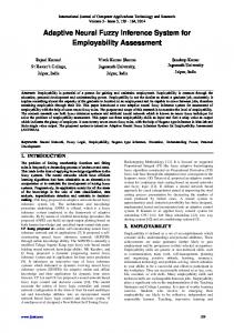
v where setting c k = 1/(number of elements in cluster k + 1) seems to work fine in practice. The total number of clusters, C, depends on these parameters. This C is the same as in equations 4.1 and 4.5, since one and only one rule per cluster is created. The clusterization algorithm is detailed in the figure below:

25

Figure 1: Clusterization Algorithm Flowchart The algorithm is similar to the Learning Vector Quantization (LQV) method [Bezd95]. The result of this algorithm is a set of crisp clusters.

26

4.3.2 Fuzzy clusterization

The Fuzzy C-means algorithm [Bezd81] is then applied as a first optimization of the clusters. The objective is to lower the value of J, where J is defined as: N C v v J = ∑∑ (u i ,k ) m xi − c k

2

(4.8)

i =1 k =1

v The number u i ,k represents the degree of membership of x i in cluster k. m is used to help to control the “fuzziness” in the clusters, if m is large so is the fuzziness and vice versa. Applying the following equations, in an alternating fashion, performs optimization of the system, i.e. the reduction of the value of J:

u i ,k

⎛ C ⎛ ⎜ = ⎜∑⎜ ⎜ ⎜ j =1 ⎝ ⎝

v v 2 ( m −1) ⎞ ⎟ xi − c k ⎞⎟ ⎟ v v ⎟ xi − c j ⎠ ⎟ ⎠

−1

⎛ N v ⎞ ⎜ ∑ (ui ,k ) m xk ⎟ v ⎠ ci = ⎝ i =1N ⎛ ⎞ ⎜ ∑ (ui ,k ) m ⎟ ⎝ i =1 ⎠

(4.9)

(4.10)

This process is repeated until J stabilizes at a value and no further improvement is expected. Once the fuzzy clusters have been created and optimized, they can be converted into rules. The following three parameters are determined for each of the C rules: mk , j = ck , j for 1 ≤ j ≤ n

27

(4.11)

σ k, j

⎛ N ⎞ ⎜ ∑ u i , k ( xi , j − c k , j ) 2 ⎟ ⎟ = ⎜ i =1 N ⎜ ⎟ u ⎜ ⎟ ∑ i ,k i =1 ⎝ ⎠

1

2

bk = c k ,n+1 , 1 ≤ k ≤ C

(4.12)

(4.13)

Since these three values are all that is needed to define the FINN, the initialization process is concluded. A popular way to store the parameters of the FINN is by using two matrices, Μ and Σ , v

and a vector b . The rows of the matrices represent the rules that compose the systems. Μ conv

tains the values of the μ ’s, while Σ and b store the values of the σ ’s and the b’s, respectively. For example, element (1,2) of Μ is the value for μ1,2 . Similarly, the 4th element of the vector v b would be b4 .

4.3.3 Optimization

Notice that the result expressed in equation 4.5 is differentiable with respect to any of the defining parameters of the FINN in question. Hence, the MSE defined in equation 3.5. is also differentiable, with respect to the parameters. This is true although the function f in equation 3.5 would, in this case, represent a FINN, and not an ANN. Actually, using equations 4.2, 4.4, and v 4.5, it can be proven that for a given input vector x i :

v ∂ ( f (x i ) − yi ) 2 v = ( f (x i ) − yi ) ∂ bh

v fs h ( x i ) C v ∑ fs k (x i ) k =1

28

(4.14)

v v ∂ ( f (x i ) − y i ) 2 ( xi , j − mh , j )(bh − f (x i )) v ( f (x i ) − yi ) = 2 ∂mh , j σ h, j

v fs h (x i ) C v ∑ fs k (x i )

(4.15)

k =1

v v 2 ∂ ( f (x i ) − y i ) 2 ( xi , j − mh , j ) (bh − f (x i )) v ( f (x i ) − y i ) = 3 ∂σ h , j σ h, j

v fs h (x i ) (4.16) C v ∑ fs k (x i ) k =1

The derivative of the MSE, with respect to any of the parameters, can be easily obtained by repeating and adding the results obtained from the equations stated above for each of the records in the training set. These gradients can be used to implement a back-propagation algorithm designed for the FINN. The values of the gradients are not used directly to modify the values of the parameters. Instead, they are first multiplied by a positive real number called learning rate, and then are used to modify the value of the parameter by subtracting the value of the multiplication from the value of the parameter. When all the parameters of the FINN are modified, this marks the end of one cycle, called an epoch. Usually several epochs are needed before obtaining a FINN that is able to produce an acceptable MSE. This algorithm is the last optimization step for the FINN mentioned in [Rutk00].

29

4.3.4 The Tipping Example

This example can be found in the MatLab Fuzzy Logic Toolbox. It is a basic description of a two-input, one-output tipping problem (based on restaurant tipping practices in the U.S.). The system is given two numbers between 0 and 10 that represent the quality of service at a restaurant (where 10 is excellent), and the quality of the food at that restaurant (again, 10 is excellent). The system, based on these two inputs, determines what the tip should be. The example includes the exact description of this fuzzy system, i.e. shape and parameter values of all the membership functions used. The system has three rules: 1. If the service is poor or the food is rancid, then tip is cheap. 2. If the service is good, then tip is average. 3. If the service is excellent or the food is delicious, then tip is generous.

It is assumed that an average tip is 15%, a generous tip is 25%, and a cheap tip is 5%. Besides the description of the FIS, an executable version, able to produce the correct tip given the values for the quality of the food and the quality of the service, is provided. Using this version, a training set with 255 examples is created. The test set consists of 45 examples. The data can be found in Appendix 1. By setting the parameters for the algorithm detailed in section 4.3.2, four clusters are created. Specifically, the parameter values are to D = 8.0 and B = 4.0 The learning rates for the optimization algorithm of section 4.3.3 are: 0.30 for the b’s, 0.003 for the μ ’s and 0.001 for the

σ ’s. A total of 300 epochs are performed.

30

⎡4.56 ⎢4.96 The system obtained at the end of the process is: Μ = ⎢ ⎢ .64 ⎢ ⎣8.23

⎡ 2.35 ⎢ 2.27 Σ=⎢ ⎢ 3.21 ⎢ ⎣3.04

6.81⎤ 2.45⎥⎥ and 3.06 ⎥ ⎥ 6.65⎦

2.64 ⎤ ⎡15 . 92 ⎤ ⎥ 3.15 ⎥ v ⎢11 .45 ⎥ ⎥ . The graphic representation of this system can be and a vector b = ⎢ 2.77 ⎥ ⎢ 6 .55 ⎥ ⎥ ⎥ ⎢ 2.69 ⎦ ⎣ 22 .80 ⎦

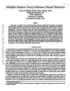
seen in Figure 2. The C program that creates the systems is shown in Appendix 2, while the MatLab program that uses the system to create the figure is in Appendix 3.

Figure 2.- Graphic representation of the Tipping Problem resulting clusters.

The projection of the clusters makes their interpretation easier. Although the rules that may be inferred from the clusters are subjective, my interpretations are: 31

Magenta Cluster: If the service is poor and the food is rancid, then tip is cheap. Green and Red Clusters: If the service is good and the food is good, then tip is average. Blue Cluster: If the service is excellent and the food is good, then tip is generous.

The rules are not the exact the rules of the original system, but they express the same idea, the better the food and/or the service, the better the tip.

32

CHAPTER 5

CREATION AND OPTIMIZATION OF FINN “Without data, all you are is just another person with an opinion.” -- Unknown

5.1

INTRODUCTION TO THE CREATION AND OPTIMIZATION OF FINN

FINNs have been successfully applied to difficult problems such as the nonlinear ball and beam system [Wang92], control problems [Seng99], angiographic disease [Rutk00] and respiratory dynamics [Babu00]. The systems have not only been able to produce small errors in the training and test set, but also create a system which can be interpreted. Although there is no expert commentary on whether the rules extracted from the trained FINN make sense, the results in the existing literature are enough to justify the search for new ways to optimize the networks. The purpose of this document is to present a new genetic algorithm for the improvement of the FINN. Contrary to the entire existing research on GAs for FINNs [Lee03, Seng99], this new algorithm considers the parameters of the network to be linked, i.e. not independent of each other. The reason is that the groups of parameters that compose a rule are intimately related, since they, as a group, describe a cluster in a multidimensional space. These ideas are explained in section 5.3. Before presenting an algorithm to improve the FINN, it is important to answer the question: is it possible to improve a FINN to a specific accuracy? After all, if under the most favorable conditions, it is possible to obtain a small squared error, then there exists the possibility of creating a FINN under more adverse conditions. There exists proof that FINNs are universal approximators [Wang92], i.e. they can approximate an objective function to any accuracy. This proof has two major disadvantages, the first being the assumption that the objective function will 33

be available, when in reality only a training and test set are available, and the second is that it is not a constructive proof. Both of these disadvantages are overcome in new proof presented in section 5.2. 5.2

ARBITRARY ACCURACY FOR A GIVEN TRAINING SET: A CONSTRUC-

TIVE PROOF 5.2.1 Basic Idea

It has been proven that FINNs are universal approximators [Wang92]. The universal approximation property, however, requires an objective function. This translates to a scenario not typically found during the solution of practical problems. Most of the time, the objective function is not available. Actually a training set, with sample points of the objective function, is what is typically available. The following is a proof that, for a given training set and a given MSE, ε > 0 , there exists a FINN with MSE < ε . 5.2.2 Sufficient Conditions

A couple of definitions should be stated: Definition 1:

Let

{

d y = max y i − y j : i ≠ j

}

(5.1)

}

(5.2)

Definition 2:

Let

{

v v d x = min x i − x j

34

2

:i ≠ j

where • is defined as the square of the Euclidian distance between the inputs of examples. The accuracy of the FINN for the training set is measured by the mean squares error that is produced:

ε FINN =

1 N

N

∑ ( yˆ i =1

i

− yi ) 2

(5.3)

Theorem 1:

v For any training set (X, y ) with the characteristics described in Section 2, and any mean square error ε d > 0 , the FINN with the 4 characteristics described below will produce a

ε FINN < ε d . 1)

The FINN will have N rules, i.e. set M=N.

2)

Set μi , j = x i , j , ∀i, j ,1 ≤ i ≤ N ,1 ≤ j ≤ n .

3)

Set σ i2, j = σ ≤

4)

Set bi = yi , ∀i,1 ≤ i ≤ N .

− dx ⎛ εd ln⎜ ⎜ ( N − 1)d y ⎝

⎞ ⎟ ⎟ ⎠

, ∀i, j ,1 ≤ i ≤ N ,1 ≤ j ≤ n .

Notice that the right side of condition 3) is a positive number, since the denominator is the natural logarithm of a number which is less or equal than 1. The proof is shown in 2 parts. In Part1 it is demonstrated that N v v ∀x ∈ X, d y ∑ fs k (x) ≤ ε d ⇒ ε FINN < ε d . k =1 k ≠1

Part 2 states that if a system is constructed with Characteristics 1)-4) then

35

(5.4)

N v v ∀x ∈ X, d y ∑ fs k (x l ) ≤ ε d .

(5.5)

∀i,1 ≤ i ≤ N : ( yˆ i − y i ) 2 ≤ ε d

(5.6)

k =1 k ≠1

Proof of Theorem 1: Part 1:

Notice that if we assume that

then ε FINN ≤ ε d . Hence, proving Eq. (5.6) is equivalent to proving Eq. (5.4). Using Eq.(4.5), it can be shown that Eq. (5.6) is equivalent to: N v ∑ bk fsk (x i )

k =1 N

v ∑ fsk (x i )

− yi ≤ ε d , ∀i,1 ≤ i ≤ N

k =1

r Notice that for any particular input vector xl , by C.2 and C.3: N v v bl fsl (x l ) + ∑ bk fsk (x l )

N

v ∑ bk fsk (x l )

k =1 N

v ∑ fsk (x l )

k =1 k ≠l N

− yl =

v v fsl (x l ) + ∑ fsk (x l )

k =1

− yl

k =1 k ≠l

N v yl + ∑ bk fsk (x l )

=

k =1 k ≠l N

v 1 + ∑ fsk (x l )

− yl

k =1 k ≠l

N N v v yl + ∑ bk fsk (x l ) − yl − yl ∑ fsk (x l )

=

k =1 k ≠l

k =1 k ≠l

N v 1 + ∑ fsk (x l ) k =1 k ≠l

36

(5.7)

N N v v ∑ bk fsk (x l ) − yl ∑ fsk (x l )

=

k =1 k ≠l

k =1 k ≠l

N v 1 + ∑ fsk (x l ) k =1 k ≠l

N

v − yl ) fsk (xl )

∑ (b =

k =1 k ≠l

k

N

1+ ∑ k =1 k ≠l

(5.8)

v fsk (xl )

Notice that the final term in Eq. (5.8) will be at its maximum when the denominator is minimum. By Eq. (4.2) and Eq.(4.4): v 0 < fsk (x i ) ≤ 1, ∀k , i,1 ≤ k , i ≤ N

(5.9)

Therefore: N

∑ (b k =1 k ≠l

k

v − y l ) fs k (x l ) N

1+ ∑ k =1 k ≠l