Cross-Guided Clustering: Transfer of Relevant Supervision across Domains for Improved Clustering Indrajit Bhattacharya, Shantanu Godbole, Sachindra Joshi and Ashish Verma
[email protected],
[email protected],
[email protected],
[email protected] IBM Research, India
Abstract—Lack of supervision in clustering algorithms often leads to clusters that are not useful or interesting to human reviewers. We investigate if supervision can be automatically transferred to a clustering task in a target domain, by providing a relevant supervised partitioning of a dataset from a different source domain. The target clustering is made more meaningful for the human user by trading off intrinsic clustering goodness on the target dataset for alignment with relevant supervised partitions in the source dataset, wherever possible. We propose a cross-guided clustering algorithm that builds on traditional k-means by aligning the target clusters with source partitions. The alignment process makes use of a cross-domain similarity measure that discovers hidden relationships across domains with potentially different vocabularies. Using multiple realworld datasets, we show that our approach improves clustering accuracy significantly over traditional k-means. Keywords-Clustering methods; Transfer Learning; Relationship Discovery;
I. I NTRODUCTION Clustering is a critical tool for data exploration, and owes its popularity to its unsupervised nature. Clustering variations use different similarity measures and intrinsic goodness measures to group ‘similar’ data items together [1]. However, maximizing intrinsic goodness often does not correlate well with human notions of interestingness or usefulness. This happens largely because such notions are often hard to capture in terms of unsupervised similarity measures over representations of the data items. Thus, the same absence of supervision that makes clustering popular, also leads to challenges in interpreting its outcome. Obtaining supervision, as the alternative, requires expertise and significant effort from human supervisors. In this paper, we investigate if supervision can be reused or transferred from previous tasks to guide a new clustering task. In the new setting, a clustering algorithm is provided with a set of data items and a similarity measure from a target domain. Additionally, it has access to a data-set from a different domain, which we call the source domain, along with a supervised partitioning of the source data items. This partitioning may have been manually created, as for training data in the classification setting, or may be a manually reviewed and refined version of a clustering output. We will assume that target clusters that are ‘similar’ to the source partitions are more useful to the human
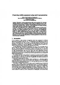
user. To be able to use this source supervision, the target clusters need to be ‘aligned’ with relevant source partitions. Note that this alignment unavoidably comes at the cost of clustering goodness, as defined solely in terms of the target similarity measure. If no relevant source partitions are found, clustering using the target similarity measure remains the fall-back option. This problem is an instance of transfer learning [2]. This variant, where unsupervised learning needs to be performed in the target domain given supervision in the source domain, has not received much attention in the literature. In practice, such relevant supervision is often readily available. Lawyers involved in corporate legal audit routinely need to group and categorize emails and other documents for different corporate cases. They can benefit significantly if categories created in one case can be used to guide another. As another example, consider a service desk, where quality analysts need to group customer survey comments in different corporate accounts. Figure 1 shows some illustrative phrases from surveys for an automobile company, which is the target domain. Clustering based only on target data yields clusters corresponding to Agents, Parts and Accessories, and Servicing (Fig 1(a)). However, these may not be the clusters that the analyst desires. Instead, if he wanted clusters around Personnel and Car-related issues, he could provide a survey collection from a related account as the source collection, where he has already created supervised partitions around Motor Cycles Issues and Sales Personnel (Fig 1(b)). This leads to deviation from the original target clusters to align with the source partitions. Note that this deviation should be less when the source partitions are less ‘relevant’. For example, the desired Car-related cluster would not emerge as clearly had the analyst provided a source collection partitioned around Computer Parts and IT Technicians. Alternatively, if the desired clustering is around customer sentiments, a different source collection that is partitioned around sentiments could be provided. Fig 1(c) shows the result of providing such supervision from a telecommunication domain, which is very different from the target automobile domain, apart from the sentiment-related concepts. Observe that the desired number of clusters in the target need not be the same as the number of partitions in the source domain. ‘Irrelevant’ partitions from the source, e.g. a partition
Figure 1.
Example of different sources influencing target clustering. Rectangles represent source partitions and ovals represent target clusters.
around Signal Quality issues, should not influence the target clustering. Also, target concepts that are unrelated to any source partition (‘Car Parts’ in Fig 1(c)) should be clustered purely based on the target similarity measure. In this paper, we propose a novel framework that aims to strike a balance between clustering goodness on a target domain and alignment with a relevant supervised partitioning of a source collection. For this, we present a cross-guided clustering algorithm that uses conceptual similarities across domains to guide the traditional k-means paradigm. A crucial aspect is measuring similarity of clusters across domains where the correspondences between the data attributes or vocabularies is not known. To discover and measure hidden relationships across domains, we propose a cross-domain similarity measure based on pivot words across vocabularies. We demonstrate using multiple real-world text datasets that cross-guided clustering improves clustering accuracy significantly over traditional k-means by transferring supervision from a related domain. The rest of our paper is organized as follows. We first review our problem in the light of related work in Section II. Then we formalize our problem and motivate the crossguided clustering framework in Section III. In Section IV and Section V, we present our clustering algorithm and the cross domain similarity measure. In Section VI, we present an analysis of favorable and unfavorable conditions for cross-guided clustering and propose a quantitative measure for cross-domain ‘clusterability’. Finally, we present experimental results in Section VII and conclude in Section VIII. II. R ELATED W ORK In this section, we review our work in the light of related research from the areas of clustering and transfer learning. Semi supervised clustering aims to improve clustering performance by limited supervision in the form of a small set of labeled instances. Wagstaff et. al. [3] provide labeled data in the form of pair-wise must-link and cannot-link constraints among data instances. The original clustering criterion is modified to additionally minimize the number of constraint violations. Basu et al. [4] use labeled data to generate initial seed clusters as well as use constraints generated from labeled data to guide the clustering process.
Alternatively, a small set of labeled instances can be used to learn a parameterized distance function [5], [6]. The coclustering approach [7], [8] clusters related dimensions simultaneously through explicitly provided relations between them, such as words and documents, or people and reviews. Bhattacharya and Getoor [9] use a combination of attributebased and relational similarity for collective clustering over observed relationships among the data items. In contrast, in our work in this paper supervision is discovered in the form of cluster level similarities obtained from labeled instances from a different domain, having different but related labels. Our work is closely related to the area of transfer learning [2]. Several methods aim to improve the accuracy of a supervised classifier by learning from labeled data from a different domain [10], [11], [12], [13], [14]. For example, Blitzer et.al. [13] investigate domain adaptation for supervised sentiment classification using pivot features to link the source and target domain. The pivot features are chosen by selecting frequently occurring common words that have high mutual information with class labels in the source domain. Dai et al. [14] propose a transfer learning algorithm for text classification using an EM-based naive Bayes classifier. In the context of unsupervised transfer learning, Dai et al. [15] propose self-taught clustering to cluster a small collection of unlabeled data in a target domain by using a large amount of auxiliary unlabeled data in a source domain. They propose a co-clustering-based method that simultaneously clusters target and auxiliary data where the source clustering influences target clustering through a common set of features. Unlike all these methods, we focus on improving clustering performance in a target domain using labeled data from a different, but potentially related source domain, where the relations across domains are hidden and measuring them is non-trivial. III. P ROBLEM F ORMULATION As in a standard clustering problem, we are given a set of data items {t1 , t2 , . . . , tn }. We call the domain of this data the target domain T . Our goal is to partition the data items into k target clusters {C1t , C2t , . . . , Ckt }. We consider a hard clustering setting, where each of the target data items ti is assigned to exactly one cluster Cjt . In the k-means setting,
the partitioning of the data items is done based on nearness to one of k centroids {C¯it }, based on a given distance measure dt (tj , C¯it ) between a data item and a centroid in the target domain. The divergence Dt (Cit ) of any cluster Cit is the summed squared distance of each data item in that cluster from the corresponding ‘centroid’ C¯it : X Dt (Cit ) = (dt (tj , C¯it ))2 δ t (tj , Cit ) tj
where δ t (tj , C¯it ) is 1 if item tj is assigned to cluster Cit and 0 otherwise. The standard goal of k-means clustering is to P findt thet k best centroids for which the total divergence i D (Ci ) over all clusters in the target domain is minimized. In our new setting, we are additionally given a different set of items {s1 , s2 , . . . , sm }, possibly from a different domain S, which we call the source, and an assignment of those items to k 0 source partitions {C1s , C2s , . . . , Cks0 }. For each source partition, we also have a source centroid C¯js . For notational convenience, in the rest of the paper, we use the superscripts s, t and x to indicate source, target and cross domain, respectively. We would like to align the target clusters with the source partitions to guide the target clustering. However, the source and target domains may be different. In other words, the vocabulary V s of the source — the attributes over which the data items and centroids are defined — may be different from the target vocabulary V t . As a result, the distance measure dt (), which assumes the same vocabulary for the compared items or centroids, may not apply across domains. In such cases, a different cross-domain distance measure dx (ti , sj ) is needed to compare clusters across domains. For now, we assume that dx () is also provided to us. In Section V, we will discuss how such a measure may be defined. Just as the target distance measure dt () is used to assign target data items to target centroids and measure target divergence, the cross domain distance measure dx () is used to align the target centroids with the source centroids and measure cross domain divergence. However, the nature of the cross domain alignment is different from that of target items to target centroids — each target cluster should be aligned with at most one source partition, and vice versa. In our example, source S1 has one ‘Personnel’ partition, so we would want all target documents similar to ‘Personnel’ documents to be grouped into a single target cluster. Also, if the source has a separate ‘Car related’ partition, the target ideally should not have a single cluster related to both ‘Car’ and ‘Personnel’. Given such a cross-domain alignment between source partitions and target clusters, we measure the cross domain divergence as XX Dx (C t , C s ) = (dx (C¯it , C¯js ))2 δ x (Cit , Cjs )|Cit | (1) Cit Cjs
where δ x (Cit , Cjs ) is 1 if Cit is aligned with Cjs , and 0 otherwise. Observe that weighting by the size |Cit | of each cluster Cit is needed to make Dx (C t , C s ) comparable to Dt (Cit ), which is obtained by summing over the distance of each data item in Cit from its centroid. Assigning items to centroids in the target is simple given dt (). But finding a cross domain alignment is more complex. We construct a bipartite cross domain graph Gx that has one set of vertices S corresponding to source centroids, and another set T corresponding to target centroids. We add an edge between every pair of vertices (i, j) from S and T where the weight of the edge is given by 1 − dx (C¯it , C¯jt ). Then finding the best alignment is equivalent to finding the maximum weighted bipartite match in the graph Gx . Recall that a match is a subset of the edges such that any vertex is spanned by at most one edge, and the score of a match is the sum of the weights of the included edges. The only issue with defining the cross domain alignment as the best match in Gx is that it is a complete bipartite graph. So, the maximum match forces every target cluster to be aligned with one source partition (given enough source partitions), however dissimilar any target cluster may be with the source. One solution may be to disregard all edges in the match with weights below some threshold. Alternatively, we modify the definition of δ x (C¯it , C¯js ) for Dx () to be the match weight if Cit is aligned with Cjs , and 0 otherwise. With this modified definition, weaker the match with the source, the lower is the penalty for divergence from that source centroid. For the ‘Car’ cluster in our example from the introduction, penalty for divergence from the ‘Bike’ partition is higher than that from a ‘Computer’ partition. Given k target centroids, an assignment of target items to these centroids, and an alignment between source partitions and target centroids, the combined divergence measure looks to strike a balance between target divergence and cross domain divergence: D(C t , C s ) = αDt (C t ) + (1 − α)Dx (C t , C s )
(2)
where α captures the relative importance of the two divergences over all clusters. Observe that α=1 corresponds to target-only clustering, while α=0 leads to target clusters that are as similar as possible to source partitions, but not tight internally. In the cross clustering problem, the goal, given a source partitioning C s , is to find k centroids in the target that minimize the combined divergence D(C t , C s ). In the next section, we present an iterative algorithm that minimizes this combined divergence. IV. C ROSS -G UIDED C LUSTERING A LGORITHM Our algorithm for minimizing the objective function in Equation (2) starts from an initial set of k target centroids and then proceeds by iteratively reducing the divergence by an alternating optimization approach. This is similar in spirit to the traditional k-means algorithm, that executes two steps
in every iteration — first assign items to existing centroids, and then reduce divergence by re-estimating the centroids based on the current assignment of items. Our cross-domain divergence depends both on the current centroids and the cross domain alignment. As a result, we go over one additional step in every iteration — first a) update the item assignment based on the current centroids, then b) update the cross-domain alignment based on the current centroids, and finally c) minimize divergence by re-estimating the centroids based on the current item assignment and the current crossdomain alignment. Updating the item assignment is straight forward — each item gets assigned to its nearest centroid according to the target distance measure dt (). For updating the crossdomain alignment, we find the maximum weighted bipartite matching between the source and target centroids, using the popular ‘Hungarian algorithm’ [16]. Re-estimating the target centroids to minimize divergence depends on the target data items, as well as the source centroids. To find the re-estimation rule, we need to differentiate the divergence function with respect to the target centroids. Our divergence function is carefully designed to ensure differentiability with respect to target centroids. On t ,C s )) = 0, we differentiating and explicitly solving d(D(C d(C¯it ) th t ¯ obtain the update rule for the i centroid Ci to be P P α ti ∈C t ti + (1 − α) j δ x (Cit , Cjs )C¯js i P C¯it = (3) α|Cit | + (1 − α)|Cit | j δ x (Cit , Cjs ) The intuitive interpretation of the update rule is as follows. As in traditional k-means, each centroid tries to move to the ‘center’ of the items currently assigned to it. This is reflected in the first term of the numerator. The other movement in the cross-domain setting is toward its matched centroid from the source. This is captured by the second term in the numerator. However, this movement is dampened by the extent of match with the source centroid — a target centroid that does not have a significant match in the source domain is not affected by the source at all. Observe that this is one significant difference with movement in the target domain. All target data items are assumed to correspond to some target centroid — in contrast, a target centroid may not have a corresponding source centroid. Also, the two movements are traded off by the parameter α, which can be thought of as a ‘prior’ on the relevance of the source and the target over all clusters. The high-level cross-guided clustering algorithm is described in Figure 2. The algorithm creates the source centroids in step 3, and initializes the target centroids in steps 5-8. Initialization is a challenge even in the traditional kmeans algorithm, since the algorithm is prone to getting caught in local minima. The challenge becomes more significant for cross-guided k-means because of the cross-domain alignment step involved. Until the initial clusters achieve
Algo CrossGuidedCluster Params: Doc Sets Dt , Ds , Partitioning C s on Ds , Int k 1. 2.
Establish pivot vocabulary between source and target Create projection matrix for each vocabulary
3. 4.
Compute source centroids C s Project each source centroid to pivot vocabulary
5. 6. 7. 8.
% Initialize target clusters Initialize k centroids Iterate n times or until convergence Assign each document in Dt to nearest centroid Recompute k centroids from assigned documents
% Start cross-guided k-means 9. Iterate m times or until convergence 10. Project each target centroid onto pivot vocabulary 11. Create cross domain similarity graph Gx over C s and C t 12. Compute maximum bipartite matching over Gx 13. Iterate over k target centroids C t 14. Update centroid using cross domain rule 15. Assign each document in Dt to nearest centroid 16. Return k target centroids Figure 2.
Cross-Guided Clustering algorithm
low divergence, no significant match can be discovered with the corresponding source centroid using the cross domain similarity measure. On the other hand, if the divergence of the initial target clusters reach their minima before they are aligned with the source centroids, the target clusters may settle down to a specific facet of the target domain, which again may not be similar to the source partitioning. In view of this, in the initial step, the algorithm executes a few iterations of k-means, which are enough for patterns to emerge in the target clusters, but do not allow the clusters to settle down. Each cross-guided k-means iteration is shown in steps 10-15. The cross domain similarity computation involves establishing a pivot vocabulary between domains (steps 1-2) and projecting the centroids on the pivot vocabulary. The projection needs to be done only once for the source centroids (step 4), but needs to be repeated for every target centroid after every re-estimation step (step 10). We elaborate on these steps in the next section. V. C ROSS D OMAIN S IMILARITY The success of the cross-guided clustering approach often depends on the design of the cross-domain distance measure dx (Cit , Cjs ) between a target and a source centroid, since the source and target centroids are from different datasets. Typically, for documents, distance is defined as d( Cit , Cjs ) = 1 − cosine(Cit , Cjs ), where cosine(v1 , v2 )
captures the cosine similarity of two weight vectors: X cosine(v1 , v2 ) = wt(v1 , ai ) × wt(v2 , ai ) ai
where ai ’s are the dimensions of the two vectors. When comparing two centroid vectors, this compares weights over words that are lexically the same. However, two different problems arise when the centroids are from two datasets from different domains having different vocabularies. First, words that are lexically the same may not have the same meaning in two domains. Secondly, the two domains may have synonyms that are not lexically similar, which will be ignored in the above similarity computation. This is a challenging problem in itself and has been the focus of some research [13]. In this section, we discuss how similarity measures can be adapted to handle these two problems. Pivot Vocabulary We first address the problem of lexically identical words not being semantically identical in the two domains. We construct the pivot vocabulary V p , consisting of the words from the two vocabularies that are lexically identical. For each word v in the pivot vocabulary, we construct their pivot weights pw(v) that captures its semantic similarity in the two domains as follows. To compute pw(v), we assume that a word is semantically similar across the two domains if it is used in similar contexts. For both the source and target domains, we construct the word-word context matrix Cxt. Cxt(v, v 0 ) counts the number of times words v and v 0 occur within m tokens of each other over all documents in the domain. We use standard TF-IDF weighting to assign a weight to each entry in the context matrix. The context vector Cxt(v) for any word v is the row corresponding to v in the matrix Cxt, and captures the aggregated context of v in the particular domain. The pivot weight pw(v) is then calculated as the cosine similarity of its two context vectors, Cxts (v) from source and Cxtt (v) from target: pw(v) = β + (1 − β)cosine(Cxts (v), Cxtt (v)) where β provides smoothing over sparsity and noise in the data. The similarity between a source and target centroid can now be computed using a modified version of cosine similarity that takes the pivot weights into account: X simx (C¯it , C¯js ) = wt(v, C¯it ) wt(v, C¯js ) pw(v) v∈V p
where wt(v, C¯it ) captures the weight of pivot word v in the ith target centroid C¯it . Projection onto Pivot Vocabulary The other problem with comparing centroid vectors over different vocabularies is that words not in the shared vocabulary are completely ignored. For example, if a context center agent is referred to an ‘agent’ in one domain, and as a ‘rep’ in another, these do not contribute to any cosine similarity computation. To
address this, we take a projection approach, where weights of non-pivot words (word not in V p ), instead of being lost, are distributed over the weights of relevant pivot words. To achieve this, we construct a projection matrix P roj(v, v 0 ) for each domain from the context matrix Cxt, such that the columns correspond to pivot words from V p and rows correspond non-pivot words. For any non pivot word v, P roj(v, v p ) defines how its weight is distributed over pivot word v p . The projected weight wtp (v, C¯it ) for pivot word v in target centroid C¯it is the augmented weight after projecting on v weights of all relevant non pivot words in the target vocabulary V t : X wtp (v, C¯it ) = wt(v, C¯it ) + P roj t (v 0 , v) v 0 ∈V t −V p
The projected pivot weights can similarly be computed for the source domain using its own projection matrix P roj s . Cross-domain similarity of centroids is then computed using projected weights of pivot words in the two domains. VI. A NALYSIS OF C ROSS - GUIDED C LUSTERING In this section we present an analysis of cross-guided clustering, denoted as CGC for brevity. If we have the gold standard target cluster labels available, can we estimate how badly or how well cross-guided clustering will perform on that target dataset for a given source? Before heading into the experimental section, here we attempt to understand the favorable conditions for CGC and answer this question, so that we can interpret and explain the performance of CGC on various datasets. First, consider traditional k-means clustering on the target, disregarding the source. The k gold standard target centroids C¯ t are found from all the items assigned to their true clusters. Then, for each target item ti , we consider its similarity sim(ti , C¯it ) to each centroid C¯it ; i = 1 . . . k. Given these k similarities, the more unambiguously ti can be assigned to its ‘true’ centroid C¯∗t (ti ), the more easily ti is ‘clusterable’. Entropy over the k choices can be used to measure clusterability of ti . We use a simpler measure, that does not require a probability distribution, but considers how similar ti is to the nearest ‘non-true’ centroid. We define the clusterability (denoted Cab) of ti given the centroids to be Cab(ti |C t ) =
sim(ti , C¯∗t (ti )) −max{C¯jt 6=C¯∗t (ti )} sim(ti , C¯jt )
The clusterability of the entire target dataset T is obtained by averaging over the clusterability of the individual items: X Cab(T |C¯ t ) = Cab(ti |C¯ t )/|T | (4) {ti ∈T }
Note that this is an ‘upper bound’ on target clusterability using k-means, since this is conditioned on correct discovery of the target centroids. Also, the range of Cab(T |C¯ t ) is [−1.0, +1.0]. The value 1.0 is achieved for a ‘perfectly
centroid: M ab(C¯it |C¯ s ) =
simx (C¯it , C¯∗s (C¯it )) −max{C¯js 6=C¯∗s (C¯it )} sim(C¯it , C¯js )
Figure 3. clustering
(a) Favorable and (b,c) unfavorable sources for cross-guided
clusterable’ dataset, where every data item has similarity 1.0 to its true centroid, and similarity 0.0 to all other centroids. Similarly, for a ‘perfectly unclusterable’ dataset, where every data item has similarity 0.0 to its true centroid and similarity 1.0 to some other centroid, the clusterability value will be −1.0. Now consider the source centroids and their impact on cross-guided clustering. We have mentioned that a source is helpful when the target centroids C¯ t are matched by the source centroids C¯ s representing the supervised partitions. We first illustrate why imperfect matches are undesirable for CGC and then propose a measure for ‘matchability’ M ab(C¯ t , C¯ s ) of a source-target pair. In Figure 3, we illustrate different types of mappings that are possible between source and target centroids. In Figure 3(a), both target centroids are matched unambiguously by the source centroids. This is when the source is beneficial, since the source centroids provide supervision for the corresponding target centroids only, without influencing any other target centroid. Figure 3(b), illustrates the first problematic scenario. Two different target centroids are similar to the same source centroid. As a result, target data items from these two different true target clusters may gravitate toward each other and end up in the same computed target cluster. This adversely affects ‘source-side matchability’ M ab(C¯ s |C¯ t ). Similarly, Figure 3(c) illustrates the second problematic scenario. Here, a single target centroid is similar to two different source centroids. As a result, the target data items for which this is the true centroid, may be pulled away from each other end up in different computed target clusters. This adversely affects ‘target-side matchability’ M ab(C¯ t |C¯ s ). In any dataset, the overall matchability of a source-target pair is the net effect of these target-side and source-side ambiguities, and determines whether the source will be helpful for clustering the target. We now propose one possible measure for matchability. Note that other measures such as joint-entropy may also be possible to use. We first measure the matchability of a single target centroid C¯it using an approach similar to clusterability that does not require a probability distribution. We consider its cross-domain similarity simx (C¯it , C¯js ) to each source centroid C¯js , and then identify the most similar source centroid C¯∗s (C¯it ) = max{C¯js } simx (C¯it , C¯js ). This similarity is compared to that with the next closest source
The total target-side matchability is obtained by averaging over the target centroids: M ab(C¯ t |C¯ s ) = P t ¯t ¯s The source-side matchability ¯ t M ab(Ci |C )/|C |. C i s ¯t ¯ M ab(Ci |C ) of each source centroid is defined analogously by considering the difference in similarity to its closest target centroid and the next closest target centroid. The total source-side matchability M ab(C¯ s |C¯ t ) is again obtained by averaging over the all source centroids. Finally, the matchability M ab(C¯ t , C¯ t ) of a source-target pair is the average of source-side matchability and target-side matchability: M ab(C¯ t , C¯ s ) = (M ab(C¯ t |C¯ s ) + M ab(C¯ s |C¯ t ))/2 Again, this is an ‘upper bound’ on how beneficial a particular source can be for clustering a target dataset, since this is conditioned on the discovery of the true target centroids. Observe, that unlike for target clusterability, for matchability we considered the most similar source centroid for a target centroid, and vice versa, instead of the ‘true’ matching centroid. The reason is that for clusterability, it is not enough for a target data item to unambiguously select any gold standard centroid - it has to choose its ‘true’ centroid. For matchability, there is no such requirement. It is sufficient for each target centroid to match up with any source centroid unambiguously to obtain supervision for helping target clustering. One consequence of this is that matchability scores cannot be negative and lie in the range [0.0, 1.0]. Finally, the cross domain clusterability of a target dataset, given a set of source centroids, is a linear combination of clusterability of the target alone and the matchability of the source and the target, following Equation (2) and using the same trade-off parameter α: Cab(T |C s , C t ) = αCab(T |C t )+(1−α)M ab(C s , C t ) (5) Now, given a target dataset with its gold standard cluster labels, and a source partitioning, we can use Equation (4) and Equation (5) to estimate whether cross-guided clustering using this source can help result in a better clustering of the target, compared to traditional k-means clustering. They also enable us to perform controlled experiments by creating datasets with varying target clusterability and source-target matchability and evaluate how CGC actually performs under different source-target combinations. We next move on to the experimental section where we perform such experiments in a systematic way.
VII. E XPERIMENTS In this section, we present empirical results that show the effectiveness of our cross-guided clustering approach (CGC). First, we describe our datasets, and then investigate the performance of CGC over varying levels of relatedness between source and target domains and over varying parameter settings. Experimental Setup: For our experiments, we created source-target pairs from bench-mark text categorization datasets. For a target data collection with k class labels, our goal is to partition the documents into k clusters, such that clusters correspond to class labels. In other words, a pair of documents should be in the same cluster if and only if they are given the same class label by a human supervisor. Traditional methods are not expected to generate such target clusters that correspond with class labels. But, this is the clustering that a human user would create given this dataset. Accordingly, we want CGC to be able to recreate this target clustering when provided with a related partitioning (according to class labels) from a different dataset. We evaluate clustering quality by considering the correctness of clustering decisions over all document pairs. We report the standard F1 measure and Adjusted Rand Index (ARI) over the pairwise clustering decisions. The F1 measure is the harmonic mean of precision and recall over pairwise decisions. The standard Rand Index with respect to a gold standard clustering is defined as (a+b)/(a+b+c+d) where a is the number of true positive pairs, b is the number of true negative pairs, c is the number of false positive pairs and d is the number of false negative pairs. The Adjusted Rand Index improves on this by accounting for chance correlations and is defined as 2(ab − cd)/((a + d)(d + b) + (a + c)(c + b)). DataSets: We created meaningful source-target pairs from three benchmark text categorization datasets - 20 newsgroups1 (20NG), Reuters Corpus Volume 1-v2 (RCV1)[17] and Dmoz from the TechTC repository2 [18]. We have made the actual processed datasets and their descriptions available online3 . Here we briefly summarize their creation process and content. For each dataset, using domain knowledge, we first grouped the available categories (with sufficient number of documents) according to semantic or topical closeness. Then we created the source and target datasets by picking groups with at least two categories and then randomly selecting one category from the group for the source and another for the target. For all categories selected for a source or target dataset, we included all documents from those categories to the dataset. We created the first dataset from 20NG. We chose 5 categories, namely graphics, autos, sci.crypt, politics.misc, 1 http://people.csail.mit.edu/jrennie/20Newsgroups/ 2 http://techtc.cs.technion.ac.il/ 3 http://www.ibhattacharya.net/DATA/cgc.html
and religion.misc for the target collection (5000 documents), and corresponding classes xwindows, motorcycles, electronics, politics.mideast and atheism for the source (5000 documents). For RCV1, of the three available facets, we used Industries (RCV1Ind) and Topics (RCV1Top). We did not find enough meaningful category groups for the Regions facet. For RCV1Top, we included 5 categories legal proc, external markets and exports, inf lation prices and price indices, weather conditions and all matters relating to religion in the target
(991
documents)
and
5
corresponding
categories
criminal law, domestic markets sales and imports, levels of personal spending income and debt, pollution, and people in the news prof iles politicians in the source
(1702 documents). We created a source-target combination in similar way for RCV1Ind with a total of 12 categories in both source (1336 documents) and target (1076 documents). For Dmoz, since a hierarchical organization of the categories is available, we picked 14 high-level categories and selected two categories from the subtree of each of those, and added one to the source and the other to the target. For example, we added Arts/M usic/Styles By Decade/1980s to our source and Arts/M usic/Bands and Artists/U to the target from the Arts category. We ended up with 1533 documents in the target and 1384 in the source. We pre-processed all documents in a standard way using word stemming, and pruning stop-words and infrequent words (occurring less than 5 times in the dataset). Baselines: As the first baseline, we have the traditional k-means algorithm (KM) that considers only the target dataset for clustering it. Since this baseline is unaware of the source documents, we compare with a second baseline (KM-ASD) that (A)dds all the (S)ource (D)ocuments to the target and then performs traditional k-means for clustering them. However, we evaluate this by considering the pairwise decisions only over documents from the target dataset — the source documents are ignored for evaluation. Since clustering quality for both baseline k-means and CGC depends on initial centroids, in each experimental run, the compared algorithms were seeded with the same initial centroids. All reported performances are averages over 30 runs with random initializations. As our default parameter values, we set α = 0.5, initial number of target k-means iterations to 5, and maximum number of iterations to 25. Also, we set the number of clusters for both baselines and CGC as the actual number of target clusters in the data. CGC vs Baselines: In our first experiment, we compare CGC with default parameters against KM and KM-ASD. The results are plotted in Table I. We include the clusterability(Cab) values for all datasets both for k-means and CGC as a confirmation that the intuitive relatedness of the source and target clusters is actually validated by the data,
20NG Dmoz RCV1Top RCV1Ind
KM 0.054 0.127 0.158 0.114
Clusterability KM-ASD 0.056 0.131 0.166 0.116
CGC 0.129 0.200 0.294 0.212
KM 0.443 0.419 0.507 0.205
F1 KM-ASD 0.408 0.416 0.514 0.221
CGC 0.501 0.476 0.756 0.362
KM 0.292 0.368 0.359 0.120
ARI KM-ASD 0.251 0.364 0.353 0.137
CGC 0.373 0.433 0.669 0.299
Table I C OMPARISON OF KM, KM-ASD AND CGC OVER 4 DATASETS USING C LUSTERABILITY, F1 AND ARI.
and that CGC is expected to improve target clustering for these datasets. We can see that CGC significantly improves performance over both baselines in all four datasets according to both F1 and ARI measures. The CGC improvements are statistically significant in all cases over 30 runs with 99% confidence using the paired t-test. Noticeably, the Cab measure is generally able to mirror the actual performances. The actual gains using CGC in terms of F1 and ARI are greater when estimated gains according to Cab are higher. The improvement over KM proves that CGC is able to automatically discover relevant supervision from the source to improve target clustering. The improvement over KM-ASD confirms that the improvement is due to the supervision (the cluster/partition labels) available in the source, and not the source documents themselves. Notice that KM-ASD shows a small improvement over KM for RCV1Ind suggesting that more documents can help sometimes. However, on the other hand, performance of KM-ASD drops below that of KM for other datasets. For the rest of our experiments, we only report clusterability(Cab) and F1 for KM and CGC. The results for KM-ASD and with ARI have similar trends. Varying α: Recall that CGC involves a parameter α that trades off target divergence with cross-domain divergence. In all experiments so far, α was held fixed at 0.5. Next, we investigate the effect of α on CGC. In Figure 4(a) and (b), we plot CGC performance using F1 and Cab (average of 30 runs) against KM over varying α for the RCV1Ind and 20NG datasets respectively. Expectedly, CGC is identical to baseline k-means at α = 1.0. CGC performance improves with decreasing α until a threshold (0.5 for RCV1Ind and 0.6 for 20NG) and then tapers off once maximal benefit has been extracted from the source. Varying Relevance of Source: In the first experiment, each target cluster was provided with a corresponding partition in the source. In our next experiment, we investigate how performance of CGC changes when provided with a less relevant source and different numbers of source partitions. In the following, we use m/n to mean that m out of n partitions in the source are relevant for the target. Keeping 4 20NG categories in the target (religion, graphics, autos, hockey ), we start with the most relevant source (4/4) containing 4 relevant categories (atheism, xwindows,
(a)
(b) Figure 4.
Perf. vs α for (a) RCV1Ind and (b) 20NG
motorcycles, baseball). Then we reduce source relevance in 3
different ways. The results for all 3 are recorded in Table II. All performances are averaged over 10 runs. In the first setting, we replace the relevant source partitions one by one with one of the remaining partitions in 20NG. For example, we replace xwindows with sci.space, motorcycles with sci.med etc. We can see that, as expected, performance of CGC gradually drops as relevant source partitions are removed, since fewer target clusters are able to find relevant supervision from the source. The Cab measure also suggests similar degradation of performance. Note that in the first setting, we still provided a source which had the same number of partitions as the target. In the
Source 4/4 3/4 2/4 2/4 2/5 2/6 2/8 4/4 3/3 2/2 1/1
Clusterability F1 KM CGC KM CGC Replacing source partitions 0.072 0.283 0.637 0.824 0.072 0.215 0.653 0.735 0.072 0.201 0.626 0.706 Adding source partitions 0.072 0.201 0.626 0.706 0.072 0.185 0.623 0.685 0.072 0.170 0.650 0.681 0.072 0.151 0.628 0.692 Removing source partitions 0.072 0.283 0.637 0.824 0.072 0.275 0.626 0.724 0.072 0.257 0.602 0.644 0.072 0.285 0.620 0.620
Table II P ERF. OF KM AND CGC ON 20NG OVER VARYING RELEVANCE OF SOURCE . S TATISTICALLY SIGNIFICANT IMPROVEMENTS ARE IN BOLD .
second setting, we keep 2 related partitions in source, and gradually introduce more partitions from those remaining in 20NG, so that now the number of source partitions is more than the number of target clusters. With 2, 3, 4 and 6 new partitions added to 2 original relevant partitions, we can see that performance of CGC remains reasonably stable, as also suggested by Cab. This is reassuring since it suggests that when a host of source partitions are provided to CGC, it is able to seek out the relevant partitions in the source, disregarding the remaining ones. The small drop in performance is explained by the fact that the newly added partitions were not completely irrelevant to the true target clusters. This was revealed in the clusterability analysis. For example, it turned out that religion.misc is somewhat similar to politics.guns in addition to its intended source partition atheism, and comp.graphics has similarities to both sci.electronics and comp.hardware. These one-tomany mappings are weak, and they hurt CGC Cab to a small extent. In the third setting, we gradually remove relevant partitions from the source, so that CGC is left with fewer partitions in the source that in the target. We can see that actual performance gradually falls away expectedly as source partitions are removed and gets close to KM performance. The above experiments clearly show the ability of CGC to seek out relevant supervision when provided with a source partition with arbitrary number of partitions and improve clustering performance over traditional k-means. Note that due to different initializations, the avg KM performance is different across experiments, but the improvements using CGC (with the same initializations) are statistically significant where pointed out. A natural consequence of the above sequence of experiments is to wonder if a source can adversely affect
Figure 5.
CGC vs α and KM for RCV1IndBad
target clustering. With significant effort, and using our clusterability measure, we were able to create a source target combination (RCV1IndBad) from RCV1Ind by creating many-to-one and one-to-many correspondences between source (6 categories, 378 documents) and target (6 categories, 252 documents) datasets. For example, corresponding to T elevision and Radio in target, we added P rinting and P ublishing and N ewspaper P ublishing in source. In Figure 5, we plot CGC and KM performance using F1 versus α for RCV1IndBad. We can see that CGC performance gradually drops below that of KM as α increases. In summary, this demonstrates that it is indeed possible to misguide CGC by deliberately creating an adversarial source for a target dataset. But, in practice, a source will not be provided by an adversary, but by the same user who desires to guide a target clustering in a specific way. Pivot Weights: Finally, we evaluate the benefits that come from pivot probabilities and the projection approach. On comparing cross clustering with (CGCP) and without pivot weights (CGC), we found significant differences in terms of clusterability(Cab) for three of our four datasets. (Table III). However, there were no significant differences in terms of F1. The use of projection also did not lead to significant change in CGC performance. As an artifact of our evaluation process, our source and target datasets contain documents from the same domains, as a result of which their vocabularies are not significantly different. In settings where less words are shared across datasets and shared words also differ in usage, we expect to obtain more significant benefits using our cross-domain similarity measure. Noticeably, though the actual cross domain similarity values changed significantly from the use of pivot weights and projection on the pivot vocabulary for all datasets, the impact on clusterability was not as much. The intuition that we obtained from our experiments is that change in cross domain similarity values do not necessarily result in change in ambiguities for source-target mappings, which is what impacts clusterability.
20NG RCV1Ind RCV1Top Dmoz
KM 0.054 0.114 0.157 0.127
CGC 0.118 0.212 0.263 0.167
CGCP 0.143 0.211 0.294 0.200
Table III E FFECT OF P IVOT W EIGHTS ON C LUSTERABILITY
Summary of Experiments: To summarize, we have seen that CGC improves clustering performance over traditional k-means baselines significantly over multiple bench-mark datasets. Our controlled experiments, where we systematically change the nature and number of the source partitions, demonstrate that CGC is robust, and can selectively seek out relevant source partitions and improve benefit from them, while largely ignoring unrelated partitions. Though CGC involves a tunable parameter α, and setting α optimally remains an issue, the gains, even with its default value, are quite significant. VIII. C ONCLUSIONS AND F UTURE W ORK In this paper we have presented cross-guided clustering that transfers relevant supervision across datasets, potentially from different domains, to make clusters meaningful and useful for human users. This is achieved by trading off intrinsic goodness of clusters for alignment across domains. We have presented a cross-domain similarity measure for discovering similarity of concepts across domains with different vocabularies. Our experiments on real-world benchmark text datasets show that cross-guided clustering consistently and significantly outperforms traditional clustering over a variety of settings. In future, we will explore a richer language driven cross-domain similarity measure, and the use of multiple source domains simultaneously. ACKNOWLEDGMENT The authors would like to thank Ashwin Srinivasan for his insights and suggestions that helped significantly in improving the paper and its overall readability. R EFERENCES [1] P. Berkhin, “Survey of clustering data mining techniques,” Technical Report, Accrue Software, 2002. [2] S. Thrun and L. Pratt, Learning to learn. Kluwer Academic Publishers, 1998. [3] K. Wagstaff, C. Cardie, S. Rogers, and S. Schrodl, “Constrained k-means clustering with background knowledge,” in International Conference on Machine Learning, 2001. [4] S. Basu, A. Banerjee, and R. J. Mooney, “Semi-supervised clustering by seeding,” in International Conference on Machine Learning, 2002.
[5] M. Bilenko and R. J. Mooney, “Adaptive duplicate detection using learnable string similarity measures,” in ACM SIGKDD International Conference on Knowledge Discovery and Data Mining, 2003. [6] D. Klein, S. D. Kamvar, and C. Manning, “From instancelevel constraints to space-level constraints: Making the most of prior knowledge in data clustering,” in International Conference on Machine Learning, 2002. [7] I. Dhillon, S. Mallela, and D. S. Modha, “Informationtheoretic co-clustering,” in ACM SIGKDD International Conference on Knowledge Discovery and Data Mining, 2003. [8] N. Slonim and N. Tishby, “Document clustering using word clusters via the information bottleneck method,” in The Annual International ACM SIGIR Conference, 2000. [9] I. Bhattacharya and L. Getoor, “Collective entity resolution in relational data,” ACM Transactions on Knowledge Discovery from Data, vol. 1, no. 1, pp. 1–36, March 2007. [10] J. Baxter, “A model of inductive bias learning,” Journal of Artificial Intelligence Research, vol. 12, pp. 149–198, 2000. [11] P. Wu and T. G. Dietterich, “Improving svm accuracy by training on auxiliary data sources,” in International Conference on Machine Learning, 2004. [12] R. Raina, A. Battle, H. Lee, B. Packer, and A. Y. Ng, “Selftaught learning: transfer learning from unlabeled data,” in International Conference on Machine Learning, 2007. [13] J. Blitzer, M. Dredze, and F. Pereira, “Biographies, bollywood, boom-boxes and blenders: Domain adaptation for sentiment classification,” in Association for Computational Liguistics, 2007. [14] D. Wenyuan, X. Gui-Rong, Y. Qiang, and Y. Yong, “Transferring naive bayes classifiers for text classification,” in Conference of the American Association for Artificial Intelligence (AAAI), 2007. [15] D. Wenyuan, Y. Q. Xue, Gui-Rong, and Y. Yong, “Selftaught clustering,” in International Conference on Machine Learning, 2008. [16] H. W. Kuhn, “The hungarian method for the assignment problem,” Naval Research Logistics Quarterly, vol. 2, pp. 83– 97, 1955. [17] D. D. Lewis, Y. Yang, T. Rose, and F. Li, “Rcv1: A new benchmark collection for text categorization research,” Journal of Machine Learning Research, pp. 361–397, 2004. [18] D. Davidov, E. Gabrilovich, and S. Markovitch, “Parameterized generation of labeled datasets for text categorization based on a hierarchical directory,” in The Annual International ACM SIGIR Conference, 2004.