Jun 5, 2012 - All of the examples we show here are compiled for IA32. Similar optimizations are made for x86-64. 2 Instruction Reorderings. (a) C code.
CS:APP2e Web Aside ASM:OPT: Machine Code Generated with Higher Levels of Optimization∗ Randal E. Bryant David R. O’Hallaron June 5, 2012
Notice The material in this document is supplementary material to the book Computer Systems, A Programmer’s Perspective, Second Edition, by Randal E. Bryant and David R. O’Hallaron, published by Prentice-Hall and copyrighted 2011. In this document, all references beginning with “CS:APP2e ” are to this book. More information about the book is available at csapp.cs.cmu.edu. This document is being made available to the public, subject to copyright provisions. You are free to copy and distribute it, but you should not use any of this material without attribution.
1 Introduction In the presentation of x86 machine code in CS:APP2e Chapter 3, we looked at machine code generated with level-one optimization (specified with the command-line option ‘-O1’.) In practice, most heavily used programs are compiled with higher levels of optimization. For example, all of the GNU libraries and packages are compiled with level-two optimization, specified with the command-line option ‘-O2’. Recent versions of GCC employ an extensive set of optimizations at levels two and above. These optimizations can significantly improve program performance, but they make the mapping between source and machine code much more difficult to discern. This can make the programs more difficult to debug. Nonetheless, these higher level optimizations have now become standard, and so those who study programs at the machine level must become familiar with the possible optimizations they may encounter. In this note, we describe some of the transformations performed by GCC to achieve higher levels of program optimization, and we explain the concepts behind them. Keep in mind, however, that GCC continues to evolve and become more sophisticated. We can anticipate that future versions of GCC will perform even more extensive transformations and optimizations than we cover here. The online documentation for GCC ∗
c 2010, R. E. Bryant, D. R. O’Hallaron. All rights reserved. Copyright
1
2 [2] describes the many different optimizations that GCC performs (although without many details), and the different command-line arguments that control code generation. It is important to recognize that there are other compilers for x86, particularly those supported by Intel and Microsoft. These compilers perform different optimization and transformations and have different code generators. When examining the machine code generated by an unfamiliar compiler, it is important to study the different code patterns the compiler generates. All of the examples we show here are compiled for IA32. Similar optimizations are made for x86-64.
2 Instruction Reorderings (a) C code 1 2 3 4 5 6 7
int select(int x, int y, int i) { int data[2] = { x, y }; if (i >= 0 && i < 2) return data[i]; else return 0; }
(b) Generated assembly code, optimized -O1 Function select, optimized -O1 x at %ebp+8, y at %ebp+12, i at %ebp+16 1
select: Setup code
2 3 4
pushl movl subl
%ebp %esp, %ebp $16, %esp
Save frame pointer Create new frame pointer
(S) (S)
Allocate 16 bytes on stack
(S)
16(%ebp), %edx $0, %eax $1, %edx .L3 8(%ebp), %eax %eax, -8(%ebp) 12(%ebp), %eax %eax, -4(%ebp) -8(%ebp,%edx,4), %eax
Get i
(B)
Set result = 0 Compare i:1
(B) (B)
Body code 5 6 7 8 9 10 11 12 13 14
movl movl cmpl ja movl movl movl movl movl .L3:
if i < 0 or i > 1, goto done
(B)
Get x Store in a[0]
(B) (B)
Get y Store in a[1]
(B) (B)
Set result = a[i]
(B)
done:
Completion code 15 16
leave ret
Restore stack and frame pointers
(C)
Return
(C)
Figure 1: Sample function and generated code with level-one optimization. The code has separate sections for setup (S), body (B), and completion (C).
3 In the example functions for which we have examined the assembly code generated by GCC, there were several patterns that made it simpler to understand the code. Figure 1 shows an example of a simple C function and the code generated by GCC with level-one optimization. Two features are worth noting: • The code for a function has distinct sections. First, there is a setup section, where the stack frame is created. These lines are labeled ‘(S)’ on the right-hand side. Second, the body section performs the actual computations for the function, shown with lines labeled ‘(B).’ Finally, the completion section deallocates the space for the stack frame and restores registers to their original values, with lines labeled ‘(C).’ • The function has a single return point, that is, there is only one ret instruction. Regardless of any branches in the code, all execution paths end with this instruction. Function select, optimized -O3 x at %ebp+8, y at %ebp+12, i at %ebp+16 1 2 3 4 5 6 7 8 9 10 11 12 13 14 15 16 17 18 19 20
select: pushl %ebp xorl %eax, %eax movl %esp, %ebp subl $16, %esp movl 16(%ebp), %edx cmpl $1, %edx jbe .L6 leave ret .p2align 4,,7 .p2align 3 .L6: movl 8(%ebp), %eax movl %eax, -8(%ebp) movl 12(%ebp), %eax movl %eax, -4(%ebp) movl -8(%ebp,%edx,4), %eax leave ret
Save frame pointer
(S)
Set result = 0 Create new frame pointer
(B) (S)
Allocate 16 bytes on the stack
(S)
Get i Compare i:1
(B) (B)
If i >= 0 and i val; } list_ptr next(list_ptr ls) { if (ls == NULL) return NULL; else return ls->next; }
14 15 16 17
int is_null(list_ptr ls) { return ls == NULL; }
Figure 3: Singly-linked list code examples. We will use functions on lists to demonstrate optimizations made by
GCC .
Figure 4 shows the C code for a function that computes the sum of the elements in a list, written using iteration. The assembly code generated is also shown. This code was generated with level-three optimization, but similar code occurs for levels one and two. Note carefully the loop, consisting of four instructions (lines 10–14.)
4 Inline Substitution Inline substitution is a very basic and effective technique for eliminating the overhead due to function calls and to enable optimizations based on special characteristics of the context in which a function is called. It involves replacing the call to a function with the code that implements that function. Figure 5 gives a demonstration of inline substitution. First, we show a version of the list summation function (a) in which we use the functions is_null, val, and next (shown in Figure 3), rather than directly accessing the list elements. These functions are typical of the method functions found in object-oriented languages such as C++ and Java. They involve very short segments of code, and they often include error checking, such as checking for null pointers. We show the result of substituting the code for the functions is_null, val, and next into the summation code in part (b). By compiling this version, we would eliminate the overhead of calling the list functions, including the effort required to allocate and deallocate their stack frames. More significantly, the compiler is able to optimize away some of the redundant code shown in part (b). In particular, based on the fact that the loop will exit when variable ls equals NULL, the compiler can determine that ls will be non-null inside the loop. That means the two tests ls == NULL, and the statements for the “then” cases can be optimized away. The net effect of these substitutions plus optimizations is that the code generated for this
6
(a) C code 1 2 3 4 5 6 7 8
int sum_list_iter(list_ptr ls) { int sum = 0; while (ls != NULL) { sum += ls->val; ls = ls->next; } return sum; }
(b) Generated assembly code Code generated for iterative version of list sum with optimization level -O3 ls at %ebp+8 1 2 3 4 5 6 7 8 9
sum_list_iter: pushl %ebp xorl %eax, %eax movl %esp, %ebp movl 8(%ebp), %edx testl %edx, %edx je .L62 .p2align 4,,7 .p2align 3
Set sum = 0 Get ls if ls == NULL, goto done (Inserted to improve instruction alignment)
Within loop: ls in %edx, sum in %eax 10 11 12 13 14 15 16 17
.L65: addl movl testl jne .L62: popl ret
loop:
(%edx), %eax 4(%edx), %edx %edx, %edx .L65
Add ls->val to sum Set ls = ls->next If ls == NULL, goto loop done:
%ebp
Figure 4: Iterative summation of list. Similar code is generated for all optimization levels.
7
(a) C code 1 2 3 4 5 6 7 8
int sum_list_iter_abs(list_ptr ls) { int sum = 0; while (!is_null(ls)) { sum += val(ls); ls = next(ls); } return sum; }
(b) C code with functions expanded by inline substitution 1 2 3 4 5 6 7 8 9 10 11 12 13 14 15 16 17 18 19 20 21 22 23 24 25 26
/* Result of inline expansion in function sum_list_iter_abs */ int sum_list_iter_expand(list_ptr ls) { int sum = 0; /* Expansion of function is_null */ while (!(ls==NULL)) { { /* Expansion of function val */ int val; if (ls == NULL) /* Optimized away */ val = 0; else val = ls->val; sum += val; } { /* Expansion of function next */ list_ptr next; if (ls == NULL) /* Optimized away */ next = NULL; else next = ls->next; ls = next; } } return sum; }
Figure 5: Demonstration of inline substitution. The compiler is then able to generate code identical to that for sum list iter (Figure 4.)
8 more abstract version of list summation is identical to that generated for the less abstract version (Figure 4.) Writing code in a more abstract style, such as is shown in Figure 5, need not incur any performance penalty. (a) C code 1 2 3
int test_select() { return select(5, 6, 1); }
(b) Generated assembly code, optimized -O1 Function test_select, optimized -O1 1 2 3 4 5 6 7 8 9 10
test_select: pushl %ebp movl %esp, %ebp subl $12, %esp movl $1, 8(%esp) movl $6, 4(%esp) movl $5, (%esp) call select leave ret
Allocate 12 bytes on stack Set 1 as 3rd argument Set 6 as 2nd argument Set 5 as 1st argument Call select(5,6,1)
(c) Generated assembly code, optimized -O3 Function select, optimized -O3 x at %ebp+8, y at %ebp+12, i at %ebp+16 1 2 3 4 5 6
test_select: pushl %ebp movl $6, %eax movl %esp, %ebp popl %ebp ret
Set result = 6
Figure 6: Example of inline substitution followed by optimization. G CC determines that the function will always return 6. Figure 6 shows an interesting example of the performance benefits to be gained by inline substitution. In (a), we show an example function that calls the function select, shown in Figure 1. When run with optimization level one (b), GCC does not perform inline substitution, and hence it has no choice but to set up a call to select. By performing inline substitution as part of level-three optimization (c), the compiler is able to detect that the behavior of this particular call to test_select is highly predictable, and in fact will always return 6. So, the compiler simply generates code that sets register %eax to 6.
Drawbacks and Limitations of Inline Substitution Our examples show the performance advantages of inline substitution. Eliminating the overhead of function calls, including allocating and deallocating a stack frame can be significant. More importantly, inline substitution enables a context-based optimization of the function code.
9 On the other hand, there are several important drawbacks and limitations of inline substitution: The code is harder to debug. Inline substitution eliminates some of the call and return behavior expressed in the source code. This normally doesn’t matter, because the computed results will be identical. However, if we try to monitor the executable program with a debugger such as GDB, we could find some unexpected results. For example, if we set a breakpoint for the function is_null in the list code, we might be surprised that the sum function completes without ever hitting the breakpoint. A general rule of thumb is to set the optimization level lower when debugging a program, and increase it only when generating production code. The code size can grow. Each inline substitution can cause a replication of an entire function’s worth of code. In the worst case, it can even cause a program to blow up to a size that is exponential in the size of the original source program. Compilers have complex heuristic rules to decide whether or not to perform inline substitution for a given function. These rules typically err on the side of caution, in order to keep the generated code within a tight bound of what would be generated without inline substitution. It may not be possible. Inline substitution requires that the compiler have access to the source code of a function at compile time. This was possible for our list programs, because they were all within a single file. Ordinarily, however, library functions are precompiled, and large programs are divided into multiple files that are compiled separately. The compiler might have access to the function prototypes, via a ‘.h’ file, but not to the source code. Putting everything in one file runs counter to the goal of making programs as modular as possible.
5 Recursion Removal Many programmers feel that expressing a computation as a recursive function can provide a clearer depiction of the desired behavior. It is a natural expression of a “divide and conquer” strategy, where we divide a problem into pieces, solve them separately (by recursive calls), and then combine the results. From a performance perspective, however, recursive functions have two drawbacks. First, they tend to run slower. For example, we measured different factorial functions on an Intel Core i7 processor and found the iterative version runs around twice the speed of the recursive one. Second, they require more space. We have seen, for example, that our recursive factorial program allocates 16 bytes on the stack for each call, and these allocations accumulate until the termination condition is reached. Thus, computing the factorial of a value n recursively will require around 16n bytes of stack space. By contrast, the iterative version of factorial requires 8 bytes of stack space regardless of the value of n. Some computations fundamentally require more than a constant amount of storage, and hence some recursive functions cannot be expressed as iterative computations, without adding an additional data structure such as a stack. For the class of linear recursions, however, where any invocation of a function contains at most one recursive call, we can often transform recursion into iteration. When this can be done automatically by the compiler, we gain the advantage of allowing the programmer to express a function in a clear manner and having the compiler transform it into a form that requires less time and space.
10
5.1 Tail Recursion The most straightforward form of recursion is referred to as tail recursion. A call by a function f to a function g is labeled as a tail call when the result of this call to g is returned directly as the result of function f. A tail-recursive function is one for which all recursive calls are tail calls. As an example, the following function computes the sum of a linked list using tail recursion. 1 2 3 4 5 6 7 8 9 10
int sum_list_tail(list_ptr ls, int sofar) { if (ls == NULL) return sofar; else return sum_list_tail(ls->next, sofar + ls->val); } int sum_list_tail_call(list_ptr ls) { return sum_list_tail(ls, 0); }
At a top level, the user would invoke the function sum_list_tail_call to compute the sum of a list, which in turn calls the recursive function sum_list_tail. We see that sum_list_tail is tail recursive—it contains only a single call to itself, and the result of this call is returned as the function result. Function sum_list_tail employs a strategy commonly seen in tail-recursive functions, where an additional argument serves as an “accumulator,” here named sofar, to keep track of the sum of all of the list elements encountered up to this point. This variable is initialized to zero, and the function keeps adding values to it as it traverses the list. Once we reach the end of the list, the function can simply return sofar as the list sum. A tail-recursive function can be automatically transformed into an iterative one. We describe the process here by first giving a more abstract representation of a tail-recursive function. The following code shows the general structure of a two-argument, tail-recursive function. (The same idea can be used for a function of any number of arguments.)
tail(a 1 , a2 ) { if (Cond (a1 , a2 )) { return Result (a1 , a2 ); else { na 1 = Nval 1 (a1 , a2 ); na 2 = Nval 2 (a1 , a2 ); return tail(na 1 , na 2 ); } }
11 The general from has arguments a1 and a2 . It checks whether it has reached a terminal case based on some condition Cond , applied to the arguments. The terminal condition returns a value Result, which can depend on the arguments. The recursive call involves computing new values for the arguments, based on computations Nval 1 and Nval 2 , and then making a tail call. For our list sum function, the correspondence between the general form and the actual code is based on the following mappings: Abstract value a1 a2 Cond (a1 , a2 ) Result (a1 , a2 ) Nval 1 (a1 , a2 ) Nval 2 (a1 , a2 )
Program value ls sofar ls == NULL sofar ls->next sofar + ls->val
We can transform the general, tail-recursive function into a version that uses iteration as follows:
itail(a1, a2 ) { while (!Cond (a1 , a2 )) { na 1 = Nval 1 (a1 , a2 ); na 2 = Nval 2 (a1 , a2 ); a1 = na 1 ; a2 = na 2 ; } return Result(a1 , a2 ); }
In this code, we keep updating the variables a1 and a2 in the same manner as we would via repeated calls to the recursive function. (We show this as first computing values na 1 and na 2 and then assigning these to a1 and a2 to avoid any inconsistency of having the computation of Nval 2 use the updated version of a1 .) Once we reach the terminating condition, we can simply return the value computed by the base case. If we apply this transformation to the tail-recursive list summation example, we get the following code: 1 2 3 4 5 6 7 8
int sum_list_itail(list_ptr ls, int sofar) { while (!(ls == NULL)) { list_ptr nls = ls->next; int nsofar = sofar + ls->val; ls = nls; sofar = nsofar; } return sofar;
12
9
}
We can see that the inner loop of this function is essentially the same as for the iterative sum function (Figure 4). In fact, using a combination of inline substitution and tail recursion removal, GCC generates the same code for top-level function sum_list_tail_call, as it does for the iterative sum function sum_list_iter. Practice Problem 2: The following is a recursive factorial function. We assume that argument x is greater than or equal to zero. 1 2 3 4 5 6
int fact_recur(int x) { if (x == 0) return 1; else return x * fact_recur(x-1); }
A. Write a version of the function based on tail recursion. Show how this function would be called to compute the factorial of x. B. Show a mapping between your function and the general form of a tail-recursive function. C. Show how your tail-recursive function would be transformed into an iterative one.
Tail recursion elimination is a standard optimization used by many compilers [4]. Its only drawback is when we then try to monitor code execution via a debugger such as GDB. If we set a breakpoint for the function, we might be surprised to find the breakpoint only gets triggered once. In fact, if the compiler uses a combination of inline substitution and tail-call elimination, we would find that calling the function sum_list_tail_call does not trigger the breakpoint for sum_list_tail at all.
5.2 More General Forms of Recursion Many recursive functions do not use tail recursion. In fact, we can see for our list summation example that tail recursion was not the most natural way to express the desired computation. Instead, a more traditional way of expressing list summation is via the recursive function sum_list_rec shown in Figure 7(a). As shown in part (b) of the figure, GCC is able to transform this recursive function into an iterative computation. We see that the generated code is almost identical to that for the iterative summation (Figure 4). The only difference is that the inner loop requires 5 instructions to do the same computations as does the earlier version do with 4 instructions. Being able to transform recursion into iteration is a more advanced form of optimization, not covered in most books on compiler optimization. Our presentation is based on a research paper [3]. Suppose the argument list consists of elements l1 , l2 , . . . , ln−1 , ln , where l1 is the first element of the list. Then our iterative summation function computes the sum as: [· · · [[0 + l1 ] + l2 ] + · · · + ln−1 ] + ln
(1)
13
(a) C code 1 2 3 4 5 6
int sum_list_rec(list_ptr ls) { if (ls == NULL) return 0; else return ls->val + sum_list_rec(ls->next); }
(b) Generated assembly code, optimized -O3 Code generated for recursive version of list sum with optimization level -O3 ls at %ebp+8 1 2 3 4 5 6 7 8 9 10 11 12 13 14 15 16 17 18 19
sum_list_rec: pushl %ebp xorl %ecx, %ecx movl %esp, %ebp movl 8(%ebp), %edx testl %edx, %edx je .L14 .p2align 4,,7 .p2align 3
Set sum = 0 Get ls If ls == NULL, goto done (Inserted to improve instruction alignment)
Within loop: ls in %edx, sum in %ecx loop:
.L17: movl movl addl testl jne .L14: movl popl ret
(%edx), %eax 4(%edx), %edx %eax, %ecx %edx, %edx .L17
Get val = ls->val Set ls = ls->next Add val to sum If ls != NULL, goto loop done:
%ecx, %eax %ebp
Set result = sum Restore frame pointer Return
Figure 7: Recursive list summation function and generated assembly code. The compiler is able to transform the recursion into iteration, even though it is not tail recursive.
14 (We use brackets ‘[’ and ‘]’ in our expression to denote the grouping of terms. This serves to highlight the difference between grouping and the use of parentheses to denote function application.) We can see by this equation that the computation starts with a sum value of zero and adds successive list elements from l1 to ln . Our recursive summation function computes the sum as: l1 + [l2 + · · · + [ln−1 + [ln + 0]] · · ·]
(2)
That is, the sequence of recursive calls steps through the list until it reaches the empty list, at which point the function returns 0. Then the returns from the calls sum the list elements in reverse order from ln to l1 . The two expressions yield identical results, because integer addition is both commutative and associative. By way of comparison, they might produce different results if we were using floating-point arithmetic, since it is not associative. Our goal is to find a general way to convert the first form of computation into the second, exploiting the mathematical properties of the operation used to generate the final results. We can express the recursion seen in function list_sum_rec in a general form by the function recur:
recur(a) { if (a == a0 ) { /* Base case */ return b0 ; else { /* Recursive call */ return V (a) op recur(N (a)); }
This general form has a single argument a. The base case is reached when the argument matches a base value, a0 , in which case the function returns some value b0 . The recursive case involves computing a new argument N (a), and making the recursive call. The result of this call is then combined with value V (a) via a combining operation op. For our list sum function, the correspondence between the general form and the actual code is based on the following mappings: Abstract value a a0 b0 V (a) N (a) op
Program value ls NULL 0 ls->val ls->next +
Assume that we start the computation with argument a, and that N k (a) = a0 , where the notation N k means
15 k applications of function N . Then we can write the computation performed by the recursive function as: V (a) op [V (N (a)) op · · · op [V (N k−2 (a)) op [V (N k−1 (a)) op b0 ]] · · ·]
(3)
For the case where combining operation op is associative and commutative, as is integer addition, we can rearrange the terms of this expression into a form similar to our iterative version of list summation: [· · · [[b0 op V (a)] op V (N (a))] op · · · op V (N k−2 (a))] op V (N k−1 (a))
(4)
This expression can be converted to an iterative computation, much as we did for summing the elements of a list, introducing a variable r to hold the accumulated result. We label this the “iter1” transformation.
iter1(a) { r = b0 ; while (a != a0 ) { r = r op V (a); a = N (a); } return r ; }
We can see that when we apply this transformation to recursive list summation, we get the C code shown for sum_list_iter (Figure 4), where sum serves as the accumulating variable r . As we have seen, GCC generates nearly the same code for the functions sum_list_iter (Figure 4) and sum_list_rec Figure 7), an indication that it applies the iter1. Practice Problem 3: Let us apply the iter1 transformation to convert the recursive factorial function, shown in Problem 2, into an iterative one. A. Show the mapping between the factorial code and the general recursive form of function recur. Is operation op both associative and commutative? B. Show the code you would get by applying the iter1 transformation.
In our experience, GCC applies the iter1 transformation when applicable. The main limitation is that it must be able to determine that the combining operation is commutative and associative. It applies the transformation for integer addition (as in list summation) and multiplication (as in factorial), but not for floating-point operations. In addition, it will not apply the transformation for more complex operations, even if they are commutative and associative. For example, consider code to find the maximum element in a list:
16
1 2 3 4 5 6 7 8 9 10 11
int max(int x, int y) { return (x > y) ? x : y; } int max_list_rec(list_ptr ls) { if (ls == NULL) return INT_MIN; else return max(ls->val, max_list_rec(ls->next)); }
The code for max_list_rec matches the pattern for recur, with max serving as the combining operation. This operation is both commutative and associative, but GCC has no way of determining this. Practice Problem 4: Consider the “list difference” computation, where we replace the addition operation of the list summation function with subtraction: 1 2 3 4 5 6
int diff_list_rec(list_ptr ls) { if (ls == NULL) return 0; else return ls->val - diff_list_rec(ls->next); }
Unfortunately, subtraction is neither commutative nor associative. A. Show how you can transform this function into one that uses addition as the combining operation, possibly introducing a second function argument. How would this be called at the top level? B. Show the iterative form you would get by applying a transformation similar to iter1, but combining the top-level call with the two-argument recursive function.
Practice Problem 5: Consider the following code, declaring a data type for the nodes of a binary tree, and a recursive function to sum the values of all the nodes in a tree: 1 2 3 4 5 6 7 8 9
/* Tree data structure */ typedef struct NODE { int val; struct NODE *left; struct NODE *right; } tree_ele, *tree_ptr; /* Sum values in tree, recursively */ int sum_tree_rec(tree_ptr tp) {
17 if (tp == NULL) return 0; else { return tp->val + sum_tree_rec(tp->left) + sum_tree_rec(tp->right); }
10 11 12 13 14 15 16 17
}
Function sum_tree_rec uses nonlinear recursion. In fact, this is an example of a computation that fundamentally requires a stack (such as is provided to support recursion) or some other data structure. Even though it is not possible to eliminate both recursive calls, we can transform this function into one that computes the sum of the left subtree recursively and computes the sum of the right subtree iteratively. A. Show a mapping between the code for sum_tree_rec and the general form recur that will allow the recursive call to the right subtree to be a candidate for the iter1 transformation. B. Show the C code you would get by applying the iter1 transformation.
5.3 Partial Recursion Expansion When GCC is unable to remove recursion altogether, it can still attempt to reduce some of the overhead of recursive function calls. It does this by partially expanding the recursion, generating code that steps through the first k recursive calls explicitly, for some value of k. This process can be viewed as a form of inline substitution—it replaces a recursive call with the body of the function a total of 8 times. This transformation is only applied for optimization levels 3 and higher, since it significantly increases the amount of code generated. Let us examine how partial expansion can be applied to the list difference code shown in Problem 4. G CC is unable to transform this recursion into iteration, since subtraction is not associative. Figures 8–10 show the code GCC generates code for optimization level 3. This code steps through the first nine levels of recursion, storing the list elements either in registers or within the function’s stack frame. After nine steps, it then performs a recursive call to sum the rest of the list. This recursive call, of course, will step through the next nine elements of the list before making a second recursive call, and so on, such that the total number of function calls is reduced by a factor of around nine. Of course, the list may have fewer than eight elements, and so the code has branches after each step to bypass any remaining steps once it hits a null pointer. We show these branches as having destinations with labels of the form len i, meaning the branch will be taken when the argument list is of length i. Observe how the explicit steps complete by stepping through the list elements in reverse order. In our measurements of this transformation, we found that it typically speeds up the computation by a factor of around 1.2. It is not as effective as eliminating recursion altogether, but it does have some benefit. Practice Problem 6: Based on the code shown in Figures 8–10, show how to expand the general form of recursion given as function recur for k = 3 steps. Your code should not contain any goto statements. You should not
18
Code generated for recursive version of list difference with optimization level -O3 ls at %ebp+8 1 2 3 4 5
diff_list_rec: pushl %ebp xorl %eax, %eax movl %esp, %ebp subl $40, %esp
Set diff to 0
ls in register %edx, diff in register %eax 6 7 8 9 10 11 12 13 14 15 16 17 18 19 20 21 22 23 24 25 26 27
movl movl movl movl testl je
8(%ebp), %edx %ebx, -12(%ebp) %esi, -8(%ebp) %edi, -4(%ebp) %edx, %edx .L133
movl xorl movl testl je
(%edx), %esi %eax, %eax 4(%edx), %edx %edx, %edx .L135
Set %esi to l_1
movl movl xorl testl je movl movl movl xorl testl je
4(%edx), %eax (%edx), %edi %edx, %edx %eax, %eax .L137 (%eax), %edx 4(%eax), %eax %edx, -36(%ebp) %edx, %edx %eax, %eax .L139
ls = ls->next Set %edi to l_2
If ls==NULL, goto len_0 Step through up to 8 elements of list, storing values in registers and on stack Set diff to 0 ls = ls->next
If ls==NULL, goto len_1 ls in register %eax, diff in register %edx
Set diff to 0 IF ls==NULL, goto len_2 ls = ls->next Store l_3 at %ebp-36
If ls==NULL, goto len_3
Figure 8: Compilation of diff list rec (Problem 4), Part I. This code demonstrates the expansion of recursion performed for optimization levels 3 and higher.
19
28 29 30 31 32 33 34 35 36 37 38 39 40 41 42 43 44 45 46 47 48 49 50 51 52 53 54 55 56 57 58 59 60 61
movl movl movl xorl testl je movl movl movl xorl testl je movl movl movl xorl testl je movl movl movl xorl testl je movl movl movl xorl testl je
(%eax), %edx 4(%eax), %eax %edx, -32(%ebp) %edx, %edx %eax, %eax .L141 (%eax), %edx 4(%eax), %eax %edx, -28(%ebp) %edx, %edx %eax, %eax .L143 (%eax), %edx 4(%eax), %eax %edx, -24(%ebp) %edx, %edx %eax, %eax .L145 (%eax), %edx 4(%eax), %eax %edx, -20(%ebp) %edx, %edx %eax, %eax .L147 (%eax), %edx 4(%eax), %eax %edx, -16(%ebp) %edx, %edx %eax, %eax .L149
movl movl movl
(%eax), %ebx 4(%eax), %eax %eax, (%esp)
ls = ls->next Store l_4 at %ebp-32 Set diff to 0 If ls==NULL, goto len_4 ls = ls->next Store l_5 at %ebp-28 Set diff to 0 If ls==NULL, goto len_5 ls = ls->next Store l_6 at %ebp-24 Set diff to 0 If ls==NULL, goto len_6 ls = ls->next Store l_7 at %ebp-20 Set diff to 0 If ls==NULL, goto len_7 ls = ls->next Store l_8 at %ebp-16 Set diff to 0
If ls==NULL, goto len_8 Reach here only if list has >= 9 elements Set %ebx to l_9 ls = ls->next
Make recursive call to compute difference for rest of list call diff_list_rec diff = diff_list_rec(ls)
Figure 9: Compilation of diff list rec (Problem 4), Part II.
20
62 63 64 65 66 67 68 69 70 71 72 73 74 75 76 77 78 79 80 81 82 83 84 85 86 87 88 89 90 91 92 93 94 95 96 97 98 99 100
Accumulate values for first nine elements of list, in reverse order movl %ebx, %edx Retrieve l_9
subl .L149: movl subl movl .L147: movl subl movl .L145: movl subl movl .L143: movl subl movl .L141: movl subl movl .L139: movl subl movl .L137: movl subl .L135: subl movl .L133: movl movl movl movl popl ret
%eax, %edx -16(%ebp), %eax %edx, %eax %eax, %edx -20(%ebp), %eax %edx, %eax %eax, %edx -24(%ebp), %eax %edx, %eax %eax, %edx -28(%ebp), %eax %edx, %eax %eax, %edx -32(%ebp), %eax %edx, %eax %eax, %edx -36(%ebp), %eax %edx, %eax %eax, %edx %edi, %eax %edx, %eax %eax, %esi %esi, %eax
diff = l_9 - diff len_8: Retrieve l_8 diff = l_8 - diff len_7: Retrieve l_7 diff = l_7 - diff len_6: Retrieve l_6 diff = l_6 - diff len_5: Retrieve l_5 diff = l_5 - diff len_4: Retrieve l_4 diff = l_4 - diff len_3: Retrieve l_3 diff = l_3 - diff len_2: Retrieve l_2 diff = l_2 - diff len_1: Retrieve l_1 diff = l_1 - diff len_0:
-12(%ebp), %ebx -8(%ebp), %esi -4(%ebp), %edi %ebp, %esp %ebp Return diff
Figure 10: Compilation of diff list rec (Problem 4), Part III.
21 assume any properties of the combining operation op; for example, it may be neither commutative nor associative.
5.4 *Other Recursion Eliminations: Beyond G CC Although not currently implemented by GCC, it is interesting to consider other ways of converting functions having the recursive structure of recur into iterative ones. We explore these via a series of exercises. Practice Problem 7: Consider the case where the combining operation op is associative, but not necessarily commutative. (Examples of associative, but non-commutative operations include matrix multiplication and string concatenation.) By being a little more careful in how we order the computation, we can devise a scheme that will transform computations of the form shown in function recurse into iterative ones. In devising the iter1 transformation, we started with the expression (Equation 3) describing the computation performed by the recursive function recurse: V (a) op [V (N (a)) op · · · op [V (N k−2 (a)) op [V (N k−1 (a)) op b0 ]] · · ·] A. For an associative operation op, we can shift the parentheses in this expression, but we cannot change the positions of any of the elements. Show how we could reparenthesize the expression in a way that makes it suitable for an iterative computation. B. Express the transformation to an iterative computation with a function iter2 that is similar to iter1, except that it does not rely on commutativity. Be careful of the case where the argument a equals the base value a0 .
Practice Problem 8: Show the function you would get by applying the iter2 transformation you derived for Problem 7 to the recursive factorial function of Problem 2
Practice Problem 9: Consider the case where the combining operation op is not associative. For example, subtraction is neither associative nor commutative, and neither floating-point addition nor multiplication are associative. Suppose on the other hand, that the function N we use to enumerate successive elements is invertible. That is, there is some function P such that for any value x, we have P (N (x)) = x. (This property does not apply to list summation, since there is no inverse for the expression ls->next.) Consider the expression describing the computation performed by the recursive function recurse (Equation 3): V (a) op [V (N (a)) op · · · op [V (N k−2 (a)) op [V (N k−1 (a)) op b0 ]] · · ·] A. Rewrite this expression in terms of successive applications of function P , rather than N . B. Convert your expression into an iterative function iter3. Be careful of the case where argument a equals the base value a0 .
22 Practice Problem 10: Show how the iter3 transformation you derived in Problem 9 can be applied to the recursive factorial function of Problem 2. A. What is the inverse operation? B. What C code do you get by applying the iter3 transformation?
6 Sibling Call Optimization We saw that tail recursion can generally be replaced by iteration. A related form of optimization concerns sibling calls—tail calls to other functions. Suppose that function f makes a tail call to function g, as illustrated by the following code: int f(int x) { int y = P(x); /* Some computation */ return g(y); /* Tail call */ }
Once function f has reached the tail call, it is basically done. Any computations it needs to perform have been completed, and any local storage it has allocated (except possibly for variable y) is no longer needed. Instead of waiting until after g returns to deallocate its stack frame, it can do so before calling g. The compiler can then replace the call to g by a jump. Function g will then proceed in the normal manner, but when it executes its ret instruction, it will return directly to the function that called f. Before jumping to g, the code for f must make sure that argument y is in the position that g expects. It can do this by storing the value of y at the address given by %ebp + 8. In doing so, it overwrites its own argument x, located in the caller’s stack frame. Fortunately, this value is no longer needed. 1 2 3 4 5 6 7 8 9
/* Examples of function making sibling call */ int square(int x) { return x * x; } int proc(int x, int y, int i) { int b[2] = {x, y}; return square(b[i & 0x1]); }
Figure 11: Example of sibling call. Function proc makes a sibling call to square. Figure 11 shows an example of a function proc that makes a sibling call to a second function square. Normally, with optimization level two or higher, GCC will eliminate this call by inline substitution. By giving GCC the command-line argument ‘-fno-inline,’ we disable inline substitution, and instead it will apply sibling-call optimization, yielding the following IA32 code for proc:
23
Function proc, optimized -O3, inline substitution disabled x at %ebp+8 1 2 3 4
proc: pushl movl subl
%ebp %esp, %ebp $16, %esp
Allocate 16 bytes on stack
Create array b at %ebp-8 and set %eax to b[i & 0x1] 5 6 7 8 9 10 11
movl movl movl movl andl movl movl
8(%ebp), %eax 16(%ebp), %edx %eax, -8(%ebp) 12(%ebp), %eax $1, %edx %eax, -4(%ebp) -8(%ebp,%edx,4), %eax
Set up sibling call 12 13 14
movl leave jmp
%eax, 8(%ebp)
Set first argument to b[i & 0x1] Deallocate stack frame and restore frame pointer
square
Make sibling call
This code follows the usual IA32 conventions, allocating 16 bytes on the stack for local array b and computing the argument for square in register %eax. Starting at line 12, we see the preparation for a sibling call. On this, line, the argument is stored at address %ebp + 8. On line 13, we see the current stack frame being deallocated with a leave instruction. On line 14, we see the jump to the code for square. Sibling call optimization has only a minimal benefit in terms of the execution time of the resulting code. It replaces a call instruction by a jmp, and it eliminates one of the ret instructions, but these differences are minor. Unlike inline substitution, it does not enable a context-dependent optimization of the code for the sibling function. On the other hand, this optimization can yield a substantial savings in the total amount of stack space needed [1]. For example, consider functions f and g that call each other (mutual recursion) using tail calls. Normally, the stack space will grow in proportion to the depth of the recursion. With sibling-call optimization, the total stack space required remains constant, regardless of recursion depth.
7 Concluding Observations Compiler-based code optimization is an active area of research, adapting to the changing performance characteristics of processors, as well as the ability to apply more sophisticated analyses and transformations by exploiting the increasing power of the processors on which the compilers are run. The developers of GCC continue to track this work, continually improving the ability of GCC to generate more efficient code. Trying to debug a program compiled with sophisticated optimizations can be difficult, because the connection between the source code and the actual executable code becomes more tenuous. The best strategy is to keep the optimization level low (level one or none at all) until the program is ready for production usage.
24
Solutions to Problems Problem 1 Solution: [Pg. 4] A. For values of b between 9 and 15, it will insert 16 − b bytes. Otherwise, no bytes will be inserted. B. For values of b between 1 and 7, it will insert 8 − b bytes. For values of b between 9 and 15, it will insert 16 − b bytes. C. The combination of the two will have the same effect as the single directive .p2align 3. It is puzzling that GCC inserts both directives. Problem 2 Solution: [Pg. 12] Recursive factorial is another example of a linear recursion. We can map it to tail recursion in a manner similar to what we did for list summation. A. Here is a tail-recursive version of factorial. 1 2 3 4 5 6
int fact_tail(int x, int sofar) { if (x == 0) return sofar; else return fact_tail(x - 1, sofar * x); }
7 8 9 10
int fact_tail_call(int x) { return fact_tail(x, 1); }
The variable sofar accumulates the product of the successive values of x. The top-level function fact_tail_call initiates the computation with sofar equal to 1: B. We can map the general form of tail recursion to this specific code as follows: Abstract value a1 a2 Cond (a1 , a2 ) Result(a1 , a2 ) Nval 1 (a1 , a2 ) Nval 2 (a1 , a2 )
Program value x sofar x == 0 sofar x - 1 sofar * x
C. Applying the transformation, we get the following C code:
25
1 2 3 4 5 6 7 8
int fact_itail(int x, int sofar) { while (x != 0) { int nx = x - 1; sofar = sofar * x; x = nx; } return sofar; }
Problem 3 Solution: [Pg. 15] The iter1 transformation leads to a very conventional form of iterative factorial. A. The following table shows the mapping between the general form and the factorial function: Abstract value a a0 b0 V (a) N (a) op
Program value x 0 1 x x - 1 *
B. Applying the iter1 transformation yields the following code: 1 2 3 4 5 6 7 8
int fact_iter1(int x) { int r = 1; while (x != 0) { r = r * x; x = x - 1; } return r; }
Problem 4 Solution: [Pg. 16] We can express the computation performed by this function by the following expression: l1 − [l2 − [l3 − [l4 − · · · [ln−1 − [ln − 0)] · · ·]]] A. We can rewrite x − y as x + −y, and exploit the property that −(−x) = x, so that the expression can be written as the sum of alternating positive and negative terms. For the case where n is even, this yields the expression: l1 + −l2 + l3 + −l4 + · · · − ln−1 + ln − 0 That is, the sum should alternate between adding the list element or its negation. A similar pattern holds when n is odd.
26 B. We can therefore rewrite the function, keeping its recursive form, but introducing a second argument wt that alternates between values +1 and −1. This is called at the top level with wt equal to +1: 1 2 3 4 5 6 7 8 9 10 11
int diff_list_rec_helper(list_ptr ls, int wt) { if (ls == NULL) return 0; else return (wt * ls->val) + diff_list_rec_helper(ls->next, -wt); } int diff_list_rec2(list_ptr ls) { return diff_list_rec_helper(ls, 1); }
C. Applying a variant of the iter1 transformation yields the following iterative form: 1 2 3 4 5 6 7 8 9 10
int diff_list_iter1(list_ptr ls) { int wt = 1; int diff = 0; while (ls != NULL) { diff += wt * ls->val; wt = -wt; ls = ls->next; } return diff; }
Problem 5 Solution: [Pg. 16] This example illustrates the generality of the form given by function recur. A. The key is to expand the computation V to include the call for the left subtree: Abstract value a a0 b0 V (a) N (a) op
Program value tp NULL 0 tp->val + sum_tree_rec(tp->left) tp->next +
B. Applying the iter1 transformation gives the following code: 1 2 3
/* Sum values in tree, recursively for left subtree and iteratively for right subtree */
27
4 5 6 7 8 9 10 11 12
int sum_tree_lrec(tree_ptr tp) { int sum = 0; while (!(tp == NULL)) { sum += tp->val + sum_tree_lrec(tp->left); tp = tp->right; } return sum; }
G CC performs exactly this transformation when compiling sum_tree_rec. Problem 6 Solution: [Pg. 17] Here is the solution code. Since we are not assuming any special properties about op, it is important to combine values in the proper order. recur expand3(a) { r = b0 ; if (a != a0 ) { v[1] = V (a); /* First list element */ a = N (a); if (a != a0 ) { v[2] = V (a); /* Second list element */ a = N (a); if (a != a0 ) { v[3] = V (a); /* Third list element */ a = N (a); r = recur expand3(a); r = v[3] op r ; } r = v[2] op r ; } r = v[1] op r ; } return r ;
Problem 7 Solution: [Pg. 21] This problem shows that commutativity is not a fundamental requirement for a transformation from recursion to iteration. A. We can shift the parentheses to compute values from left to right, keeping the base value on the right: [[· · · [V (a) op V (N (a))] op · · · op V (N k−2 (a))] op V (N k−1 (a))] op b0
28 B. This leads to the following general form. We must treat the case where a equals a0 explicitly: iter2(a) { if (a == a0 ) /* Special case when called with a0 */ return b0 ; else { r = V (a); while (N (a) != a0 ) { a = N (a); r = r op V (a); } /* Finish with a = a0 */ r = r op b0 ; return r ; } }
Problem 8 Solution: [Pg. 21] Applying the iter2 transformation to recursive factorial gives this slightly unusual form: 1 2 3 4 5 6 7 8 9 10 11 12 13
int fact_iter2(int x) { if (x == 0) return 1; else { int r = x; while (x-1 != 0) { x = x - 1; r = r * x; } /* Don’t need to multiply by 1 */ return r; } }
Problem 9 Solution: [Pg. 21] This is a very interesting and powerful transformation. A. We know that if N k (a) = a0 , then P k (a0 ) = a. We can therefore rewrite the expression as: V (P k (a0 ) op [V (P k−1 (b0 )) op · · · op [V (P 2 (a0 )) op [V (P (a0 )) op b0 ]] · · ·]
29 B. This leads to a general form, where we start from a0 and work up to a via P : iter3(a) { r = b0 ; if (a == a0 ) /* Special case when called with a0 */ return r; else { t = P (a0 ); while (t != a) { r = V (t) op r ; t = P (t); } /* Finish with t = a */ r = V (a) op r ; return r ; } }
Problem 10 Solution: [Pg. 22] This transformation leads to another common way to compute factorial iteratively. A. Since subtraction is the inverse of addition, we can let P (x) be the operation x+1. B. This leads to a version of iterative factorial where we count from 1 up to x: 1 2 3 4 5 6 7 8 9 10 11 12 13 14
int fact_iter3(int x) { int r = 1; if (x == 0) return r; else { int t = 1; while (t != x) { r = t * r; t = t + 1; } r = x * r; return r; } }
30
References [1] A. Bauer and M. Pizka. Tackling C++ tail calls. Dr. Dobb’s Digest, February 1 2004. [2] GCC Online Documentation. Available at http://gcc.gnu.org/. [3] Y. A. Liu and S. D. Stoller. From recursion to iteration: What are the optimizations? ACM SIGPLAN Notices, 34(11):73–82, November 1999. [4] S. S. Muchnick. Advanced Compiler Design and Implementation. Morgan Kaufmann, 1997.
Index CS:APP2e , 1
out-of-order execution, 4
accumulator, 10 alignment, 4 associative, 14–16, 21
.p2align alignment directive, 4 partial recursion expansion, 17
base case, 11, 14 binary tree, 16 body section, 3 combining operation, 14, 15, 16, 21 commutative, 14–16, 21 completion section, 3 debugger, 9 divide-and-conquer strategy, 9 factorial iterative, 25, 29 recursive, 12, 15, 21, 22, 24, 28 GDB ,
9
recur, 14, 15–17, 21, 26 recursion linear, 9 nonlinear, 17 recursion removal, 9 recursive factorial, 12, 15, 21, 22, 24, 28 reordering instruction, 2 return point, 3 setup section, 3 sibling call, 22 singly-linked list, 4 tail call, 10, 22 tail recursion, 10 val, 5, 7
inline substitution, 5 instruction reordering, 2 instruction scheduling, 4 is null, 5, 7 iter1, 15, 15, 16, 17, 21, 25, 26 iter2, 21, 28, 28 iter3, 21, 29 iterative factorial, 25, 29 linear recursion, 9 list singly-linked, 4 list difference, 16, 17 list summation, 15 iterative, 6, 12, 15 recursive, 12, 13, 14, 15 tail-recursive, 10, 11 next, 5, 7 nonlinear recursion, 17 31