offers computer support for endoscopic procedures. In this paper we present novel algorithms for: 3D colon segmentation, cleansing CT data from fluids and ...
CT DATA PROCESSING AND VISUALIZATION ASPECTS OF VIRTUAL COLONOSCOPY Andrzej Skalski1, Mirosław Socha1, Tomasz Zieliński2, Mariusz Duplaga3 1
Instrumentation and Measurement Department 2 Telecommunications Department AGH University of Science and Technology, al. Mickiewicza 30, 30-059 Krakow, e-mail: {skalski, socha, tzielin}@agh.edu.pl 3 Jagiellonian University, Krakow, Poland ABSTRACT The majority of virtual colonoscopy (VC) techniques try to simulate a real colonoscopy. A doctor who makes a real colonoscopy does not have optimal information about anatomical structures which he look at. 3D visualisation of colon segmented from computed tomography (CT) data allows him to see the whole organ, inner and outer structure of the colon. The VC helps doctors during diagnostic processes in identification and localization of pathological structures and offers computer support for endoscopic procedures. In this paper we present novel algorithms for: 3D colon segmentation, cleansing CT data from fluids and colon centreline calculation. They represent a set of useful tools for practical realization of low-cost, PC-based virtual colonoscopy when having CT data of a patient. Additionally, features of different, alternative techniques for CT data visualisation are discussed and compared. 1. INTRODUCTION In conventional endoscopic examinations, the endoscope is inserted in to the body cavity to be examined. Endoscopic device for colonoscopy is a flexible tube equipped with a camera. For navigation, a doctor can bend the tip of endoscope in two orthogonal directions by small wheels which are placed on the head of the instrument. Colonoscopy is an invasive procedure with a small risk of perforation. Many patients feel high degree of discomfort during it. The virtual colonoscopy (VC) is an alternative approach. It is a widely used method for performing screening and diagnostic activities in radiology (especially for looking for polyps and colorectal cancer [1-4]). What is important, if colorectal cancer is detected at an early stage, the 5-year survival rate is equal to 90% [5]. The Virtual Colonoscopy has a high patient acceptance, diagnostic accuracy and screening effectiveness. It involves generating a computer model of the colon using data obtained from abdominal computed tomography (CT) study of a suitably prepared patient. Such preparation is very important because CT scan gives a huge number of 2D images which entails that a doctor has to spend several hours at revising them in order to search for lesions. Of course, large size of typical CT data (e.g. 473 images with 512×512 pixels) causes big problems in image analysis and processing. Therefore in some applications, we can perform data decimation in order to reduce their size.
©2007 EURASIP
The VC consists of the following steps: • colon preparation; • computed tomography scan of abdomen; • data processing aiming at reconstruction of 3D colon model (cleansing, segmentation, creating a centre line); • navigation inside the volume or surface rendering virtual colon. In this paper we propose novel CT data processing methods which allow to generate the 3D model of a colon and its centreline used for virtual camera navigation. Novel algorithms for: 3D colon segmentation, cleansing CT data from fluids and colon centreline calculation are presented in this work. All algorithms have been implemented and tested in Matlab environment. All calculations have been executed on scaled CT data (see table 1). The value of 1024 was added to each voxel and unsigned 16-bit fixed-point integer format was obtained this way. All values visualized in next paragraphs are using this notation. All VC visualizations presented later have been generated on PC computer (Athlon64 CPU, 3GHz, 2GB RAM) using software written in C++ or TCL and making use of the Visualization ToolKit version 5.0 [16]. Table 1 – Density of different materials in Hounsfield units [HU]
Material Air Fat Water Blood Bone
[6] Density (HU) 130
2. METHODS 2.1
Cleansing First step which must be done in the CT data processing, if it did not take place before CT scanning is colon cleansing. This is very important operation which allows to make segmentation process correctly. In fig. 1, we can see fluid which fills the colon. Classical threshold operation does not remove voxels lying the border between the air and the fluid (see fig 1b). This border is a result of limited resolution of detectors and soft property of reconstruction kernel.
2509
Figure 1 - 2D slices of: a) 3D CT data; b) 3D CT data after classical thresholding operation; c) 3D CT data after local median 3D filtering.
Figure 2 – Block diagram of local 3D median filtering procedure for cleansing the colon.
Figure 3 - Intensity profile of the tissue-fluid-air-tissue path: a) original CT data with marked levels of different density regions; b) CT data after intensity transformation – the fluid level was decreased to air level, the false wall of the colon is red-marked.
©2007 EURASIP
2510
Lakare et al. [7] proposed a method called segmentation rays. These rays are designed to analyse the intensity profile − to detect the intersection between air and residual fluid and between residual fluid and soft-tissues. The segmentation rays can accurately detect partial volume regions and remove them if necessary. The same authors [8] proposed a method which is based on vector quantization. Jiang et al. [9] applied during segmentation active contour models to data cleansing. In this paper the cleansing method based on 3D local median filtering is proposed. Its block diagram is presented in figure 2. Since the most important part in correct visualization in Virtual Colonoscopy is saving important details lying on the colon wall, figure 3 shows intensity profile along the tissue-fluid-air-tissue path in the CT data. These details occur between density of tissue and air level. In order to avoid losing information we propose to use non-linear scaling function. Application of the triangular intensity transformation for input data is desirable because of necessity to keep gradient on the border between colon and soft tissue. Figure 3b shows scaling data profile. We can see that information about the colon wall is preserved. Additionally, the fluid level is decreased to air level which is a big advantage of the segmentation process. The false wall which is to be removed before the next step is marked in red colour. On original data we calculate gradient magnitude. It is about two times larger on the border between air and fluid than in other regions. After thresholding the gradient magnitude map, we receive a mask with 1 denoting voxels upon which the 3D local median filtering should be performed. 2.2 3D segmentation technique The human abdomen consists mainly of three regions: air, soft tissues and high density materials (bones). Thresholding represents the simplest abdomen segmentation approach but has many disadvantages, e.g. it does not remove partial volume voxels. For example, voxels near the edge of objects are incorrectly classified when thresholding is used. Therefore, in the VC, segmentation is usually based on region growing [10-12] or active contour methods [9]. Region growing segmentation algorithm segments data using similarity of intensity values between spatially adjacent pixels or voxels. It has problem with classifications of voxels lying near the colon wall. The 3D segmentation algorithm proposed in this paper is based on immersion-based watershed method of Vincent and Soille [13]. The edges of the filtered data are computed using 3D Sobel’s mask and then they are immersed by watershed algorithm. In 2D case, the principle of watershed algorithm can be illustrated by an idea of immersing the gradient image of the original data from markers. When the neighbouring catchment basins eventually meet, a dam is created to avoid the water spilling from one basin into the other [13]. When the water reaches the maximum value, the edges of the union of all dams form the watershed segmentation. In 3D case, usage of the algorithm leads to receiving 3D objects separated by the dam.
©2007 EURASIP
Neubauer et al. [14] proposed manual placing of markers inside the data. In contrary, we use automatic methods for markers computation: object markers become voxels after thresholding operation. We know that voxels having intensity below 300 units represent air, and background markers are voxels which have intensity value corresponding to tissue. The 3D watershed segmentation algorithm computes border between colon and soft tissue using gradient map. Thank to this the colon model which is traced reflect details very precisely what we can observe in figure 4. 2.3 Creating a Centreline Fast and accurate path generation is essential for efficient diagnosis using VC since it allows to simulate virtual camera movement inside the segmented colon. Due to it a doctor can screen whole colon in short time. If he sees suspiciously looking tissues he can stop the virtual camera and observe them precisely. Computation of the colon centreline is not a trivial process. Algorithm should require only minimal operator intervention. Centreline calculation methods can be subdivided into three categories since they are mainly based on: • manual extraction, • topological thinning [10, 11], • distance transform [15]. Manual extraction requires manual identification of the centre of colon slices. It does not guarantee that marked points lie in the centre of slices and direct connected. What is more, allocation is difficult because centreline of colon is oriented in different directions. In this paper we present novel colon centreline calculation algorithm based on distance transform. It allows to evaluate the degree to which a voxel is centred. As an input to the algorithm we have a matrix with labelled voxels (label L represents the colon) resulting from the segmentation process. In the next step, the centreline must be calculated. The proposed algorithm of colon centreline calculation consists of the following steps: ------------------------------------------------------------------------• compute complement IL of the image L (1 – colon, 0 – others) • choose N, number of points that you want to generate in the colon • iter=0 (number of iteration) • while (iter < N+1) do: - iter++ - compute distance transform on IL - find maximal value of distance transform maxD - save location of maxD, path (xiter,yiter,ziter) - set sphere to IL (value=1 centre=(xiter,yiter,ziter) radius=maxD ) end as a result we receive points saved in matrix path (3×Ndim) • sort the path:
2511
- find a point which has a minimal value of z coordinate or mark a starting point; replace first point in path with starting point; mark this point - for (i=1 to N-2) do: - compute the distance between the last marked point path(i) and each other not marked point:
dj =
(x
− x j ) + ( y i − y j ) + (z i − z j ) 2
i
2
2
- find minimal distance dj and save its coordinates (xj, yj, zj) - replace path(i+1) and path(j) - mark path(i+1) - end • compute interpolating cubic spline ------------------------------------------------------------------------The presented above method traces a central point in colon slices. Application of interpolating cubic spline guarantees a gentle path on which virtual camera is moving. Visualization 2.4 High quality data visualization is the last step of the data processing required by Virtual Colonoscopy. Result of multiplication of cleaned CT and segmented data is presented. Binary segment mask is dilated. There are two main methods of 3D visualization: shaded surface display and volume rendering technique [16]. Surface rendering includes two stages. First, a threedimensional isosurace which represent one constant value in three-dimensional data is generated. Next, the calculated surface, usually a triangle-mesh, is efficiently displayed by modern commonly-used graphics cards equipped with 3D accelerators. In our research the marching cubes algorithm [17] was used for isosource of colon wall generation. The value 500 of isosurface (lying the middle between mean tissue and air value) was chosen. Additionally, the triangle mesh normal vectors were computed for natural shading. Next, the mesh was rendered by the ATI Radeon X800 graphics card. Exemplary results of surface shaded visualization are presented in figures 4 and 5a. The biggest advantage of this technique is very high performance – the virtual model of colon can by interactive manipulated and visualised almost in real-time (more then 15 frame per second) on high performance personal computer. Unfortunately, the quality of small details on colon wall can by insufficient in close-up since surface is built by many small but flat triangles. Additionally, this technique visualize only the one chosen HU value as a surface. In contrary, volume rendering enables direct data visualization without creating any isosurface triangle representation. This method operates on volumetric data to produce images. Volume rendering technique allows to see “inside” and “through” the data. Many types of volume rendering techniques exist [16] that can produce high quality VC images. Unfortunately, rendering a large volumetric data is
©2007 EURASIP
more computationally intensive task than surface visualization. For example, in figure 4b surface rendering computed by raycasting is shown (representing a type of image-order volume rendering technique). Quality of the colon wall surface in close up is good but computation time is too long (10 sec) for interactive visualization. For better performance, the popular object-order visualization techniques can by exploited. One of them is texture-mapped volume rendering that can effective makes use of graphics hardware. The visualized data are treated in it as a texture (2D or 3D) which is displayed on a very dense plane of triangles. An example of texture-mapped visualization is shown in figure 4c. Image quality is low (many colour interpolation artefacts are visible) but interactive manipulation of VC is possible. Direct volume visualization was the last tested visualization method – see figure 4d. In this technique colour and opacity transfer function is used for mapping wide range of 3D data into a 2D image. In our case: air data (200 unit) has opacity 1 and tissue data (950 unit) − opacity 0, colon wall data is transparent and colour transfer function is gray (black for tissue and white for air). Direct volume visualization allows to show high quality images of virtual colon. It generates surfaces which show wide range of data belonging to colon wall. 3. SUMMARY AND RESULTS Algorithms presented in this paper create a set of low-cost but efficient tools for practical implementation of virtual colonoscopy concept on high-performance personal computers while having DICOM computed tomography data. Presented approach can be further extended to automatic screening purposes giving for example an automatic polyps detection system. In figure 4a we can see colon after segmentation process. The centre path shown in figure 4b was calculated for 24 points and interpolated. As we can see from figure 5, the centreline calculation method described in paragraph 2.3 ensures a wide view for virtual camera.
Figure 4 - a) Colon after segmentation process. b) The colon after the segmentation process with centreline, Number of points N = 24.
2512
a)
b)
c)
d)
Figure 5 - Exemplary different visualizations of the colon using VTK [16]: a) surface rendering of triangular mesh, b) surface rendering computed by raycasting, c) texture-mapped visualization d) direct volume rendering.
REFERENCES [1] Summers RM, Franaszek M, Miller MT, Pickhardt PJ, Choi JR, Schindler WR, “Computer-aided detection of polyps on oral contrast-enhanced CT colonography”, Am J Roentgenol., 184(1) pp. 105-108, Jan 2005. [2] N. Sezille, R. J. T. Sadleir, P. F. Whelan, “Automated synthesis, insertion and detection of polyps for CT colonography”, Opto-Ireland 2002, Proceedings of the SPIE, Vol. 4877, pp. 183-191 2003. [3] H. Yoshida, J. Näppi, P. MacEneaney, D. T. Rubin, A. H. Dachman, “Computer-aided Diagnosis Scheme for Detection of Polyps at CT Colonography”, Radiographics. vol. 22 pp. 963- 979, 2002. [4] P. J. Pickhardt, A. J. Taylor, D. V. Gopal, “Surface Visualization at 3D Endoluminac CT Colonography: Degree of Coverage and Implications for Polyp Detection”, Gastroenterology, vol. 130 pp. 1582-1587, 2006. [5] S. M. Frentz, R. M. Summers, ”Current Status of CT Colonography”, Academic Radiology, vol. 13, pp. 15171531, 2006. [6] Edited by J.H. Juhl, A.B. Crummy and J.E. Kuhiman, “Essentials of Radiologic Imaging”, 7th ed. Philadelphia, 1998. [7] S. Lakare, D. Chen, L. Li, A. Kaufman, and Z. Liang, "Electronic Colon Cleansing using Segmentation Rays for Virtual Colonoscopy," in SPIE Medical Imaging - Physiology and Function from Multidimensional Images, Vol. 4683, pp. 412-418, (San Diego, CA, USA), Feb. 2002. [8] S. Lakare, D. Chen, L. Li, A. Kaufman, M. Wax, and Z. Liang, “Robust colon residue detection using vectorquantization-based classification for virtual colonoscopy”, Proc. of SPIE, Medical Imaging 2003: Physiology and Func-
©2007 EURASIP
tion: Methods, Systems, and Applications, vol. 5031 pp. 515520, May 2003. [9] R. Jiang, L. Berliner, J. Meng, “Computer graphics enhancements in CT Colonography for improved diagnosis and navigation”, International Congress Series vol. 1281 pp. 109-114, 2005. [10] W.Xie, R. P. Thompson, R. Perucchio, “A topologypreserving parallel 3D thinning algorithm for extracting the curve skeleton”, Pattern Recognition, vol. 36, pp. 1529-1544, 2003. [11] R. Sadleir, P. Whelan, “Fast colon centreline calculation using optimised 3D topological thinning”, Computerized Medical Imaging and Graphics, vol. 29, no. 4, pp. 251-258, 2005. [12] A. Vilanova, A, König, E. Gröller, “VirEn: A Virtual Endoscopy System”, Machine Graphics & Vision, Vol. 8(3), pp. 469-487, 1999. [13] L. Vincent, P. Soille, “Watersheds in digital spaces: An efficient algorithm based on immersion simulations”, IEEE Trans. Patt. Anal. Mach. Int., vol. 13, no. 6, pp. 583-598, June 1991. [14] A. Neubauer, L. Mroz, H. Hauser, R. Wegenkittl, “Fast and Flexible Iso-Surfacing for Virtual Endoscopy”, CESCG 2002. [15] M. Sabry Hassouna, A.A. Farag, "3D Path Planning For Virtual Endoscopy," Proc. of Computer Assisted Radiology and Surgery (CARS'05), Berlin, Germany, pp.115-120, June 22-25, 2005. [16] Schroeder W., Martin K., Lorensen B.: “The Visualization Toolkit, an object-oriented approach to 3D Graphics”, third edition, Prentice Hall, 2004. [17] Lorensen W. E., Cline H. E.: “A High Resolution 3D Surface Construction Algorithm”, SIG ’87.
2513