CT Slice Localization via Instance-Based Regression Tobias Emricha , Franz Grafa , Hans-Peter Kriegela , Matthias Schuberta , Marisa Thomaa , Alexander Cavallarob a Institute
for Informatics, Ludwig-Maximilians-Universit¨at M¨ unchen, Oettingenstr. 67, D-80538 Munich, Germany; b Imaging Science Institute Erlangen, Maximiliansplatz 1, D-91054 Erlangen, Germany ABSTRACT
Automatically determining the relative position of a single CT slice within a full body scan provides several useful functionalities. For example, it is possible to validate DICOM meta-data information. Furthermore, knowing the relative position in a scan allows the efficient retrieval of similar slices from the same body region in other volume scans. Finally, the relative position is often an important information for a non-expert user having only access to a single CT slice of a scan. In this paper, we determine the relative position of single CT slices via instance-based regression without using any meta data. Each slice of a volume set is represented by several types of feature information that is computed from a sequence of image conversions and edge detection routines on rectangular subregions of the slices. Our new method is independent from the settings of the CT scanner and provides an average localization error of less than 4.5 cm using leave-one-out validation on a dataset of 34 annotated volume scans. Thus, we demonstrate that instance-based regression is a suitable tool for mapping single slices to a standardized coordinate system and that our algorithm is competitive to other volume-based approaches with respect to runtime and prediction quality, even though only a fraction of the input information is required in comparison to other approaches. Keywords: Registration, Annotation, CT Volume Scans, DICOM, Validation, Similarity Search, Retrieval
1. INTRODUCTION Scanning large parts of a patient’s body is common practice in radiology. Depending on the CT scanner, the used settings and the scanned body regions, the amount of image data resulting from a full body scan varies between 40M to more than 1G of image data which have to be stored in a medical picture archiving and communication system (PACS). The increasing amount of data poses various problems to physicians and to the PACS. A clinician often needs to compare different scans of the same body region for differential diagnoses or needs to compare disease patterns in the same body region between similar patients. In conventional systems, the PACS needs to load the complete dataset in order to retrieve the required sub-region which causes an unnecessary load to both the system and the network. In other cases, a physician only receives a single CT slice as part of a radiology report and does not have access to the complete CT volume set due to constraints like network bandwidth or patient privacy protection. When searching for similar disease patterns in a remote PACS it is impractical to load complete volume sets in order to manually navigate to the relevant body regions. Transferring only the most similar body parts is more reasonable instead. In both scenarios, it is necessary to determine the relative position of the given CT slice in the body. Let us note that the absolute position is not very helpful in these cases because patients may vary in height. Deriving the required information from the DICOM header of the slice is often not a reliable option. Entries like ‘patient position’ or ‘body part examined’ are often imprecise or even wrong as reported by Gueld et al.1 Additionally, single slices are often embedded into report documents, so that the header information or meta data is either Further author information: (Send correspondence to F.G. or M.T.) F.G.: E-mail:
[email protected], Telephone: +49 89 2180 9329 M.T.: E-mail:
[email protected], Telephone: +49 89 2180 9329
lost or no more accessible in an easy way. Due to these reasons, parsing DICOM headers does not yield a viable solution for obtaining the relative position of a single CT slice. In this paper, we discuss the prediction of the relative position along the z-axis. Though this is the predominant processing direction for most CT examinations, it is possible to apply our method to other types of scans as well if sufficient training examples are provided. The localization of the query slice returns a value in [0, 1] which denotes our normalized range of values. From a technical point of view our method is based on gradient and texture information and employs instance-based regression for making predictions of the relative position. The rest of this paper is organized as follows. Section 2 briefly describes similar approaches of CT slice localization. In Sec. 3.1, we describe our feature extraction steps and explain our prediction method in Sec. 3.2. The results of our evaluation are shown in Sec. 4. The paper concludes with a brief summary and a short outlook on future research.
2. RELATED WORK Although localizing a CT slice within a human body can enormously facilitate the workflow of a physician, so far, this area of research has not received much attention. Even though there have been approaches to determine the body region from a topogram,2 the general approach is to localize invariant landmark positions as starting points and from there to interpolate for forming a relative coordinate system. Haas et al3 for instance have introduced an approach for creating a navigation table using eight landmarks which are detected in various fashions. Seifert et al4 have proposed a method to detect invariant slices and single point landmarks in full body scans by using PBT and HAAR features. The algorithm detects up to 19 salient and robust landmarks within a volume scan. Nevertheless, it cannot be used for localizing a single slice as it operates on full body scans only. To the best of our knowledge, localizing a CT slice within a human body model so far usually requires more input than the actual, single query slice. The approach, most related to our work, allows the localization of CT volume sets: Feulner et al5 first detect the patient’s skin and remove noise caused by the table and the surrounding air. From the remaining image, intensity histograms and SURF descriptors are extracted and clustered into visual words. Afterwards, the method combines nearest neighbor classification with an objective function to classify and register the slices. The widths of the CT volume sets range between 44 mm and 427 mm, which corresponds to up to 50 slices even in former case. The average error lies between 44 mm for small query volumes and 16.6 mm for large query volumes. According to the authors, their method does not perform well when localizing single slices only.
3. FEATURE EXTRACTION AND LOCALIZATION All methods mentioned in the previous section usually generate complex models for large and pre-structured query input. We propose to transform a single query image into a feature representation and to compute the image’s localization via k-nearest neighbor regression as depicted in Fig. 1 ∗ . The idea of combining several feature representations is a well known technique in multimedia retrieval. Therefore, we propose to leverage the advantages of texture and edge filters extracted from CT slices by using the combination of histograms of oriented gradients and Haralick texture features to measure the similarity between particular CT slices in order to optimally cover regions of enhanced uncertainty. Our extraction method is inspired by Lazebnik et al,6 who propose to use a spatial pyramid kernel to obtain locally sensitive features. In our approach, we create a modified spatial pyramid kernel to obtain several regular, disjoint regions on the image. These regions act as information source for the following extraction steps. Finally, each slice of a volume scan is represented by multiple feature descriptors. The localization process determines the position of the slice along the z-axis. Limiting the query to the z-axis is sufficient, as CT scans are usually recorded along this axis. An obvious but challenging problem of position prediction along the z-axis is varying height of the patients. In order to solve this problem, we scale each CT scan into a standard model with a domain of [0, 1] with 0 representing the sole of the foot and 1 representing ∗ Human model in Fig. 1 taken from Patrick J. Lynch, medical illustrator and C. Carl Jaffe, MD, cardiologist at http://commons.wikimedia.org/wiki/File:Skeleton_whole_body_ant_lat_views.svg
Figure 1: Slice localization by k-NN regression.
∗
the top of the head. In order to measure the accuracy of our approach, we map the standard model back to an average body height of 180 cm, which corresponds to the average body height of a German male † . This allows us to localize single slices independently of the person’s gender, height and age. In contrast to a method using absolute positioning, the proposed method is not prone to errors originating from patients of different heights.
3.1 Feature Extraction Image descriptors using the derivations of the pixel data are well known from the field of object recognition7 and scene recognition6 and are usually applied to scenarios in the domain of digital photos or pictures. In the field of object recognition, feature extraction usually involves the extraction of multiple features per image with at least one feature vector describing an object of interest. The resulting bag of features is then stored in the database for later retrieval tasks. In the field of scene classification, it is more common to use just a single feature vector in order to describe a complete image. Typical descriptors are for example color histograms that are extracted across the complete image. As this approach suffers from the loss of all spatial information, we decided to extract features from certain, fixed regions of the images. The resulting data is then concatenated and forms a single, compound feature vector that describes the complete image but retains local sensitivity according to the processed image regions. 3.1.1 Spatial Pyramid Kernel Since retrieving similar slices from volume sets is rather akin to scene classification than to object recognition and due to the more complex distance measure in case of the bag of features approach, we decided to build single feature vectors for complete images. In order to keep track of the spatial distribution of features, we apply a modified spatial pyramid kernel, which was first presented by Bosch et al8 in order to classify regular images of the Caltech dataset.9 The original implementation of the spatial pyramid kernel extracts features from a region covering the complete image and then divides the image into four disjoint, equally-sized subregions.For each of these subregions, the extraction and divide steps are executed recursively until a certain level is reached. The resulting features †
http://de.statista.com/statistik/daten/studie/1825/umfrage/koerpergroesse-nach-geschlecht/ Survey about the distribution of body heights by gender (by the German Institute for Economic Research and TNS Infratest Sozialforschung)
(a) Original pyramid kernel using 21 regions.
(b) Modified pyramid kernel using 25 regions.
1000,00 100,00 10,00 1,00
1000,00 100,00 10,00 1,00
(c) Modified pyramid kernel with bounding box applied.
without BB
with BB
(d) Phog descriptor for Figures2b (complete image) and 2c (ROI only). The plots display the strongly varying feature values of the given images in log scale.
Figure 2: Modified pyramid kernels and impact of ROI detection upon feature vectors. are then weighted and serialized into a single feature vector. Obviously, the dimensionality grows with more than O(4n ) with n being the level of the subregions. For the current scenario, this approach has two major drawbacks: First, to achieve a high resolution of the spatial distribution, a comparatively large number of levels would be required leading to a very high dimensionality of the resulting feature vector. Second, as mentioned above, splitting the region into four equally-sized subregions requires a split in the middle of the x- and y-axis of the image regions which is quite disadvantageous in the case of CT scans because patients are usually not absolutely centered upon the image. Thus, the first split is performed in the middle of the image but the split axis is hardly centered upon the center of the patient’s body, as the patient’s position is varying between different scans. Therefore, significant body structures like the spinal column are often either to the right or to the left side of the split which might lead to strongly varying feature vectors for similar but not centered patients. These issues lead us to modify the spatial pyramid kernel in a way that the image region is split into 25 disjoint, equi-sized regions instead of only four regions as can be seen in Fig. 2. This procedure has two advantages. The first advantage is that the spatial information gathered from the subregions is much more robust against varying positions of the patient. The second advantage is that we only need to process one level of recursion significantly reducing the dimensionality of the vector. A reason for the multiple levels in the original spatial pyramid kernel is robustness against scaling and object positioning. However, in our application there are no strong differences in the object position. Thus, our descriptors employ only two region levels. To compensate any remaining scaling and transversal effects, we employ the preprocessing step in the next section. 3.1.2 Detecting the Region of Interest Partitioning a complete image into 5x5 disjoint regions can lead to some image regions that are either almost empty (for example in the edges of the image, as can be seen in Fig. 2d) or mostly occupied by the shape of the table, the patient is lying on. As these almost empty regions implicitly reduce the descriptiveness of the resulting
feature vector, we apply an optional region of interest (ROI) detection, to detect the bounding box around the patient’s body. In order to achieve this, we propose to seek the upper, lower, left and right border of the ROI. Each border of a ROI is detected by scanning the image in a sweep line manner and keeping track of the following variables: i, the index of the currently processed row/column, cP , the amount of consecutive pixels above the defined threshold of −600 Hounsfield Units (HU) and cL : the amount of consecutive rows/columns that are regarded as border candidates. In order to find the top border of the ROI within an image, the algorithm starts at the top of the image (i = 0) and scans the pixels of this line. If a pixel has a value above -600 HU, cP is raised by 1, otherwise, cP is reset to 0. As soon as cP is greater than 100 (which means that 100 consecutive pixels had a value greater than the threshold) the algorithm decides that the current line is a border candidate. In that case, cL is raised by 1 and the algorithm proceeds with the next line. If all pixels of a line are scanned without cP exceeding the threshold, the line is not a border candidate, and cL is reset to 0 and the next line is processed. If the value of cL exceeds 20 (which means that 20 consecutive border candidates were found), the algorithm stops and returns max(0, i − 20) as the top border of the ROI. The above steps are repeated accordingly for each side of the image. The resulting four borders enclose the ROI of the image, which can be used in the following feature extraction steps. Since the borders on each side do not have to display the same width, the method centers the patient. Furthermore, the expansion of the body on the image is unified and thus, the body regions of the 25 patches can be much better compared among scans displaying different patients. 3.1.3 Image Features As mentioned before, we use Haralick texture features10 as the first patch representation in our method. For our proposed method, we compute all 13 Haralick features for five different distance values (1, 3, 5, 7, 11). This computation is done for each subregion of the spatial pyramid kernel defined above (including level 0, representing the complete image). After extracting the features for all subregions, all feature values of a level are serialized and then normalized. This is done for an equal weighting of the different levels of the spatial pyramid kernel. The resulting feature vector contains 26 · 13 · 5 = 1690 features. As stated in Haralick et al,10 some of the features are highly correlated. This means that the resulting feature vector contains a lot of redundant information in its full representation. To remove the redundancies, we apply principal component analysis (PCA) on the features and thus transform the features into a more descriptive and less redundant feature space. The impact of the PCA upon accuracy and runtime will be discussed later in Section 4.3.5. The second patch representation is a histogram of oriented gradients: Before extracting gradient features from an ROI, some preprocessing steps have to be applied. This includes the application of a Gaussian blur with a radius of 1 px to remove noise and the extraction of important edges Pedge from the image by applying the Canny operator11 C. Important edges are defined by all locations, where the Canny operator computes values greater than zero (1). In the next step, we compute the gradient’s angle G(x, y) at the locations of important edges (2). Pedge = {(x, y)|C(x, y) > 0} ∂y ; where (x, y) ∈ Pedge G(x, y) = arctan ∂x
(1) (2)
Afterwards, a 7 bin histogram is built for all G(x, y) within an ROI. These histograms are then serialized and normalized just as the Haralick features above. In the end, this process creates a feature vector with (1 + 5 · 5) · 8 = 182 dimensions which represents the complete image (or ROI, if a bounding box was detected before). This representation is referred to as Phog (pyramid histograms of oriented gradients) in the rest of the paper. Even though the dimensionality of this representation is much lower compared to the Haralick representation, the dimensionality is still very large. Therefore, we also apply a PCA to this representation without heavy loss in accuracy. Let us note that keeping the dimensionality as small as possible is very important to achieve a good runtime behaviour for most learning algorithms. Especially for the employed instance-based learners, using
feature vectors with a moderate dimensionality significantly reduces the costs for distance computations and might allow the use of spatial index structures12 to manage large amounts of training examples.
3.2 Localization The task of slice localization is to receive the slice descriptor presented in the previous section and predict its most likely position in the standard model within the domain [0..1]. To solve this task, we employ an instance-based regression model which is based on a training set consisting of the CT slices from a number of patients. Each example slice xi taken from the scan s(xi ) is described by l feature representations (xi,1 , .., xi,l ) ∈ R1 ×..×Rl and is labeled with its relative position in the scan yi ∈ [0..1]. From a machine learning point of view, localization can be regarded as a regression task. However, there are two important differences in the object representation that prevent ordinary regression techniques from offering accurate results in our scenario: The first problem is, that we need to rely on all of our l object representations and thus, our learner should be suitable for multimodal problems. The second problem is the heterogeneity of the example set. Since the example objects are combinations of various CT scans, we cannot consider the training set to be drawn from the same statistical distribution. Instead, the images within the same scan are usually more similar to each other than to the images of other scans having a comparable position. Our proposed localization method is designed to consider both aspects to allow a good positioning accuracy. The core idea of the employed method is instance-based regression which is very robust and easy to implement. The basic approach behind this method is to find in the training set the k-nearest neighbors to the target slice t and examine their positional labels. The final prediction is now derived by aggregating the labels of these neighbors. After having received the k-nearest neighbour positions, we employ the mean value of the position labels as target value. To decide the similarity between two objects, we use the Euclidean distance which is the standard metric in similarity search and instance-based learning. Having training examples taken from several similar but not identical distributions, i.e. various CT scans, sometimes causes problems for prediction. We can basically distinguish two reasons for the similarity between the target slice and an example slice in the training set. The first is, that the positions of the slices in the scan are quite similar while the second is, that the complete scans, the slices are contained in, are generally quite similar. While the first reason is the phenomenon our method is based on, the second reason can seriously distort the prediction result by the following effect. Due to the general similarity between the scans, the method preferably takes examples from the most similar scan instead of taking the examples of various scans having comparable positions in the scanned body. To prevent this effect, we proceed in a different way: We first search for the most similar CT slice in each scan. Afterwards, we take the k slices having the smallest distance in the underlying feature space to the target slice. By taking at most one slice from each scan, we avoid that the localization process is overly dependent on a single scan but derives its results from k different scans. As mentioned before, our method is based on l different feature representations and thus, we have to extend the learner to base its prediction on a mixture of all l input spaces. In our application, we face the problem that certain feature representations are less suited for certain regions of the body, while they provide excellent results in certain other regions as we will show in the following experiments. For example, Phog descriptors are well-suited for areas with a rich bone structure resulting in various edges. However, they are less descriptive in the abdomen area. To integrate this diversity, our method bases its decision on the feature representation that most probably offers the best prediction quality for the current input image. In other words, we predict the position of the current input slice in each of the available feature representations and afterwards determine how coherent the prediction in each representation is. To measure the degree of coherence, our method calculates the variance of the positions within the k-nearest neighbors in each representation. If the variance is large, the k-nearest neighbors are placed in different parts of the body and thus the given representation does not yield a consistent statement about the slice’s position. On the other hand, if the labels of the k-nearest neighbors are placed in similar positions, the variance is small. Thus, the given representation offers a coherent prediction. To conclude, we choose the prediction corresponding to the representation providing the smallest positional variance for a given target slice t.
4. EXPERIMENTAL VALIDATION 4.1 Dataset Feulner et al 5 used landmarks as described in Ref. 4 for creating their training data. In our experiments, we use 34 CT scans (15 neck, 19 thorax scans) recorded from 24 patients (11 male, 13 female) of different age, resulting in a total number of 10,443 DICOM images using 5.3 GB space. All scans are composed of multiple images which are represented in 16 bit Hounsfield units and have a resolution of 512x512 pixels. During the initial setup of the dataset, we ensured, that each patient contributes at most one head and/or one thorax scan to the dataset in order to avoid adding near duplicate scans. These 34 scans cover the complete area between the top of the head up to the end of the coccyx. It should be mentioned that the dataset shows multiple kinds of heterogeneity as the dataset represents a real world dataset that was recorded under real conditions. The scanned body region shows a clear varying coverage of the patients’ z-axis. Also, the scans were recorded with different CT scanners and different settings like varying kVp value, which has a clear impact on the granularity of the recorded images. Moreover, the transversal resolution varies between more than 1,400 slices and less than one hundred slices per scan. Further more, the resolutions along the x- and y-axis are varying in the range of about 1.3-1.4 px/mm for thorax scans and about 1.7-2.2 px/mm for scans of the head. Besides those technical diversities, there are of course the regular challenges originating from the use of contrast media, medical devices like cables, cardiac pacemakers or simply metallic dental implants (which obviously cause major disturbances in the images) and of course the differing shapes of the patients’ bodies.
4.2 Annotation As mentioned before, one cannot rely on the information of the DICOM header for obtaining the position of a slice. Additionally, different scans are highly varying with respect to resolution and patient body size. Thus, two people annotated the data above independently by hand using the annotation tool shown in Fig. 3. Let us note, that the position labels were assigned by computer scientists without a medical background. Furthermore, even a small mistake in the annotation tool of about 5 pixels leads to an annotation error of 1.5 cm. Thus, a small positioning error of the data remains, which limits the accuracy of our proposed method on this dataset. Another issue is that the patients in our dataset have their arms raised above their heads in case of thorax scans, whereas our annotation tool only provides a skeleton with the arms beside the thorax (Fig. 3). This setting has some impact on the area of neck and clavicle, which can be seen in the following evaluation.
4.3 Evaluation In the following section, we want to demonstrate the evaluation of the proposed method. We first briefly describe the test setup, followed by an evaluation of the proposed method using single representations only. Then we show the effect of combining different representations and discuss the influence of the parameter k of k-NN regression on the accuracy, followed by a discussion about the impact of reducing the dimensionality of the feature vectors using principal component analysis (PCA) on accuracy and runtime. Finally, we can show that our proposed method using a single query slice performs better than the approach of Feulner et al 5 in the case of 44 mm query volumes. 4.3.1 Test Setup In order to evaluate the proposed method, we remove one CT scan from the database and use the slices of this scan as separate queries on the remaining dataset. After all slices of the scan have been processed, we return the scan to the database and proceed with the next scan until all scans have been processed. After processing the complete dataset, we have posed 10,443 k-NN queries to the database. As some scans are very dense (with more than 1,400 slices per scan), removing the complete scan of the query slice from the database is an important step because we want to ensure that the results of the query are not from the same scan. Especially in these dense scans, at least one nearest neighbour would most likely be a self match to the scan of the query slice because feature vectors from nearby slices will most likely produce very similar feature vectors.
Figure 3: Tool for annotating the dataset. In order to measure the quality of the proposed method, we employed the following procedures: First of all, we measure the distance between the true position of the query slice and the found position and call this distance the error of a query. The total mean error for all 10,443 queries is the average of all single errors. The mean errors of all experiments can be seen in Table 1. One phenomenon of the mean error is, that certain body regions perform better than others. Therefore, we divide the [0, 1] model introduced in Sec. 3 into 180 separate regions (representing bins with 1 cm width for an average western European male) and build an error histogram of the query data. As our dataset only covers regions from the top of the head up to the coccyx, we only present the 95 bins of the error histogram. The rest of the histogram is zero as there is no data for this body region. It should be noted that we only use the value of 180 to illustrate the accuracy of the proposed method. The complete evaluation could of course also be done in the domain of [0, 1]. Please note that by assuming an average height of 180 cm, all following error values are relative to this value. In addition to the average error and the error histogram, we also generate the cumulative distribution function (CDF) for the observed errors which indicates the probability that the error stays below x cm: P (error < x cm). This is mainly done for two reasons: First, we are able to compare our results to the work of Feulner et al5 who demonstrate the accuracy of their work by the values of the according CDFs. On the other hand, the CDF very clearly shows the ratio of big errors in the overall experiments. This is important, because it is preferable to lower the ratio of bigger errors compared to optimizing the ratio of small errors. 4.3.2 Single Representations In order to explain the use of multiple representations, we first want to evaluate single representations. Fig. 4a, shows the error histograms of both Phog and Haralick features, both with and without an applied bounding box. In spite of achieving quite acceptable error rates in the area of the head (< 3 cm), there are strong errors in the region of the shoulders (> 10 cm) and in the lower thorax (up to 25 cm). An interesting observation at this point is, that the method performs better in the average case when a bounding box is applied as can be seen in Fig. 4b. Nevertheless, the application of a bounding box also raises the error in the neck area by about 5 cm in both representations. However, the detection in the area of the lower thorax region clearly benefits from the application of the bounding box, where errors are reduced by up to 10 cm.
1
25
0,9 0,8 0,7
15
F F(error)
average e error in cm
20
10
0,6 0,5 0,4 0,3 0,2
5
0,1 0
0 0
10
20
30
40
50
60
70
80
1
90
2
3
4
5
Phogs (BB)
Phogs (no BB)
6
7
8
9
10
error in cm error in cm
body position Haralick (BB)
Phogs (BB)
Haralick (no BB)
(a) Comparison of Phog and Haralick representations without combining them with each other (lower = better).
Phogs (no BB)
Haralick (BB)
Haralick (no BB)
Ref. 44mm
(b) Cumulative distribution function: F (error ≤ x cm) of the representations in 4a (steeper = better).
25
1 0,9 0,8 0,7
15
F F(error)
averagee error in cm
20
10
0,6 0,5 0,4 0,3 0,2
5
0,1 0
0 0
10
20
30
40
50
60
70
80
1
90
2
3
4
5
Phog/Haralick (noBB)
Phog/Haralick (BB)
Phog/Haralick (noBB)
Phog/2xHaralick
(c) Comparison of combined representations. The red solid line shows the combination of Phog using a bounding box and Haralicks (with and without bounding boxes) (lower = better).
3,2
120
115
100 87
80
58
60
28 2,8 2,784 35
40 2,753
20 0 50
80
10
110
Phog/Haralick (BB)
Phog/2xHaralick
Ref. 44mm
3,5
2,745
2,6 20
9
4
140
140
dimensions Mean Error Runtime
(e) Dimensionality reduction vs. accuracy and runtime
mean errror in cm
mean error in cm
3,11
3
2,7
8
45 4,5
run ntime in se econds
140
, 3,1
2,83
7
(d) Cumulative distribution function: F (error ≤ x cm) of the representations in 4c (steeper = better).
160
2,9
6
error in cm
b d body position
3 2,5 2 1,5 1 0,5 0 2
3
4
5
6
7
8
9
10
k
(f) Impact of k to accuracy.
Figure 4: Comparison of the performance of the examined feature representations. (BB) indicates that features were extracted only from the region defined by a bounding box, (no BB) indicates that the whole image is used for the feature extraction. Ref.44mm in 4b and 4d shows the CDF given in Feulner et al 5 for 44 mm volumes. The x-axes in Fig. 4a and 4c show the body position in cm relative to a body height of 180 cm with 0 indicating the top of the head. The x-axis in Fig. 4f starts with k = 2 as our method of multi-modal localization always needs at least two nearest neighbours so that k = 1 is not applicable.
Representation(s) Mean Error Phogs (BB) 4.37 cm Phogs (noBB) 6.50 cm Haralick (BB) 4.60 cm Haralick (noBB) 5.25 cm Phog/Haralick (BB) 3.10 cm Phog/Haralick (noBB) 4.43 cm Phog/Haralick (noBB,BB) 3.89 cm Phog/Haralick (BB, noBB) 3.26 cm Phog/2xHaralick (BB) 3.10 cm Phog/2xHaralick (BB, noBB,BB) 2.83 cm Phog/2xHaralick (BB, noBB, noBB) 3.69 cm Phog/2xHaralick (noBB) 4.43 cm Phog/2xHaralick (noBB, noBB, BB) 3.70 cm Table 1: Mean Errors of all tested representations and combinations of representations. BB indicates the application of a bounding box, noBB indicates that the features were extracted from the complete image. Concluding this setting, we can say that using one representation alone does not perform very well as this always implies that a higher error rate must be accepted in some body regions. Furthermore, Fig. 4b shows that even though the use of single feature representations performs nearly as well as the volume set approach5 that uses volume sets with a width of 44 mm, it is not yet able to outperform the competitor indicated by the solid black line. 4.3.3 Combinations of Features Motivated by the results in the previous section, we decided to test several combinations of the mentioned representations. In order to avoid overloading Fig. 4c and 4d, we only show three of the nine possible combinations which realize the worst, medium and best combinations according to their mean errors. The mean error values of the remaining combinations can be seen in Table 1. Comparing the combination of Phogs and Haralicks with bounding box from Fig. 4c with the single representations in Fig. 4a, it is obvious that the multi-represented approach can significantly enhance the accuracy of the method. Nevertheless, the error in the shoulder region is still comparatively high compared to the neighbouring regions. Although combining different representations enhances the performance in the shoulder region, we observe the same situation as before: errors in a different region increase by almost the same amount as the performance in another area improves. This leads directly to our approach to change the modality of a representation and use it as a third representation, yielding the expected results. We combine Phog feature vectors, which were extracted from a region bounded by a box, with Haralick feature vectors that were extracted both from the complete image and from the detected ROI. The according graph in Fig. 4c leads to the observation, that the combination of these representations joins the positive characteristics of the single representations. This assumption can be supported both by the mean error of 2.83 cm (see Table 1) as well as by the CDF in Figure 4d, where the combination of the three representations clearly outperforms all other competitors, including the approach based on volume sets, which requires up to 50 times more information than our proposed method. 4.3.4 Impact of Parameter k to Accuracy In the following, we want to briefly discuss the impact of the Parameter k upon k-NN regression. In Fig. 4f, we have illustrated the influence of k upon the best combination evaluated in the section above. It can be seen that the effect of k is small in the range between 2 and 5, whilst the mean error increases significantly in the range of k > 5. The decreasing performance can be explained by the number of scans in the database. Regarding neck scans for example, there can be at most 14 true hits (15 neck scans excluding the query scan). Taking into
consideration the diversity of the CT scans, the probability of false hits into thorax scans obviously raises with the increase of k. 4.3.5 Impact of dimensionality reduction to Accuracy and Runtime Regarding the dimensionality of the extracted feature vectors (1690 in case of Haralick, 182 in case of Phogs) it is obvious that the system cannot easily be supported by the use of index structures due to the well-known curse of dimensionality. Even though we ran all our experiments in main memory, we wanted to prepare the system for a later support of index structures. Besides the support of index structures, the computational cost for distance calculations of course also decreases with the reduction of dimensionality - by the price of accuracy, which we want to show in the following experiment, illustrated in Fig. 4e. It may be noted that we ran all our experiments multi-threaded on a 3GHz Intel Xeon 5365 dual quad core with the given runtimes denoting the overall runtime per experiment. We chose the well-known technique of principal component analysis (PCA) in order to reduce the dimensions of the feature vectors. As expected, the runtime of the experiments scales almost linearly with increasing number of dimensions. The development of regression quality is more interesting: the mean error decreases significantly with a rising amount of dimensions until we reach about 50 dimensions. Though later on, there is still a decrease of the mean error, the improvement is almost negligible. Thus we chose 50 dimensions for all our experiments in Fig. 4 and Table 1.
5. CONCLUSION In this paper, we proposed a new method for localizing single CT slices by using multiple image representations combined with instance-based regression techniques. We have shown that the approach is competitive to other volume-based approaches even though only a fraction of the input information is required. Furthermore, our regression approach is not limited to one target dimension. In PET-CT scans, for instance, the user may also be interested in the rotation of a query slice. Given enough example data, an extension of our method is straightforward. In our future work, we plan to extend the proposed approach to support volume-based queries for further refinement in precision and to apply index structures for an even faster processing. Additionally, we are working on extensions which provide additional information to the predicted body localization such as the concrete organ or vascular context.
ACKNOWLEDGMENTS This research has been supported in part by the THESEUS program in the MEDICO and CTC projects. They are funded by the German Federal Ministry of Economics and Technology under the grant number 01MQ07020. The responsibility for this publication lies with the authors.
REFERENCES [1] G¨ uld, M. O., Wein, B., Keysers, D., Thies, C., Kohnen, M., Schubert, H., and Lehmann, T. M., “A distributed architecture for content-based image retrieval in medical applications,” in [Proc. PRIS], 299– 314 (2002). [2] B¨ urger, C., [Automatic Localisation of Body Regions in CT Topograms ], VDM, Saarbr¨ ucken, 1st ed. (2008). [3] Haas, B., Coradi, T., Scholz, M., Kunz, P., Huber, M., Oppitz, U., Andr´e, L., Lengkeek, V., Huyskens, D., van Esch, A., and Reddick, R., “Automatic segmentation of thoracic and pelvic CT images for radiotherapy planning using implicit anatomic knowledge and organ-specific segmentation strategies,” Phys. Med. Biol. 53(6), 1751–71 (2008). [4] Seifert, S., Barbu, A., Zhou, S. K., Liu, D., Feulner, J., Huber, M., Suehling, M., Cavallaro, A., and Comaniciu, D., “Hierarchical parsing and semantic navigation of full body CT data,” in [Proc. SPIE ], 7259, 725902 (2009). [5] Feulner, J., Zhou, S. K., Seifert, S., Cavallaro, A., Hornegger, J., and Comaniciu, D., “Estimating the body portion of CT volumes by matching histograms of visual words,” in [Proc. SPIE], 7259, 72591V (2009).
[6] Lazebnik, S., Schmid, C., and Ponce, J., “Beyond bags of features: Spatial pyramid matching for recognizing natural scene categories,” CVPR06 2, 2169–2178 (2006). [7] Mikolajczyk, K. and Schmid, C., “A performance evaluation of local descriptors,” IEEE TPAMI 27, 1615– 1630, IEEE Computer Society (October 2005). [8] Bosch, A., Zisserman, A., and Munoz, X., “Representing shape with a spatial pyramid kernel,” in [Proc. ACM GIS ], 401–408, ACM, New York, NY, USA (2007). [9] Fei-Fei, L., Fergus, R., and Perona, P., “Learning generative visual models from few training examples: an incremental Bayesian approach tested on 101 object categories,” in [IEEE CVPR 2004, Workshop on Generative-Model Based Vision ], (2004). [10] Haralick, R. M., Shanmugam, K., and Dinstein, I., “Textural features for image classification,” IEEE TSAP 3(6), 6103–623 (1973). [11] Canny, F. J., “A Computational Approach to Edge Detection,” IEEE TPAMI 8, 679–698 (1986). [12] Berchtold, S., Keim, D. A., and Kriegel, H.-P., “The X-Tree: An index structure for high-dimensional data,” in [Proc. VLDB], (1996).