Jun 14, 2005 - republish, to post on servers or to redistribute to lists, requires prior specific ...... main Theories [6], and the Iyer time series gene expression.
CURLER: Finding and Visualizing Nonlinear Correlation Clusters ∗
Anthony K. H. Tung Xin Xu Beng Chin Ooi School of Computing National University of Singapore {atung,xuxin,ooibc}@comp.nus.edu.sg
ABSTRACT
1. INTRODUCTION In recent years, large amounts of high-dimensional data, such as images, handwriting and gene expression profiles have been generated. Analyzing and handling such kinds of data have become an issue of keen interest. Elucidating the patterns hidden in high-dimensional data imposes an even greater challenge on cluster analysis. Data objects of high dimensionality are NOT globally correlated in all the features because of the inherent sparsity of the data. Instead, a cluster of data objects may be strongly correlated only in a subset of features. Furthermore, the na∗ Dedicated to the late Prof. Hongjun Lu, our mentor, colleague and friend who will always be remembered.
Permission to make digital or hard copies of all or part of this work for personal or classroom use is granted without fee provided that copies are not made or distributed for profit or commercial advantage, and that copies bear this notice and the full citation on the first page. To copy otherwise, to republish, to post on servers or to redistribute to lists, requires prior specific permission and/or a fee. SIGMOD 2005 June 14-16, 2005, Baltimore, Maryland, USA. Copyright 2005 ACM 1-59593-060-4/05/06 $5.00.
p X2
While much work has been done in finding linear correlation among subsets of features in high-dimensional data, work on detecting nonlinear correlation has been left largely untouched. In this paper, we present an algorithm for finding and visualizing nonlinear correlation clusters in the subspace of high-dimensional databases. Unlike the detection of linear correlation in which clusters are of unique orientations, finding nonlinear correlation clusters of varying orientations requires merging clusters of possibly very different orientations. Combined with the fact that spatial proximity must be judged based on a subset of features that are not originally known, deciding which clusters to be merged during the clustering process becomes a challenge. To avoid this problem, we propose a novel concept called co-sharing level which captures both spatial proximity and cluster orientation when judging similarity between clusters. Based on this concept, we develop an algorithm which not only detects nonlinear correlation clusters but also provides a way to visualize them. Experiments on both synthetic and real-life datasets are done to show the effectiveness of our method.
large neighborhood small neighborhood
q
global orientation r local orientation X1
Figure 1: Global vs Local Orientation
ture of such correlation is usually local to a subset of the data objects, and it is possible for another subset of the objects to be correlated in a different subset of features. Traditional methods of detecting correlations like GDR [20] and PCA [16] are not applicable in this case since they can detect only global correlations in whole databases. To handle the above problem, several subspace clustering algorithms such as ORCLUS [3] and 4C [7] have been proposed to identify local correlation clusters with arbitrary orientations, assuming each cluster has a fixed orientation. They identify clusters of data objects which are linearly correlated in some subset of the features. In real-life datasets, correlation between features could however be nonlinear, depending on how the dimensions are normalized and scaled [14]. For example, physical studies have shown that the pressure, volume and temperature of an ideal gas exhibit nonlinear relationships. In biology, it is also known that the co-expression patterns of genes in a gene network can be nonlinear [12]. Without any detailed domain knowledge of a dataset, it is difficult to scale and normalize the dataset such that all nonlinear relationships become linear. It is even possible that the scaling and normalization themselves cause linear relationships to become nonlinear in some subset of the features. Detecting nonlinear correlation clusters is challenging because the clusters can have both local and global orientations, depending on the size of the neighborhood being considered. As an example, consider Figure 1, which shows a 2D sinusoidal curve oriented at 45 degrees to the two axes.
Assuming the objects cluster around the curve, we will be able to detect the global orientation of this cluster if we consider a large neighborhood which is represented by the large circle centered at point p. However, if we take a smaller neighborhood at point q, we will only find the local orientation which can be very different from the global one. Furthermore, the local orientations of two points that are spatially close may not be similar at the same time, as can be seen from the small neighborhoods around q and r. We next look at how the presence of local and global orientations may pose problems for existing correlation clustering algorithms like ORCLUS [3] and 4C [7]. These algorithms usually work in two steps. First, small clusters called microclusters [21, 22] are formed by grouping small number of objects that are near each other. Second, microclusters that are close both in proximity and orientation are merged in a bottom-up fashion to form bigger clusters. With nonlinear correlation clusters, such approaches will encounter two problems: 1) Determination of Neighborhood Given that the orientation of a microcluster is sensitive to the size of the neighborhood from which its members are drawn, it is difficult to determine a neighborhood size in advance such that both the local and global orientations of the clusters are captured. Combined with the fact that spatial proximity must be judged based on a subset of the features that are not originally known, forming microclusters that capture the orientation of their neighborhood becomes a major challenge. 2) Judging Similarity between Microclusters Since the orientations of two microclusters in close proximity can be very different, judging the similarity between two microclusters becomes non-trivial. Given a pair of microclusters which have high proximity 1 but very different orientations and another pair with similar orientations but low proximity, the order of merging for these two pairs cannot be easily determined. This in turn affects the final clustering result. One way to avoid this problem is to assign different weights to the importance of proximity and orientations, and then compute a combined similarity measure. However, it is not guaranteed that there will always be a unique weight assignment that gives a good global clustering result. In this paper, we aim to overcome the above problems in finding nonlinear correlation clusters. Our contributions are as follows: 1. We highlight the existence of local and global orientations in nonlinear correlation clusters and explain how they pose problems for existing subspace clustering algorithms like ORCLUS [3] and 4C [7], which are designed to find linear correlation clusters. 2. We design an algorithm called CURLER 2 , for finding and visualizing complex nonlinear correlation clusters. Unlike many existing algorithms which use a bottom-up approach, CURLER adopts an interactive 1 Note that as mentioned earlier, judging proximity by itself is a difficult task since the two microclusters could lie in different subspaces. We assume that the problem is solved here for ease of discussion. 2 CURLER stands for CURve cLustERs detection.
top-down approach for finding nonlinear correlation clusters so that both global and local orientations can be detected. A fuzzy clustering algorithm based on Expectation Maximization (EM) [15] is adopted to form the microclusters so that neighborhoods can be determined naturally and correctly. The algorithm also provides a similarity measure called co-sharing level that avoids the need to judge the importance of proximity and orientation when merging microclusters. 3. We present extensive experiments to show the efficiency and effectiveness of CURLER. The rest of the paper is organized as follows. Related work is reviewed and discussed in Section 2. We formally present our algorithm in detail in Section 3. We discuss our experimental analysis in Section 4. We conclude in Section 5.
2. RELATED WORK Clustering algorithms can be grouped into two large categories: full space clustering, to which most traditional clustering algorithms belong, and subspace clustering. The clustering strategies utilized by full space clustering algorithms mainly include partitioning based clustering, which favors spherical clusters such as the k-medoid [17] family and EM algorithms [15]; and density-based clustering, represented by DBSCAN [11], DBCLASD [23], DENCLUE [2] and the more recent OPTICS [5]. EM clustering algorithms such as [19] compute probabilities of cluster memberships for each data object according to certain probability distribution; the aim is to maximize the overall probability of the data. For density-based algorithms, OPTICS is the algorithm most related to our work. OPTICS creates an augmented ordering of the database, thereby representing the density-based clustering structure based on ‘coredistance’ and ‘reachability-distance’. However, OPTICS has little concern for the subspace where clusters exist or the correlation among a subset of features. As large amounts of high-dimensional data have resulted from various application domains, researchers argue that it is more meaningful to find clusters in a subset of the features. Several algorithms for subspace clustering have been proposed in recent years. Some subspace clustering algorithms like CLIQUE [4], OptiGrid [1], ENCLUS [10], PROCLUS [9], and DOC [18] only find axis-parallel clusters. More recent algorithms such as ORCLUS [3] and 4C [7] can find clusters with arbitrarily oriented principle axes. However, none of them addresses our issue of finding nonlinear correlation clusters.
3. THE CURLER ALGORITHM Our algorithm, CURLER, works in an interactive and topdown manner. It consists of the following main components. 1. EM Clustering: A modified expectation-maximization subroutine EM Cluster is applied to convert the original dataset into a sufficiently large number of refined microclusters with varying orientations. Each microcluster Mi is represented by its mean value µi and covariance matrix Σi . At the same time, a similarity measure called co-sharing level between each pair of microclusters is computed.
3. NNCO plot (Nearest Neighbor Co-sharing Level & Orientation plot): In this step, nearest neighbor co-sharing levels and orientations of the microclusters are visualized in cluster expansion order. This allows us to visually observe the nonlinear correlation cluster structure and the orientations of the microclusters from the NNCO plot. 4. According to the NNCO plot, users may specify clusters that they are interested in and further explore the local orientations of the clusters with regard to their global orientation. In the next sections, we will explain the algorithm in detail and the reasoning behind it.
3.1 EM-Clustering Like k-means, the EM-clustering algorithm is an iterative k-partitioning algorithm which improves the conformability of the data to the cluster model in each iteration and typically converges in a few iterations. It has various attractive characteristics that make it suitable for our purpose. This includes the clustering model it uses, the fact that it is a fuzzy clustering method, and its iterative refinement approach.
3.1.1
Clustering Model
In EM-clustering, we adopt a Gaussian mixture model where each microcluster Mi is represented by aPprobability distribution with density parameters, θi ={µi , i }, µi and P i being the mean vector and covariance matrix of the data objects in Mi respectively. Such a representation is sufficient for any arbitrary oriented clusters. Furthermore, the orientation of the represented cluster can be easily computed. Banfield and Raftery [15] proposed a general framework for representing the covariance matrix in terms of its eigenvalue decomposition: Σi = λi Di Ai DiT ,
(1)
where Di is the orthogonal matrix of eigenvectors, Ai is a diagonal matrix whose elements are proportional to the eigenvalues of Σi , and λi is a scalar. Di , Ai and λi together determine the geometric features (shape, volume, and orientation respectively) of component θi .
3.1.2
Fuzzy Clustering
Unlike ORCLUS and 4C in which each data object either belongs or not belongs to a microcluster, EM-clustering is a fuzzy clustering method in which each data object has a certain probability of belonging to each microcluster. Given a microcluster with density parameters θk , we compute the probability of x’s occurrence given θk as follows: 1 1 T −1 P exp[− (x − µi ) (Σi ) (x − µi )], 2 (2π)d | i | (2) where x and mean vector µi are column vectors, |Σi | is the determinant of Σi , and (Σi )−1 is its inverse matrix. P R(x|θi ) = p
103
102
101
X2
2. Cluster Expansion: Based on the co-sharing level between the microclusters, a traversal through the microclusters is carried out by repeatedly choosing the nearest microcluster in the co-shared � − neighborhood of a currently processed cluster. We denote this subroutine as ExpandCluster.
100
99
M1 M2
98
97 5
10
15
X1
Figure 2: Co-sharing between Two Microclusters Assuming the number of microclusters is set at k0 , the probability of x occurrence given the k0 density distributions will be:
P R(x) =
k0 X
Wi P R(x|θi ),
(3)
i=1
The coefficient Wi (matrix weights) denotes the fraction of the database given microcluster Mi . The probability of a data object x belonging to a microcluster with density parameters θi can then be computed as: P R(θi |x) =
Wi P R(x|θi ) . P R(x)
(4)
There are two reasons for adopting fuzzy clustering to form microclusters. First, fuzzy clustering allows an object to belong to multiple correlation clusters when the microclusters are eventually merged. This is entirely possible in real life datasets. For example, a hospital patient may suffer from two types of disease A and B, and thus his/her clinical data will be similar to other patients of disease A in one subset of features and also similar to patients of disease B in another subset of features. Second, fuzzy clustering allows us to indirectly judge the similarity of two microclusters by looking at the number of objects that are co-shared between them. More specifically, we define the following similarity measure: Definition 3.1. Co-sharing Level The co-sharing level between clusters Mi and Mj is: X coshare(Mi , Mj ) = [P R(Mi |x) ∗ P R(Mj |x)],
(5)
x∈D
where x is a data object in the dataset D, P R(Mj |x) and P R(Mi |x) are the probabilities of object x belonging to microcluster Mi and microcluster Mj respectively. P R(Mj |x) and P R(Mi |x) are calculated according to Equations 4 and 2. 2 Given each data object in the database, we compute the probabilities of the object belonging to both Mi and Mj at the same time and sum up these probabilities over all the data objects. In this way, the co-sharing level takes both the orientation and spatial distance of two microclusters into account without needing to explicitly determine their importance in computing the similarity. A high co-sharing value
between two microclusters indicates that they are very similar while a low co-sharing value indicates otherwise. As an example, consider Figure 2 where two microclusters, M1 and M2 are used to capture the bend in a cubic curve. Since M1 and M2 are neighboring microclusters, points that overlapped both of them will belong to both the Gaussian distributions and thus these points will increase the co-sharing level between them. Note that this similarity measure is important here simply because we are handling nonlinear correlation clusters 3 . For linear correlation algorithms like ORCLUS and 4C, this measure is unnecessary as they can simply not merge two microclusters which are either too far apart or very dissimilar in orientation. On the basis of our new co-sharing level, we will define the co-shared � − neighborhood and nearest neighbor co-sharing level (NNC) for microclusters. Definition 3.2. Co-shared � − neighborhood For a microcluster Mc , its co-shared � − neighborhood refers to all the microclusters whose co-sharing level from Mc is no smaller than some non-negative real number �: {∀Mi | coshare(Mc , Mi ) ≥ �}. 2 We will explain how these definitions will be useful in the section on cluster expansion later.
3.1.3
Iterative Refinement
X x∈D
X k0
log[
Mi ∈M CS
Wi · P R(Mi |x)]
(6)
i=1
The EM-clustering algorithm can be divided into two steps: E-Step and M-Step. In E-Step, the memberships of each data object in the microclusters are computed. The density parameters for the microclusters are then updated in MStep. The algorithm iterates between these two steps until the change in the log likelihood is smaller than a certain threshold between one iteration and another. Such iterative change of memberships and parameters is necessary in order to break the catch-22 cycle described below: 1. Without knowing the relevant correlated dimensions, it is not possible to determine the actual neighborhood of the microclusters. 2. Without knowing the neighborhood of the microclusters, it is not possible to estimate their density parameters i.e., the mean vector and the covariance matrix of the microclusters. 3 As an analogy, consider how soft metals like iron, copper, etc., can be easily bended because of their stretchable bond structures. Correspondingly, we can now ‘stretch’ data objects across microclusters because of fuzzy clustering so that the merged microclusters can conform to the shape of the nonlinear correlation clusters.
j
R (x|Mi ) P Rj (Mi |x) = Wi ∗P , Mi ∈ M CS, P Rj (x) P � j Wi = x∈D P R (Mi |x). 3. (M-Step) Update mixture model parameters for ∀Mi ∈ M CS: X (x · P R(Mi |x))
µj+1 = i
X
x∈D
P R(Mi |x)
,
x∈D X P R(Mi |x)(x − µj+1 )(x − µj+1 )T i i x∈D
Σj+1 = i
X
P R(Mi |x)
x∈D
Wi = Wi� 4. If|E j − E j+1 | ≤ �likelihood or j > M axLoopN um Decompose Σi for ∀Mi ∈ M CS and return Else set j = j + 1 and go to 2. Note: Ej : the log likelihood of the mixture model at iteration j, P Rj (x|Mi ) = j T j −1 1 1 q (x − µji )]. Pj exp[− 2 (x − µi ) (Σi ) (2π)d |
Like the well-known k-means algorithm, EM-clustering is an iterative refinement algorithm which improves the quality of clustering iteratively towards a local optimal. In our case, the quality of clustering is measured by the log likelihood for the Gaussian mixture model as follows:
E(θ1 , . . . , θk0 |D) =
EMCluster(D, M CS, �likelihood , M axLoopN um) 1. Set the initial iteration Num. j = 0, initialize the mixture model parameters, Wi , µ0i and Σ0i , for each microcluster Mi ∈ M CS. 2. (E-Step) For X each data object x ∈ D: P Rj (x) = Wi P Rj (x|Mi ),
i
|
Figure 3: EMCluster Subroutine
By sampling the mean vectors from the data objects and setting the covariance matrix to the identity matrix initially, the iterative nature of EM-clustering conforms the microclusters to their neighborhood through the iterations. Again, we note that our approach here is different from that of ORCLUS and 4C. ORCLUS does not recompute the microcluster center until two microclusters are merged, while 4C fixes its microclusters by gathering objects that are within a distance of � of an object in full feature space. Our approach is necessary as we are finding more complex correlations. Incidentally, both ORCLUS and 4C should encounter the same catch-22 problem as us, but they are relatively unaffected by their approximation of the neighborhood. The EM Cluster subroutine is illustrated in Figure 3. First, the parameters of each microcluster Mi (Mi ∈ M CS) are initialized as follows: Wi = 1/k0 , Σ0Mi is the identity matrix, and the microcluster centers are randomly sampled from the dataset. The membership probabilities of each data object x (x ∈ D), P R(Mi |x), are computed for each microcluster Mi . Then the mixture model parameters are updated based on the calculated membership probabilities of the data objects. The membership probability computation and density parameters updating iterate until the log likelihood of the mixture model converges, or if the maximum number of iterations, M axLoopN um, is reached. The output of the EM clustering is the means and covariance matrices of the microclusters, and also the membership probabilities of each data object in the microclusters. These results are passed on to the ExpandCluster subroutine.
ExpandCluster(M CS, �, OutputFile) 1. Calculate the co-sharing level matrix; 2. Mc =M CS.NextUnprocessedMicroCluster C ={Mc } ; 3. NC = neighbors(Mc , �, M CS); Mc .processed = True; Output Mc to OutputFile; While |NC | > 0 Do From NC , remove nearest microcluster to C, and set it as Mc ; Mc .processed = True; Output Mc and coshare(Mc ,C) to OutputFile; Merge C and Mc to form new Cnew ; Update the co-sharing level matrix; C=Cnew ; NC =NC + neighbors(Mc , �, M CS); 4. If there exist unprocessed microclusters goto 2; End. Figure 4: ExpandCluster Subroutine
3.2 Cluster Expansion Having formed the microclusters, our next step is to merge the microclusters in a certain order so that the final nonlinear correlation clusters can be found and visualized. Definition 3.3. Co-sharing Level Matrix The co-sharing level matrix is a k0 ×k0 matrix with its entry (i, j) representing the co-sharing level between microclusters Mi and Mj (coshare(Mi , Mj )). 2 We calculate the co-sharing level matrix at the beginning of the cluster expansion procedure based on the membership probabilities P R(Mi |x) for each data object x and each microcluster Mi . To avoid the complexity of computing k0 ×k0 entries for each data object x, we instead maintain for each x, a list of ltop microclusters that x is most likely to belong 2 to. This reduces the number of entries update to ltop . We argue that x has 0 or near 0 probability of belonging to most of the microclusters and thus our approximation should be accurate. As shown in Figure 4, the ExpandCluster subroutine first initializes the current cluster C as {Mc }, where Mc is the first unprocessed microcluster in the set of microclusters M CS. It then merges all other microclusters that are in the co-shared �-neighborhood of Mc into NC through the function call to neighbors(Mc , �, M CS). Mc is then output together with its co-sharing level value with C. From among the unprocessed microclusters in NC , the next Mc with the highest co-sharing level is found. Cnew is then formed by merging Mc and C. We then update the co-sharing level matrix according to Equation 7. coshare(C, Mk ) = M ax(coshare(C, Mk ), coshare(Mc , Mk )), (7) where Mk is any of the remaining unprocessed microclusters. C is then updated to become Cnew and unprocessed microclusters in the co-shared �-neighborhood of M C are added to NC . This process continues until NC is empty and then a C is re-initialized to another unprocessed microcluster by going to Step 2.
3.3 NNCO Plot In the NNCO (Nearest Neighbor Co-sharing Level & Orientation) plot, we visualize the nearest neighbor co-sharing
levels together with the orientations of the microclusters in cluster expansion order. The NNCO plot consists of a NNC plot above and an orientation plot below, both sharing the same horizontal axis.
3.3.1
NNC Plot
The NNC plot is inspired by the reachability plot of OPTICS [5]. The horizontal axis denotes the microcluster order in the cluster expansion, and the vertical axis above denotes the co-sharing level between the microcluster Mc and the cluster being processed C when Mc is added to C. We call this value the NNC (Nearest Neighbor Co-sharing) value of M C. Intuitively, the NNC plot represents a local hill climbing algorithm which moves towards the local region with the highest similarity at every step. As such, in the NNC plot, a cluster will be represented with a hill shape with the up-slope representing the movement towards the local high similarity region and the down-slope representing the movement away from the high similarity region after it has been visited. Note that an NNC level of 0 represents a complete separation between two clusters, i.e., the two clusters are formed from two sets of microclusters that do not co-share any data objects.
3.3.2
Orientation Plot
Below the NNC plot is the orientation plot, a bar consisting of vertical black-and-white lines. For each microcluster, there is a vertical line of d segments where d is the dimensionality of the data space, and each provides one dimension value of the microcluster’s orientation vector, as defined below. Definition 3.4. Cluster Orientation The cluster’s orientation is a vector along which the cluster obtains maximum variation, that is, the eigenvector with the largest eigenvalue. 2 Each dimension value y of the microcluster orientation vector is normalized to the range of [-127.5, 127.5] and mapped to a color ranging from black to white according to Equation 8. Color(y) = [R(y + 127.5), G(y + 127.5), B(y + 127.5)] (8) Therefore, the darkest color ([R(0), G(0), B(0)], when y = −127.5) indicates the orientation parallel but opposite the corresponding dimension axis while the brightest color ([R(255), G(255), B(255)], when y = +127.5) indicates the orientation parallel and along the dimension axis. Gray ([R(127.5), G(127.5), B(127.5)], when y = 0) suggests no variation at all in the dimension. Obviously, similarly oriented microclusters tend to have similar patterns in the orientation plot. In this way, the clusters’ specific subspaces can be observed graphically.
3.3.3
Examples
Figure 5 shows a quadratic cluster and a cubic cluster. The nonlinear cluster structures are detected successfully, as shown in the NNCO plots in Figure 6. According to Definition 3.1, the more similar in orientation the microclusters are, the larger the co-sharing level value they have. As our microclusters are assumed to be evenly distributed, the microclusters which are similar in orientations and close to each other have larger NNC values and tend to be grouped
103
105
104
102
103
101
X2
X2
two large subclusters
100
102
101
99
100
98
three large subclusters 99 5
10
15
97 5
10
X1
X1
(a)
15
CURLER(D, k0 , ltop , �, �likelihood , M axLoopN um) 1.Randomly Sample k0 number of seeds from D as M CS; 2.EMCluster(D, M CS, �likelihood , M axLoopN um); 3.Select one microcluster in M CS as c; 4.ExpandCluster(M CS, �, OutputF ile); 5. For any interesting cluster Ci i Transform DCi into Dnew in the subspace εC l ; � CURLER(Dnew , k0 , ltop , �, �likelihood , M axLoopN um) End.
(b)
Quadratic Cluster
Figure 7: CURLER Cubic Cluster
orientation plot.
Figure 5: Quadratic and Cubic Clusters
3.4 Top-down Clustering NNCO
NNCO
0.2426
1.4835 0.1941 1.1868 0.1456 0.8901 0.097 0.5934 0.0485 0.2967 0
X1 X1 0
X2
X2 0
50
100
Microcluster Order
(a)
0
150
50
100
Microcluster Order
(b)
Quadratic
Cubic
Figure 6: NNCO Plots together. Here, the microcluster orientations are approximately the tangents along the curves. There are two humps, indicating two large subclusters of similar orientations in the quadratic NNC plot (Figure 6(a)). Likewise, there are three humps, indicating three large subclusters of similar orientations in the cubic NNC plot (Figure 6(b)). Generally, the tangent projection along the quadratic curve in X2 dimension increases from negative to positive while the tangent projection on the X1 dimension increases and decreases symmetrically. The simple mathematic reasoning behind this is that, given the 2D quadratic curve x2 = a ∗ (x1 − b)2 + c, ��
where a > 0, the changing ratio of the tangent slop, x2 = 2∗ a, is a positive constant. The maximum tangent projection on the X1 dimension is achieved when the tangent slope is 0. That is why we see in the orientation plot that as a whole, the bar color in dimension X2 brightens continuously (tangent slope changes from negative to positive) while the bar color in dimension X1 brightens first and darkens midway. For the cubic curve 3
x2 = a ∗ (x1 − b) + c, the tangent slope changes from positive to zero, then back to positive again. Again, as the tangent projection on dimension X1 increases and decreases symmetrically while the tangent projection on dimension X2 decreases and increases symmetrically. For this reason, the bar color in dimension X1 brightens and darkens symmetrically while the bar color of dimension X2 darkens and brightens symmetrically in the
150
Having identified interesting clusters from the orientation plot, it is possible to perform another round of clustering by focusing on each individual cluster. The reason for doing so is the observation that the orientation captured by the initial orientation plot could only represent the global orientation of the clusters. As we know, each data object is assumed to have membership probabilities for several microclusters in CURLER. We define the data members represented by a discovered cluster C which consists of microcluster set M CS as the set of data objects whose highest membership probabilities are achieved in the microcluster among M CS, {∀x|x ∈ D and ∃Mc ∈ M CS such that M ax1≤i≤k0 {P R(Mi |x)} = P R(Mc |x)}. Based on the data members of cluster C, we can further compute the cluster existance space of C. Definition 3.5. Transformed Clustering Space Given the specified cluster C and l, we define the transformed clustering space as a space spanned by l vectors, denoted as εC l , in which the sum of the variances along the l vectors is the least among all possible transformations. In other words, the l vectors of the transformed clustering space εC l , are the l eigenvectors with the minimum eigenvalues, computed from the covariance matrix of the data members of C. We denote the l vectors as e1 , e2 , ..., and el , where l may be much smaller than the dimensionality of the original data space d. 2 Given the dimensionality of the original data space, d, a correlation cluster Ci , and l, we can further project data i i members of Ci , DCi , to the subspace εC of l vectors (εC = l l {ei1 , ei2 , ..., eil }) by transforming each data member x ∈ DCi to (x � ei1 , x � ei2 , ... x � eil ), where x and eij (1 ≤ j ≤ l) are d-dimensional vectors. In this way, we obtain a new l−D dataset and can carry on another level of clustering. Figure 7 shows the overview of our algorithm.
3.5 Time Complexity Analysis In this section, we analyze the time complexity of CURLER. We focus our analysis on the EM-clustering algorithm and the cluster expansion since these two are the most expensive steps among the four. • EM Clustering: In the EM part, the algorithm runs iteratively to refine the microclusters. The bottleneck is Step 2, where the membership probabilities of each data object x for each microclusters Mi ∈ M CS are calculated. The time complexity of matrix inversion, matrix determinant, and matrix decom-
85
220
80
200
75
180
4. EXPERIMENTAL ANALYSIS We tested CURLER on a 1600 MHz PVI PC with 256M memory to ascertain its effectiveness and efficiency. We evaluated CURLER on a 9D synthetic dataset of three helix clusters with different cluster existence spaces, the iris plant dataset and the image segmentation dataset from the UCI Repository of Machine Learning Databases and Domain Theories [6], and the Iyer time series gene expression data with 10 well-known linear clusters [13].
240
Runtime (Seconds)
• Cluster Expansion: The time complexity of computing the initial co-sharing 2 ), as explained in Section 3.2. As level matrix is O(n ∗ ltop there is no index available for CURLER due to our unique co-sharing level function, all the unprocessed microclusters have to be checked to determine the co-shared �−neighborhood of the current cluster. So the time complexity of the nearest neighbor search for one cluster is O(k0 ) and the time complexity of the total nearest neighbor search is O(k02 ). Also, as the time complexity of each co-sharing level matrix update during cluster merging is O(k0 ), and there is maximum k0 updates, the time complexity of the entire correlation distance matrix update is O(k02 ). As a result, the 2 + k02 ). time complexity of the cluster expansion is O(n · ltop
with a varying database size (n) and a varying number of microclusters (k0 ) on the 9D (d=9) synthetic dataset. In our experiments, we fixed the maximum number of loop time M axLoopN um at 10, the log likelihood threshold �likelihood at 0.00001, the neighborhood co-sharing level threshold � as 0, and the number of microcluster memberships for each data object ltop at 300. We varied either n or k0 . When n was varied, we fixed k0 at 300. Likewise, we set n at 3000 when varying k0 . For the output results, we averaged the execution times of five runs under the same parameter setting. In general, CURLER performed approximately linearly with the database size and the number of microclusters, as illustrated in Figure 8. The high scalability of our algorithm shows much promise in clustering high-dimensional data.
Runtime (Seconds)
position is O(d3 ); thus, the time complexity of matrix operation for k0 microclusters is O(k0 · d3 ). Besides, the time complexity of computing P Rj (x|Mi ) is O(d2 ) for each pair of x and Mi . For all data objects and all microclusters, the total time complexity of EM clustering is O(k0 ·n·d2 +k0 ·d3 ).
160
140
120
70
65
60
55
100 50
80
45
60
n=3K
k0=300 40
0
5
10
15
20
40
0
Dataset Size n (*K)
500
1000
1500
2000
# Microcluster k0
Figure 8: Runtime vs Dataset Size n and # Microclusters k0 on the 9D Synthetic Dataset
4.1 Parameter Setting As illustrated in Figure 7, CURLER generally requires five input parameters: M axLoopN um, log likelihood threshold �likelihood , microcluster number k0 , ltop and neighborhood co-sharing level threshold �. In all our experiments, we set M axLoopN um between 5 and 20, and �likelihood of 0.00001. The experiments show that it is quite reasonable to trade off a limited amount of accuracy for efficiency by choosing a smaller M axLoopN um, a larger log likelihood threshold �likelihood and a smaller ltop ranging from 20 to 40. The number of microclusters k0 is a core parameter of CURLER. According to our experiments, there is no significant difference in performance when varying k0 . Of course, the larger the k0 , the more refined the NNCO plots we got. Unlike [3] where each data object is assigned to only one cluster, in CURLER, each data object is assumed to have membership probabilities for ltop microclusters. As a result, the performance of CURLER is not affected much by k0 . The neighborhood co-sharing level threshold � implicitly defines the quality of merged clusters. The larger � indicates more strict requirement on microclusters’ similarity in both orientation and spacial distance when expanding clusters; hence, the higher cluster quality we obtained. In our experiments, we set � to 0. To get a rough clustering result for any positive �, we simply moved the horizontal axis up along the vertical axis by a co-sharing level of � in the NNCO plot. This is another advantage of our algorithm.
4.2 Efficiency In this Section, we evaluate the efficiency of our algorithm
4.3 Effectiveness 4.3.1
Synthetic Dataset
Because of the difficulty of getting a public high-dimensional dataset of well-known nonlinear cluster structures, we compared the effectiveness of CURLER with 4C on a 9D synthetic dataset of three helix clusters. The three helix clusters existed in dimensions 1 − 3 (cluster 1), 4 − 6 (cluster 2), and 7 − 9 (cluster 3) respectively and the remaining six dimensions of each cluster were occupied with large random noise, approximately five times the data. Each cluster mapped a different color: red for cluster 1, blue for cluster 2, and yellow for cluster 3, as shown in Figure 9. Below is the basic generation function of helix, where t ∈ [0, 6π], x1 = c ∗ t, x2 = r ∗ sin(t), x3 = r ∗ cos(t). The top-level NNC plot in Figure 10 shows that all the three clusters were identified by CURLER in the sequence of cluster 1, cluster 3 and cluster 2, separated by two NNCzero-gaps. The top-level orientation plot further indicates the cluster existence subspace of each cluster, the gray dimensions. The noise dimensions are marked with irregular dazzling darkening and brightening patterns. For a close look at the nonlinear correlation pattern of each cluster, we projected the data member into the corresponding cluster existence subspace of three vectors and performed sub-level clustering. Note that the vectors of the
X9
X6
X3
X5
X2
X8
X4
X1
X7 cluster1 cluster2 cluster3
e33
e23
e13
e12
e22
e11
e32
e21
e31
Figure 9: Projected Views of Synthetic Data in both Original Space and Transformed Clustering Spaces NNCO
0.3585
cluster 3
cluster 1
cluster 2
0.2868 0.2151 0.1434 0.0717 0
~
x1 x9
0
50
100 Microcluster Order
NNCO
150
200
300
NNCO
NNCO cluster 1
250
cluster 2
cluster 3
1.7884 1.4308
1.2729 1.0184 0.7638 0.5092 0.2546 e11 0 e12 e13
1.0731
1.1501 0.9201 0.6901 0.4601 0.23 e21 0 e22 e23
0.7154 0.3577 e31 0 e32 e33 0
100 Microcluster Order
200
0
100 Microcluster Order
200
0
100 Microcluster Order
200
Figure 10: Top-level and Sub-level NNCO Plots of Synthetic Data cluster existence subspace were NOT subsets of the original vectors. Since |sin(t)| and |cos(t)| had six cycles, when t varied from 0 to 6π, the sub-level NNCO plots show six cycles of shading and brightening orientation patterns in subspace dimensions ei1 , ei2 , and ei3 for each cluster i (i = 1, 2, and 3). As expected, 4C found no clusters although we set the correlation threshold parameter δ as high as 0.8. The changing orientation in the dataset does not exhibit the linear correla-
tion which 4C is looking for. In contrast, CURLER not only detected the three clusters but also captured their cycling correlation patterns and the subset of correlated features (Figure 10).
4.3.2
Real Case Studies
To have a rough idea of the potential of CURLER in practical applications, we applied the algorithm to three real-life datasets in various domains. Our experiments on the iris
plant dataset, the image segmentation dataset, and the Iyer time series gene expression dataset show that CURLER is effective for discovering both nonlinear and linear correlation clusters on all the datasets above. As the cluster structures of the first two public datasets have not been described, we will begin our discussion with the examination of their data distributions with the projected views. We will only report the top-level clustering results of CURLER here due to space constraint. Based on our definition of the data members represented by cluster C in Section 3.4, we can infer the class cluster C mainly belongs to. We denote the inferred class label on the top of the cluster or subcluster in the NNCO plot.
4.3.2.1
Case 1: Iris Plant.
The iris plant dataset is one of the most popular datasets in pattern recognition domain. It contains 150 instances from three classes: Iris-virginica (class 1), Iris-versicolor (class 2) and Iris-setosa (class 3), 50 instances each. Each instance has four numeric attributes, denoted as X1 , X2 , X3 and X4 . Figure 11 (a) shows the projected view of this data, where the blue points, green circle and red squares represent instances from class 1, 2 and 3 respectively. We can see that there are two large clusters: one consisting of instances of class 1 and the other consisting of instances from class 2 and class 3. The second cluster can further be divided into two subclusters, one composed of instances from class 2 and the other from class 3. The microclusters constructed by the EMCluster subroutine are shown in Figure 12 (a). As can be seen clearly, the cluster expansion path traverses instances from class 1, class 2 and class 3 in an orderly manner. The NNCO plot of iris (Figure 13 (a)) visualizes two large clusters: one composed of 50 microclusters representing instances from class 1 and the second cluster composed of 100 microclusters representing instances from the other two classes. It is also noticeable that the second cluster is further divided into two subclusters (two humps) of 85 and 15 microclusters respectively. As illustrated in Figure 12 (a), the two subclusters mainly represent instances from class 2 and class 3 respectively. The different patterns of the clusters in the orientation plot suggest the corresponding different cluster existence subspaces. It is interesting that the microclusters in the same cluster or the same subcluster are very similar in orientation (very similar color patterns). Thus we can infer that the iris plant dataset has three approximately linear clusters, among which two with very similar orientations are close to each other.
4.3.2.2
Case 2: Image Segmentation.
The image segmentation dataset has 2310 instances from seven outdoor images: grass (class 1), path (class 2), window (class 3), cement (class 4), foliage (class 5), sky (class 6), and brickface (class 7). Each instance corresponds to a 3x3 region with 19 attributes. During dataset processing, we removed the three redundant attributes (attributes 5, 7, and 9 were reported to be repetitive with attributes 4, 6, and 8 respectively), and normalized the remaining 16 attributes to the range of [-5, 5]. The 16 attributes contained some statistical measures of the images, denoted as X1 , X2 , ..., X16 . Figure 11 (b) shows the projected views on all dimensions. Figure 12 (b) is the projected view of our constructed
microclusters on dimensions X14 , X15 and X16 in cluster expansion order. Figure 13 (b) is the NNCO plot of the image dataset, which reveals the clustering structure accurately. Note that the image dataset is partitioned into three large clusters separated by NNC-zero-gaps. This is confirmed in our data projection views, Figure 11 (b.4) and (b.6), where we can see one large cluster composed of instances from class 1, one composed of instances from class 6, and another large cluster composed of mixed instances from the rest of the classes. The last cluster is nonlinear (Figures 11 (b.5) and (b.6)). The NNCO plot indicates that instances from the seven classes are well separated and fairly clustered. The orientation plot further indicates that the clusters have their own subspaces; this is reflected in the different color patterns. However, some common subspaces also exist. For instance, we observe that the orientation plot on dimensions X7 , X8 , X9 , and X10 have synchronous color patterns, indicating synchronous linear correlations of the four attributes. As validated in Figures 11 (b.3) and (b.4), the three clusters approximately reside in the diagonal regions of dimensions X7 , X8 , X9 and X10 . Another interesting phenomenon is that line X1 is strongly highlighted (indicating large variation in X1 ), line X2 is partly highlighted (indicating positive orientation) and partly darkened (indicating negative orientation) while line X3 is globally gray (indicating no variation at all in dimension X3 ). With a closer look at Figure 11 (b.1), we see the answer: the three clusters distribute almost parallel with axis X1 and have little variation in dimension X3 . The approximate gray of lines X4 , X5 , and X6 also indicates little variation in the three dimensions. As a result of the nonlinear patterns in dimensions X11 to X16 (Figure 11 (b)), there are irregular color patterns in dimensions X11 to X16 . Figure 14 depicts three interesting cluster structures discovered in the NNCO plot of the image dataset (Figure 13 (b)). First, the black-and-white cycling color pattern of microclusters 1-48 in dimensions X11 -X15 of the orientation plot is a vivid visualization of the nonlinear cluster structure of the corresponding instances of class 3 (Figure 14 (a)). Second, the synchronous three-vertical-bar pattern of microcluster 397-429 in both the NNC plot and the orientation plot, especially dimensions X7 -X10 , reveals three linear correlation clusters with diagonal orientations (Figure 14 (b)). The NNCO plot also indicates that the instances of class 7 can be partitioned into two big subclusters of consecutive microclusters, one represented by microclusters 49-82 and the other represented by microclusters 280-321 respectively. The plot also indicates that the later subcluster has a larger variation in dimensions X11 , X12 , and X13 (microclusters 280-321 have brighter colors in dimensions X11 and X12 of the orientation plot than microclusters 49-82). Again, this is verified in Figure 14 (c).
4.3.2.3
Case 3: Human Serum Data.
To verify the effectiveness of our algorithm, we also applied CURLER to a benchmark time series gene expression dataset, the Iyer dataset [13]. The Iyer dataset is a set of temporal gene expression data in response of human fibroblasts to serum, which consists of gene expression patterns of 517 genes across 18 time slots. [13] describes 10 linear correlation clusters of genes, denoted as ‘A’, ‘B’, ..., and ‘J’. CURLER identified nine out of the reported ten clusters
(1)
(2)
6
6
4
class 1 class 2 class 3
class 1 class 2 class 3 2
3.5
1.5
X2 2.5
X8
(4)
3 2
0.5
0 6
7
8
0
2
4
X1
6
8
X3
(a)
4
X9
0
5
X15
0
X11
−5 −5
(b)
0 0
Image
Figure 11: Projected Views
2.2
microclusters 1− 48 microclusters 49− 82 microclusters 83− 91 microclusters 92−156 microclusters 157−200 microclusters 201−256 microclusters 257−279 microclusters 280−321 microclusters 322−334 microclusters 335−363 microclusters 364−429 microclusters 430−500
2 1.8 4
1.6 2
1.4 1.2 1
microclusters 1− 50 microclusters 51−135 microclusters 136−150
0
−2
0.8
−4
0.6
−6 6
0.4
5
4
4
X15
0.2 1
2
3
(a)
X3
4
5
3
2
6
2 0
(b)
Iris
1
X14
0
Image
Figure 12: Constructed Microclusters
NNCO
NNCO Class 1
Class 2, 3, 4, 5, and 7
1.5722
0.0209
5
1.2578 0.0167
Class 2
Class 3
0.3144 0.0083
Class 6
3 7 3 3 7
4
4
4
2
7
5
4 5
Class 1
X10
0.0042
X1 X2 X3 X4
5
0.9433 0.6289
0.0125
X5 X9
0
X13 X16
0
50
100
150
0
100
(a)
200
300
Microcluster Order
Microcluster Order
(b)
Iris
Figure 13: NNCO Plots
class 6 class class class class class class
0
5
X12
6
4
−5 5
Iris
X16
5
X4
4
2
X7 (6)
−5 5
0
2
5
0
0
0
(5) 5
1
2
0
0 0
4 1
X4
X5
X1
0 0
1
5
5
5
X10
3
2
0 5
X2
X4
4
X6
4 5
2.5
X13
4.5
3
2
X16
X3
4
5
(3)
5
Image
400
500
X14
1 2 3 4 5 6 7
Data Represented by mc 397−429 5
X15
4.5
Data Represented by mc 49−82 Data Represented by mc 280−321
−0.5
X9
−1
5
−1.5
4
X13
4.8
3.5
−2
4.6
3
−2.5
2.5
4.4
2
4.2
−3 −3.5 2.5
5
1.5 0
4
0
−1
X13
3.8 5
−0.5
4.5
1.5
X12
3.5
−2 −2.5
X7
3.5
4
−1.5
−2
(a)
4
−1
−1.5
2
4.5
Data Represented by mc 1−48
−0.5
X11
−2.5
X8
(b)
Microclusters 1-48
3
0 −0.5
0.5 −1
3
2.5
1 0.5
1
0
X11
−1.5
(c) Microclusters 49-82 and 280-321
Microclusters 397-429
Figure 14: Cluster Structures Revealed by the NNCO Plots for the Image Dataset 5
C
0.3987
2 2
J
1
J
H
0.2392
J
0.1595
FI
0
0.0797
18 Time Slots
t1
B
D
E
1
5
H
H
A
B C
−2
I
F
0
−1
H
F
A D
10
H
−2
1
5
t5
10
15
18
Time Slots 6
Genes Represented by mc 317−349
Genes Represented by mc 287−307 4
4
2
2
0
0
t9 t13 t18 50
100
150
200
250
300
350
400
−2
1
5
10 Time Slots
Figure 15: NNCO Plot of Iyer
4
Reported Genes of Cluster D
3
3
2
2
1
1
0
0
−1
−1
−2 5
10
15
18
−3
Genes Represented by mc 63−76
1
5
Time Slots 4
10
15
18
Time Slots
Genes Represented by mc 77−95
3 2 1 0 −1 −2 −3
1
5
10
15
15
18
−2
1
5
10
15
18
Time Slots
Figure 17: Discovered Subclusters for Cluster “H”
−2 1
18
6
Microcluster Order
−3
15
Time Slots
0
0
4
Genes Represented by mc 206−232 4
3
A 0.319
B
6
Reported Genes of Cluster H
4
NNCO
18
Time Slots
Figure 16: Discovered Subclusters for Cluster “D”
successfully among the 517 genes (Figure 15); cluster ‘G’, consisting of 13 genes, was the exception. As can be seen, CURLER partitions the reported genes of cluster ‘D’ into two consecutive subclusters, represented by microclusters 63-76 and 77-95 respectively. Likewise, CURLER partitions the genes of cluster ‘H’ into three disjointed big subclusters of consecutive microclusters: 206-232, 287-307 and 317-349. The latter two big subclusters can be further partitioned at the sub-level as observed in the NNCO plot. Figure 16 and 17 illustrate the temporal gene expression patterns across the 18 time slots of the genes in the above discovered subclusters. Apparently, the expression patterns of the genes in each subcluster are quite cohesive. Note that the expression patterns of genes in the two subclusters of cluster ‘D’ are different at time slots t2 and t3: those represented by microclusters 63-76 are negatively expressed while those represented by microclusters 77-95 are positively expressed. Besides, their variation at the two time slots are different, as detected by the NNCO plot. As for genes of the three subclusters of cluster ‘H’, their expression patterns are delicately different in time slots t9, t10, t11, and t12, as
shown in Figure 15 and verified in Figure 17.
5. CONCLUSIONS In this paper, we have presented a novel clustering algorithm for identifying and visualizing nonlinear correlation clusters together with the specific subspaces of their existence in high-dimensional space. Almost no work has addressed the issue of nonlinear correlation clusters, let alone the visualization of these clusters. Our work is a first attempt, and it combines the advantage of density-based algorithms represented by OPTICS [5] for arbitrary cluster shape and the advantage of subspace clustering algorithms represented by ORCLUS [3] for subspace detecting. As shown in our experiments on a wide range of datasets, CURLER successfully captures the subspaces where the clusters exist and the nonlinear cluster structures, even when a large number of noise dimensions is introduced. Moreover, CURLER allows users to interactively select the cluster of their interest, have a close look at its data members in the space where the cluster exists, and perform sub-level clustering when necessary. We plan to consider other variants to further improve the efficiency of CURLER, i.e., constructing some index structures to accelerate nearest neighbor queries based on the mixture model. Acknowledgment: We like to thank Wen Jin and Martin Ester for their comments which has help to improve the paper.
6. REFERENCES [1] Hinneburg A. and Keim D. Optimal grid-clustering: Towards breaking the curse of dimensionality in high-dimensional clustering. In Proc. of the 25th Int. Conf. on Very Large Data Bases, pages 506 – 517, 1999. [2] Hinneburg A. and Keim D.A. An efficient approach to cluster in large multimedia databases with noise. In Proc. of the Int. Conf. on Knowledge Discovery and Data Mining, 1998. [3] Yu P. S. Aggarwal C. C. Finding generalized projected clusters in high dimensional spaces. In Proc. of ACM SIGMOD Conf. Proceedings, volume 29, 2000. [4] R. Agrawal, J. Gehrke, D. Gunopulos, and P. Raghavan. Automatic subspace clustering of high dimensional data for data mining applications. In Proc. of ACM-SIGMOD Int. Conf. on Management of Data, pages 94–105, June 1998. [5] M. Ankerst, M. Breunig, H.-P. Kriegel, and J. Sander. Optics: Ordering points to identify the clustering structure. In Proc. 1999 ACM-SIGMOD Int. Conf. on Management of Data, pages 49–60, June 1999. [6] C.L. Blake and C.J. Merz. UCI repository of machine learning databases, 1998. [7] Christian Bohm, Karin Kailing, Peer Kroger, and Arthur Zimek. Computing clusters of correlation connected objects. In Proc. of ACM-SIGMOD Int. Conf. on Management of Data, June 2004. [8] P. Bradley, U. Fayyad, and C. Reina. Scaling clustering algorithms to large databases. In Proc. 1998 Int. Conf. Knowledge Discovery and Data Mining (KDD’98), pages 9–15, Aug. 1998.
[9] Agrawal C. C., Procopiuc C., Wolf J. L., Yu P.S., and Park J. S. Fast algorithms for projected clustering. In Proc. of ACM SIGMOD Int. conf. on Management of Data, pages 61–72, 1999. [10] C.H. Cheng, A.C. Fu, and Y. Zhang. Entropy-based subspace clustering for mining numerical data. In Proc. 2nd Int. Conf. on Knowledge Discovery and Data Mining, 1996. [11] M. Ester, H.-P. Kriegel, J. Sander, and X. Xu. A density-based algorithm for discovering clusters in large spatial databases. In Proc. 1996 Int. Conf. Knowledge Discovery and Data Mining (KDD’96), pages 226–231, Portland, Oregon, Aug. 1996. [12] Patrik D Haeseleer, Xiling Wen, Stefanie Fuhrman, and Roland Somogyi. Mining the gene expression matrix: Inferring gene relationships from large scale gene expression data. Information Processing in Cells and Tissues, pages 203–212, 1998. [13] V.R. Iyer, M.B. Eisen, D.T. Ross, G. Schuler, T. Moore, J.C.F. Lee, J.M. Trent, L.M. Staudt, J.Jr Hudson, M.S. Boguski, D. Lashkari, D. Shalon, D. Botstein, and P.O. Brown. The transcriptional program in the response of human fibroblasts to serum. Science, 283:83–87, 1999. [14] Han J. and Kamber M. Data mining concepts and techniques. Morgan Kaufmann, August 2001. [15] Banfield J.D. and Raftery A.E. Model-based gaussian and non-gaussian clustering. Biometrics, 49:803–821, September, 1993. [16] I. T. Jolliffe. Principal Component Analysis. Springer-Verlag, 2002. [17] Kaufman L. and Rousseeuw P. J. Finding Groups in Data: An Introduction to Cluster Analysis. Wiley-Interscience, 1990. [18] C.M. Procopiuc, M. Jones, P.K. Agarwal, and M.T. M. A monte carlo algorithm for fast projective clustering. In Proc. ACM SIGMOD Int. Conf. on Management of Data, 2002. [19] J. Roy. A fast improvement to the em algorithm on its own terms. JRSS(B), 51:127–138, 1989. [20] Joshua B. Tenenbaum, Vin de Silva, and John C. Langford. A global geometric framework for nonlinear dimensionality reduction. Science, 290:2323–2326, 2000. [21] A. K. H. Tung, J. Han, L. V. S. Lakshmanan, and R. T. Ng. Constraint-based clustering in large databases. In Proc. 2001 Int. Conf. on Database Theory, Jan. 2001. [22] A. K. H. Tung, J. Hou, and J. Han. Spatial clustering in the presence of obstacles. In Proc. 2001 Int. Conf. on Data Engineering, Heidelberg, Germany, April 2001. [23] XU X., Ester M., Kriegel H-P., and Sander J. A distributed-based clustering algorithm for mining in large spatial databases. In Proc. 1998 Int. Conf. on Data Engineering, 1998.