cusFFT : A High-Performance Sparse Fast Fourier ... - eecis.udel.edu
Recommend Documents
May 6, 2013 - Department of Computer Science .... By the Computing in Science and ...... 101. Time [s]. SFFT v1. SFFT v3
May 6, 2013 - Figure 4.2: An illustration of the different storage formats. ...... [cc,h] Algorithm sourcecode for SFFT
Jul 31, 2014 - DS] 31 Jul 2014. 1. Sparse Fast Fourier Transform for Exactly and Generally K-Sparse. Signals by Downsampling and Sparse Recovery.
Jul 31, 2014 - Moreover, for generally K-sparse signals, solutions to the MPP are ...... a result, for the generally K-sparse case, it requires 5am moments, ...
A documentation of the Sparse Fast Fourier Transform (SFFT 1.0/2.0) C++ ... the runtime over Fast Fourier Transform (FFT
Jan 12, 2012 - arXiv:1201.2501v1 [cs. .... detail. New techniques â location and estimation. Our location and estimati
low complexity, for the computation of the discrete Fourier transform (DFT) on a ...... formula of Theorem 58 are often represented by means of a directed graph or ...
For example, radix-4 has half multiplications with respect to the radix-2. ... note:
FFTW is behind the family of fft commands in the latest release of MATLAB.
assume as example that DFTn in (2) can be factored into four matrices ... Here, x[
a:b] denotes (Matlab or FORTRAN style) the subvector of x starting at a and
ending at b. ..... Figure 7: Recursive radix-2 decimation-in-time FFT for n = 24.
Jan 10, 2012 - acids and accomplishment of the process was evaluated with ... nologies have been developed by polymer-based complexes. [1],[4],[7],[8]. ... Dextran T500KD was activated with 37.5 mg/mL of periodate .... added at 37.5ng/mL, respectivel
Sep 4, 2012 - in its definition requires on the order of N2 operations, where N = 2n + 1 is the number of ...... Math. of Computation 19, 297â301 (1965). 6.
the best result previously reported was 33,397 [1]. To the best of our knowledge, this is the first time that FFT-based multiplication outperforms Karatsuba and the ...
Soontorn Oraintaraâ, Ying-Jui Chen, Truong Nguyen. âUniversity of Texas at Arlington, ..... Ding, âInteger discrete fourier trans- form and its extension to integer ...
âUniversity of Texas at Arlington, EE Dept., Arlington, TX, Email: [email protected]. Boston University, ECE Dept., Boston MA, Emails: nguyent, [email protected].
tential is a spatial convolution of the free space Green's function and the contrast source ... FFT method combined weak form integral equation technique is pre- sented. ..... Hence, we can transfer one del operator from A(r) to fmnk p. (r). The.
tion guarantees for functions whose sequences of Fourier series coefficents are ... Keywords Fourier Analysis · Sparse Approximation · Fast Fourier Trans-.
Sep 4, 2016 - [CCF02] Moses Charikar, Kevin Chen, and Martin Farach-Colton. Finding ... [GMS05] Anna C Gilbert, S Muthukrishnan, and Martin Strauss.
Aug 9, 2007 - CS methods deal with generating a K Ã N measurement matrix, M, with the smallest ...... [3] J. P. Boyd. ... [14] C. F. Gerald and P. O. Wheatley.
Sep 28, 2010 - these polybenzoxazine/POSS nanocomposites, allyl groups were absent .... deprotect the acetyl groups from OA-POSS at 25 8C for 2 h to.
Download Best Book Discrete Fourier Transforms, Fast Fourier Transforms and Convolution Algorithms: Theory and Implement
such as BaO and SrO, or divalent oxides, such as ZnO, is also possible, but result ... modulus of ionic- or covalent-bonded inorganic crystalline solids is theoreti-.
Oct 23, 2012 - [ 18 ] a) Z. Dong , S. J. Kennedy , Y. Wu , J. Power Sources 2011, 196, ... [ 23 ] A. A. Bolzan , C. Fong , B. J. Kennedy , C. J. Howard , Acta ...
a4-31G basis function set, using GAMESS, on Pentium-III@500MHz with 512MB Main Memory. (Generation of Initial Integrals) for a = 1,Mi for b = 1,Mj for c = 1, ...
A simple method of a bicolor (multicolor), fast-Fourier, PAM chlorophyll fluorometry has been developed ... a pulse amplitude modulation (PAM) method is widely.
cusFFT : A High-Performance Sparse Fast Fourier ... - eecis.udel.edu
cusFFT is significantly faster than cuFFT for large data sets, being up to 15x .... A recent breakthrough research from MIT [2] presented an improved algorithm ...
cusFFT : A High-Performance Sparse Fast Fourier Transform Algorithm on GPUs Cheng Wang† , Sunita Chandrasekaran‡ , and Barbara Chapman† † Department of Computer Science, University of Houston, Houston, TX, USA Email: {cwang35, chapman}@cs.uh.edu ‡ Department of Computer and Information Sciences, University of Delaware, Newark, DE, USA Email: [email protected] Abstract—The Fast Fourier Transform (FFT) is one of the most important numerical tools widely used in many scientific and engineering applications. The algorithm performs O(nlogn) operations on n input data points in order to calculate only small number of k large coefficients, while the rest of n − k numbers are zero or negligibly small. The algorithm is clearly inefficient, when n points input data lead to only k n non-zero coefficients in the transformed domain. MIT in 2012 developed a sparse FFT (sFFT) algorithm that provides a solution to this problem. In this paper, we explore the challenges and propose effective solutions to efficiently port sFFT to massively parallel processors, such as GPUs, using CUDA. GPGPUs are being increasingly adopted as popular HPC platforms because of their tremendous computing power and remarkable cost efficiency. However, sFFT algorithm is a complex and computationally challenging memory-bound algorithm that is not straightforward to be implemented on GPUs. In this paper, we present some of the optimization strategies such as index coalescing, loop splitting, asynchronous data layout transformation, linear time selection algorithm that are required to compute sFFT on such massively parallel architectures. Our CUDA-based sFFT, cusFFT, performs over 10x faster than the state-of-the-art cuFFT library on GPUs and over 28x faster than the parallel FFTW on multicore CPUs. Keywords-Numerical algorithms, Fourier Transforms, CUDA, GPGPU
I. I NTRODUCTION Discrete Fourier Transform (DFT) is a fundamental numerical algorithm used in a wide variety of disciplines including audio, communication, wave simulations and cryptography to name a few. It has been of universal importance in scientific and engineering applications for a long time. Fast Fourier Transform (FFT) [1] is the fastest known approach that computes the DFT of an arbitrary n-length signal from/to time (space) to/from frequency (wavenumber) domain, with a computational complexity of O(nlogn). With the emergence of big data problems, in which the size of the processed data can easily exceed gigabyte or even terabytes, it is challenging to acquire, process and store a sufficient amount of data to compute the FFT in a timely manner. On the other hand, any algorithm for computing the FFT must take time at least proportional to its output size, which is O(n), irrespective of the structure and sparsity of the data in the transformed domain. However, in many applications, the output of the FFT is sparse, i.e., most of the Fourier coefficients
of a signal in frequency domain are negligibly small or equal to zero. Many applications of interest, e.g., audio, image, and video data, seismic signals, bio-medical signals, financial data, social graph data, cognitive radio applications and so on, can fall into the sparse Fourier spectrum. In this case, the FFT is suboptimal because O(nlogn) operations on n input data points lead to only k number of non-zero/significant outputs, where k n, and n − k zero/negligibly small coefficients for a k-sparse output signal. This motivates the need for a algorithm that computes the FFT in sub-linear time, i.e, in an amount of time that is considerably smaller than the size of the processed data. The sparse Fourier Transform (sFFT) [2], [3] provides a precise solution to address this problem. Unlike the FFT whose execution time is proportional to the data size n, the sFFT can use only a considerably small subset of the input data to compute a compressed FFT for only number of the k large coefficients, thus achieves substantially performance improvements. Specifically, the sFFT employs special signal processing filters, notably the Gaussian and Dolph-Chebyshev filters [4], to sample the input signals and bin them into a small set of buckets; each bucket contains potentially only one large Fourier coefficient, of which the location and magnitude can then be determined. sFFT is a fairly new numerical algorithm and it is of key importance for numerous scientific applications due to so many real-world applications falling into the sparse Fourier spectrum. It is a natural path to improve the performance through parallel computing techniques on state-of-the-art computing architectures. In this paper, we present a high-performance parallel algorithm for computing sFFT on GPUs, namely cusFFT, using CUDA. GPUs are being increasingly adopted as popular high performance computing platforms due to their tremendous computing power and reasonable cost efficiency. Although the increase in the number of cores and memory bandwidth on modern GPUs present an opportunity to improve the performance through sophisticated parallel algorithm design, there are numerous challenges that need to be addressed to deliver optimal performance. These challenges include evenly partitioning the workload to maximize hardware utilization, minimizing the need for global synchronization that may impede the parallelism in the fine-grained GPU computing, reducing the number of redundant operations caused by the
parallelization, and coalescing access to the global memory whenever possible. The parallelization and optimization techniques used in the cusFFT algorithm meet the above mentioned challenges for GPU architectures. We implement the cusFFT using CUDA. We compare the performance of cusFFT with that of the NVIDIA CUDA FFT (cuFFT) [5], which is a highly optimized FFT implementation for NVIDIA GPUs. The experimental results show that the cusFFT is significantly faster than cuFFT for large data sets, being up to 15x speedup. We also evaluate the performance of cusFFT with that of the multicore CPU implementations using OpenMP (PsFFT) developed and published in our prior work [6], as well as against the parallel FFTW, a heavily used FFT library on CPUs. We demonstrate that cusFFT on GPUs is highly competitive, typically more than 4 and up to 29 times faster than PsFFT and FFTW, respectively, on an Intel Sandy Bridge architecture. Finally, we compare the output of the cusFFT with FFTW. We also demonstrate that the good performance of cusFFT is not at the cost of the reduced numerical accuracy. Our main contributions are as follows: • cusFFT: We design and implement a parallel sFFT algorithm using CUDA, namely cusFFT, on GPUs. To the best of our knowledge, this paper is among the first few efforts taken to port sFFT on GPUs, and the cusFFT is faster than all the previously published work [7]. • Optimizations: We propose multiple optimization techniques that can effectively address the performance challenges of the algorithm on GPUs. • Performance improvements: The cusFFT obtains substantial performance improvements over fulls-size FFT on both GPUs and multicore CPUs without losing numerical accuracy, demonstrating a promising opportunity to replace the FFT primitives in numerous scientific applications. The rest of the paper is organized as follows: In Section II we present a brief introduction to GPU and CUDA. We also discuss the recent development efforts in both FFT and sparse FFT. Section III briefly describes the serial sFFT algorithm in [2], to give an overview of the algorithm. In Sections IV and V, we discuss the challenges in effectively mapping sFFT on GPUs, and the strategies we employ to find solutions to exploit the immense power of GPUs. We show the experimental results in section VI. Section VII offers concluding remarks. II. BACKGROUND A. Introduction to GPU and CUDA Before discussing the design and implementation of our cusFFT algorithm on GPUs, we very briefly review the salient details of NVIDIA’s current GPU architecture and the CUDA parallel programming model. Different NVIDIA GPUs offer different hardware configurations. In this paper, we focus on state-of-the-art Kepler GK110 architecture [8] as a testbed. A full Kepler GK110 configuration consists of an array of 15 Streaming Multiprocessors(SM), each of which features 192 single-precision
CUDA cores, and each core has fully pipelined floating-point and integer arithmetic logic units. Each SM could access up to 65536 registers. Thread management, including thread creation, scheduling and synchronization are managed entirely by the hardware, so essentially the overhead is minimum. To efficiently manage the large number of threads on the hardware, the SM schedules threads in groups of 32 parallel threads called a warp. In the Kepler GK110 architecture, each SM features four warp schedulers, each with dual instruction dispatch units, allowing four warps to be issued and executed concurrently. In the memory subsystem, each SM has 64 KB of on-chip memory which can be configured as shared memory/L1 cache, or both. In addition to L1 cache and shared memory, Kepler also introduces a 48 KB cache for data that is known to be read-only for the duration of the function. Use of the read-only path is beneficial because it takes the load footprint off of the shared/L1 cache path. In addition, the read-only data cache provides higher tag bandwidth. Use of the read-only path can be managed automatically by the compiler or explicitly by the programmer by using __ldg() intrinsic. The GK110 GPUs also equip a DDR memory up to 6 GB that can be addressable by all the SMs. From the programmer’s perspective, a CUDA program invokes parallel functions called kernels that execute across many parallel threads. A group of threads are organized as a block, and an array of blocks are organized as a grid. A block is a group of concurrent threads that can interact with each other through synchronization and per-block shared memory space private to that block. When invoking a kernel, the programmer specifies both the number of blocks and the number of threads per block to be created when launching the kernel. So we can essentially map the CUDA’s hierarchy of threads to the hierarchy of processors on a GPU. A GPU executes on one or more kernel grids; an SM executes one or more blocks; and CUDA cores and other execution units in the SM execute thread instructions. B. FFT Implementations There are many vendor-specific FFT libraries optimized for specific platforms. They include cuFFT [5] for NVIDIA’s GPUs, AMD Core Math Libraries (ACML) [9] for AMD’s APUs, and Intel Math Kernel Library (MKL) [10] for Intel processors. FFTW [11] is another widely used open-source FFT library portable to many x86-based architectures. Due to the memory-bound nature of FFT algorithm, its performance heavily depends on the design of memory subsystem and how well it can be exploited. Some of the research work on FFT optimizations for various computer architectures include [12]– [14]. C. Sparse FFT The first sublinear sparse Fourier algorithm was proposed in [15]. Over the past few years, the topic has been extensively studied, from the algorithmic [2], [3], [16], [17], implementation [6], [18] and application [19] perspectives.
1 Magnitude
0.6
0.1
Sampled signal
0.06
0.6
0.04
0.2
0.2
0.02
0
0 Convolved signal
1
0.8 0.6 0.4
0 1
Cutoff
0.6
0.6
0.4
0.4 0.2
0
0
Frequency domain
0.8
0.8
0.2
Time domain
0.08
0.8
0.4
0.4
1 Magnitude
Permuted signal
Magnitude
Magnitude
1 0.8
0.2 0
(a)
0
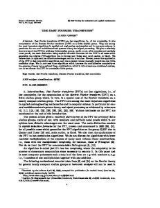
(b) Fig. 1.
50
100
150
200
250
(c)
Example inner loop of the algorithm
A recent breakthrough research from MIT [2] presented an improved algorithm and reduced the time complexity of sFFT √ to O(logn nklogn) which is asymptotically faster than its prior studies. Therefore more applications with “denser” signal spectrum could also achieve performance speedups from the sFFT algorithm. There exists few sFFT implementations [7], [18], [20]. However, they are either a sequential prototype implementation only or an implementation that is barely optimized. To our best of knowledge, we are the first effort of a parallel sFFT algorithm on GPUs and we achieve the best performance so far. III. S ERIAL S PARSE FFT In this section, we present a simplified description of sFFT that is discussed more from a numerical algorithm point of view in [3]. We believe that this will help the reader to understand the complexities in the algorithm from a parallel programming point of view. The functionality of sFFT is hashing the Fourier coefficients into a small number of buckets. Since the signal is sparse in the frequency domain, each bucket is likely to have only one large coefficient, which can then be located (to find its position) and estimated (to find its value). For the algorithm to be sublinear, the binning of Fourier coefficient has to be done in sublinear time. This is achieved by using Gaussian and Dolph-Chebyshev filters, which are concentrated both in time and frequency domain. The algorithm achieves a runtime √ of O(logn nklogn), which is faster than FFT for k up to O(n/logn). We breakdown the sFFT into the following steps: A. Major steps in sFFT Notations For an input signal x ∈ Cn with size n, its Fourier spectrum is denoted by x ˆ. The signal sparsity k, is defined as number of non-zero Fourier coefficients in x ˆ. G ˆ denotes its spectrum in is the flat window function, while G frequency domain. Step 1: Random Spectra Permutation The sFFT bins large Fourier coefficients into a small number of buckets by convolving the permuted input signal with a well-designed filter. To guarantee that each bucket receives only one large Fourier coefficient, which can then be accurately located (to find its position) and estimated (to find its value), the algorithm
permutes the input signal so that the adjacent Fourier coefficients in frequency domain are well separated. In addition, the distance between the original location and permuted location should be large enough so that adjacent coefficients are not be binned into the same bucket. Definition 1. Define the spectra permutation Pσ,τ such that, given an n-dimensional input signal x, an random integer σ that is invertible mod n, and an offset integer τ ∈ [n], \ (Pσ,τ x)i = xσi+τ . Then (P ˆi ω −τ i . σ,τ x)σi = x According to the definition 1, permuted signal in time domain with a shifting factor of τ will lead to phase changes in the frequency domain. This helps in separating the spectra and bin coefficients to the correect buckets. Step 2: Flat Window Function For the sFFT algorithm to be sublinear, only portions of the input signal can perform the FFT operation. Merely sampling partial points of the input signal, however, is impossible because it leads to spectral leakage, i.e., the discontinuities introduced by splicing the signal will appear as sharp components spread out in the frequency domain. To minimize the effects of spectral leakage, sFFT employs a flat window function working as a filter to bin non-zero Fourier coefficients into a small number of p B buckets, where B = O( nk/logn). Specifically, sFFT uses Gaussian and Dolpstartsh-Chebyshev filter, G, because its frequency response is nearly flat inside the pass region and has an exponential tail outside it. So it is unlikely that adjacent Fourier coefficients binned into a particular bucket “leaks” to other. Step 3: Subsampled FFT After the permutation and filtering steps, the permuted signal gets binned into a a smaller number of buckets. Then the reduce-sized FFT is performed. Since we permute the spectra and separate large coefficients, there is a high probability that only one large coefficient potentially exists in each bucket. Next step would be locate and determine its magnitude. Step 4: Cutoff After step 3, each bucket contains at most one potential large coefficient. In the k − sparse signal spectra, the number of buckets, B k, since background noises add to the the signal spectra. We further reduce the amount of computation needed by selecting only the top k coefficients of maximum magnitude. We recover the locations
(b) Run Time vs Sparsity (n=227)
(a) Run Time vs Signal Size (k=1000)
1.6 Elapsed time (sec)
1.4
8
Perm+Filter FFT+Cutoff Location Estimation
7 6 Elapsed time (sec)
1.8
1.2 1 0.8 0.6 0.4
Perm+Filter FFT+Cutoff Location Estimation
5 4 3 2
0.2
1
0 18
19
20
21
22
23
24
25
26
27
Fig. 2.
0 2000 3000 4000 5000 6000 7000 8000 9000 10000 Number of Non-zero Frequencies (k)
Input signal size (2n)
Profiling results for main steps of sparse FFT
and magnitudes only for those top coefficients selected. Step 5: Reverse Hash Function for Location Recovery After removing non-significant coefficients in step 4, the binned coefficients have to be reconstructed, by finding its location in the transformed domain and estimating its magnitude. Since steps 1-4 define a hash function that maps each of the coefficients into one of the B buckets. This function has to be reversed by removing the phase change due to the permutation. Steps 1-5 will run for a number of L = O(logn) location loops with different permutation parameters σ and τ , and return the L sets of locations of candidate coefficients I1 , · · · , IL . For each output of the location inner loop Ii , count the number si of occurrences of each found coefficient i, that is si = |{r|i ∈ Ir }|, and only keep the coefficients which occurred in at least twice in the location loops. I 0 = {i ∈ I1 ∪ · · · ∪ IL |si > L/2}. Step 6: Magnitude Reconstruction In this step, take the r from location loops, essets of locations I 0 and frequencies xc I0 timate each frequency coefficient x bi as x bi = median{xri |r ∈ {1, · · · , L}}. The median is taken in real and imaginary components separately. IV. GPU S PARSE FFT In this section, we present a parallel algorithm for computing the sparse FFT on GPUs. First we profile the sequential sFFT code and plot the time distribution for the major steps in sFFT. Then we discuss the challenges in identifying the suitable parallelization strategies for porting the sFFT onto GPUs. Finally, we introduce how we address the challenges and port each step of sFFT onto GPUs. The optimizations are discussed in Section V. A. Profiling Results Profiling the sequential sFFT shows time distribution for each of the steps when the signal size n increases and sparsity factor k is fixed and vice versa. Figure 2(a) shows the execution time of sFFT with increase in n from 218 (0.26 million points) to 227 (0.13 billion points) with fixed k = 1000. We
see that the permutation+filter (steps 1&2, i.e. permutation + flat window function) increase dramatically when n increases representing the most time consuming steps. Note that the time take by estimation loops (step 6) decreases with an increase in the signal size n, which is counter-intuitive. This is because the size of the estimation loop is determined by the relative signal sparsity. When we fix the signal sparsity k and increase the signal size n, the relative sparsity actually decreases instead. Figure 2(b) shows the time distribution of sFFT when the signal sparsity k increases with fixed signal size n. It is expected to see that the perm+filter and estimation steps gradually dominate the execution time. In this work, although we focus on optimizing primarily the most time consuming steps, we still port the entire algorithm to GPU to avoid the overhead due to bulk volume of PCIe data transfers between CPU and GPU. B. GPU Challenges To achieve maximal performance on the GPU platform, in many cases it requires a deeper understanding of the memory hierarchy and the execution model of the hardware. For instance, it is very important to follow the right memory access pattern to the global memory failing which performance can be affected. To achieve good performance, all threads of a warp should read/write global memory in a coalesced way, i.e., the k-th thread accesses the k-th word in a cache line. Non-coalesced memory access (meaning that it strides across memory lines in the global memory) could lead to more memory transactions than necessary. Because a global memory transaction incurs hundreds of cycles of latency, non-coalesced memory access could significantly degrade the effective throughput of GPUs. An additional challenge is to find an effective way to partition the workload evenly among the hundreds or even thousands of CUDA cores. Parallelism if too fine-grained can result in insufficient balance of work per thread, on the other hand, if a thread has too much workload, this may over-pressure the registers per core and incur more register spilling behaviors. It is very difficult to design an effective sFFT algorithm
that can achieve a high level of parallelism at the same time maximize utilization on the GPU. Parallelizing the algorithm is even more challenging due to loop-carried dependences in the most time consuming kernel. The algorithm being heavily memory-bound leads to relatively small amount of work load per thread, this is yet another performance hinderer. In this paper, we discuss potential solutions to these major challenges. C. GPU Spare FFT Step 1-2: Random Spectrum Permutation and Filtering The sFFT starts with convolving the permuted input signal with a well-designed filter and binning them into a small number of buckets. Algorithm 1 shows the code snippet of the inner loop in the sequential implementation. Noted that the iterations in the loop is filter_size rather than signal size n because the tails of the filter is almost zero, so it is not needed to convolve the signal points to a zero-sized filter. Among the several challenges to parallelize the algorithm for Algorithm 1 Pseudo code for serial permutation and filtering 1: Input: signal[n], f ilter[f ilter size] 2: Output: buckets[B] 3: procedure P ERM F ILTER(signal, f ilter, buckets, B, n,
f ilter size) 4: Initialize: index ← init val 5: while gcd(a, n) 6= 1 do . a,n are co-prime 6: a ← random() mod n 7: end while 8: ai ← mod inverse(a) . ai is modular inverse of a 9: for i ← 1, B do 10: buckets[i] ← 0 . initialize buckets 11: end for 12: . Main body of spectrum permutation and filtering 13: for i ← 1, f ilter size do 14: buckets[i mod B] + = signal[index] × f ilter[i] 15: index ← (index + ai) mod n 16: end for 17: end procedure
GPUs, the first challenge is a loop-carried dependence while updating the variable index that prevents the loop from being parallelized. The index determines and stores the stride distance while permuting the input signal that depends on its previous value. The second challenge is “hash collision” occurring due to multiple permuted signals binned into the same bucket. We use an index mapping algorithm to address the loop-carried dependence issue. Specifically, an observation from Figure 1 is that the values of the index among iterations follow the pattern such that: init_val, (ai + init_val) % n, (2 * ai + init_val) % n for loop iteration i = 0, 1, 2. Therefore, the idea of the index mapping is to directly map the value of index to the loop iterator i without relying on its prior value, as is shown in Figure 3. As a result, the complexity of obtaining the value of index[i] only relies on the loop iterator i and can be therefore parallelized. Regarding the hash collision issue, consider for instance, in Algorithm 1 for loop iterations i = 0, B, 2B, ...,
int index = init_val; for(int i=0; i < filter_size; i++) { ... // Original index calculation index = (index + ai) % n; // After index mapping index = (i * ai + init_val) % n; ... }
Fig. 3.
Index mapping in signal permutation and filter
signal on these points will be binned into the same bucket, leading to the hash collision. Parallelizing this step is a challenge since on GPUs, thousands of threads may update the same bucket simultaneously. Collisions among the threads will serialize the thread execution, seriously impeding the performance. In order to avoid collisions, the conventional way to compute histogram on GPUs is to let each thread keep its own private copy of sub-histogram, local reduction is collision free. In the final stage, combine all sub-histograms into a single histogram using atomic operations. This approach, however, has two drawbacks. First of all, the per-thread approach requires replication of size of B × N bins, where B is number of bins and N is the number of threads. For GPUs with thousands of threads, it is quite obvious that this approach can be extremely expensive in terms of memory space. Furthermore, to minimize the data access latency, most of the implementations [21], [22] utilize on-chip GPU shared memory to store the private sub-histograms. Unfortunately, the size of the shared memory is limited to 48KB even if the state-of-the-art Nvidia Tesla K20x GPUs is considered. This significantly limits the number of bins to 256 or even smaller for a conventional histogram computation [21]. This is a major p limitation for sFFT that has number of buckets, B = nk/logn. For instance, for a signal size of n = 218 and k = 1000, B could be as large as 3,816; B can get larger for even larger input signal size. As a result, for the elements with complex double data types in the buckets, the maximum number of sub-histograms for the size of 48 KB shared memory is 48 ∗ (1024 byte/16 byte)/3816 = 0.8,(16 bytes is the size of an element in the array, which is complex double type) implying that the shared memory could not even hold a single sub-histogram. Some of the histogram computation approaches in [21], [22] use per-warp or per-block replication instead of the per-thread approach, i.e, privatize the subhistograms per each warp or per thread block. Since a warp usually consists of 32 threads and a thread block size could reach to as large as 512 for mainstream GPUs, this approach could significantly relieve shared memory pressure. However, the main drawback of this approach is that it still needs atomic operations to update the sub-histograms within a warp or thread block. The usage of atomic operations can be a major bottleneck to good performance. Another observation with respect to histogram computation is accessing the input data array is predictable, but accessing
Algorithm 2 Pseudo code for GPU permutation and filtering 1: Input: signal[n], f ilter[f ilter size], buckets[B], ai 2: Output: buckets[B] 3: procedure PERM F ILTER(signal, f ilter, buckets,
B, n, f ilter size, ai) 4: rounds ← f ilter size/B 5: for all tid ← 1, B in parallel do 6: Initialize myBucket ← 0 7: for j ← 1, rounds do 8: of f ← idx + B × j 9: index ← of f × ai mod n 10: myBucket+ = signal[index] × f ilter[of f ] 11: end for 12: buckets[tid] ← myBucket 13: end for 14: end procedure
the bucket array is data-dependent (random). The issue with sFFT however, is just the opposite: accessing the input signal is random while accessing the buckets is predictable, as shown in Algorithm 1. Specifically, the number of rounds to access the buckets, filter_size, can be divided into filter_size/B rounds. The filter_size is divisible by B, since both of them are powers of 2. As a result, there is no collision within a round, i.e., intra-round, and collision occurs only across rounds, i.e., inter-round. For instance, updating the buckets when i equals to [0,B] is collision-free and collision only occurs when i = 0, B, 2B, etc.. Based on this observation, we propose a loop partition approach. The basic idea is to partition the original loop iteration into two nested loops, where the outer loop is collision-free and suitable to be mapped to each CUDA thread and the inner loop is processed by one thread. Algorithm 2 shows the pseudo code with loop partition employed for perm+filter step. The outer loop, which has the size of the buckets, is parallelizable and mapped to each CUDA thread, each thread executes the reduction operation for one bucket, independently. Compared to the conventionally GPU histogram reduction approaches, the loop partition approach has mainly three advantages: (a) Bucket replication is not required. Each CUDA thread is responsible for one bucket. (b) Does not require the subhistograms to merge to a single histogram, as a result we avoid using atomic operations (c) Strikes a balance between fine and coarse grained parallelism, since the size of inner loop is very small, each thread does a small amount of work. Step 3: B-dimensional cuFFT After binning the spectra into smaller number of B buckets, a B-dimensional FFT is performed. In our GPU algorithm, we simply employ the cuFFT [5] to perform this function. Furthermore, since this step will be repeated for the number of outer_loops times, of each calculates the same dimension of cuFFT, we use the batched mode of cuFFT and compute cuFFT only once. By sharing the twiddle factors, the batched cuFFT combines the number of outer_loops transforms into one function call, which is much faster than repeatedly calling the cuFFT function. Step 4: Cutoff After we apply the B-dimensional cuFFT,
there are buckets containing potentially large Fourier coefficients in frequency domain. Since the spectra is sparse in frequency, very few of them are potentially large. The objective of the cutoff function is to select the top k largest number of coefficients in the magnitude and store their locations. In the baseline implementation, we apply the sort&select method, as is shown in Algorithm 3. Specifically, we first sort the B buckets in a decreasing order and store the locations of values of the top k largest elements. Here we use the sorting algorithm to perform the cutoff function for several reasons. First of all, sorting is a key building block of many algorithms. It has received a large amount of attention in both sequential and parallel implementations [23]–[25]. For GPU algorithms, the studies in [26]–[28] suggest increase in performance using the right sorting algorithms. In this paper, we use Nvidia’s Thrust library [29] to implement the sort&select algorithm. Thrust is a CUDA-based library performing GPU-accelerated sort, scan, transform, and reduction operations. Using Thrust has several benefits: Thrust is Nvidia’s official library integrated with state-of-the-art CUDA API. As a result, our implementation depending on the Thrust could achieve better robustness, performance and maintains, compared to relying on any other external third party libraries. Nevertheless, sorting is sub-optimal especially for k n. We discuss an alternate technique, in the next section, to fulfill the cutoff function. Algorithm 3 Pseudo code for sort & select 1: Input: buckets[B], k 2: Output: buckets[k], J[k] 3: 4: 5: 6: 7: 8: 9:
. Location and value of the top-k largest elements procedure SORT S ELECT(buckets, J, B, k) for all tid ← 1, B in parallel do J[tid] = tid . Store the index end for ReverseSortByV alue(buckets[B], J[B]) Select(buckets[k], J[k]) end procedure
Step 5: Reverse Hash Functions for Location Recovery The steps from 1-4 define a hash function that maps each coefficient into one of the buckets. The “real” locations of large coefficients need to be reversed by eliminating the phase changes caused by spectrum permutation and filtering. Algorithm 4 shows the pseudo code for the location recovery on GPUs. We launch a number of k threads and each thread independently computes the reverse hash function to recover the location of the potential large coefficients. As described in Section III, steps 1-5 repeats a number of location loops times, so for each inner loop (determining the location), we increment the occurrences(score) of the location recovered. Once the score of the frequency equals to the threshold, we consider this location of coefficient to be large and add it to hits. Magnitude Reconstruction The purpose of this step is that given the locations of large coefficients we need to reconstruct the magnitudes. Since the inner loops are repeated for a number of L loops, given a specific location r ∈ I 0 , we can
Algorithm 4 Pseudo code for GPU location recovery
A. Asynchronous Data Layout Transformation
1: Input: J[k], score[n], a, B 2: Output: hits[num hits] 3: procedure LOC R ECOVERY(J, hits, score, k,
Note that in the first two steps of the sFFT (perm+filter), the algorithm permutes the input signals and bins them into a smaller number of buckets. As shown in Algorithm 2 num hits, a, n, B) 4: for all tid ← 1, k in parallel do (line 10), since the index is calculated as index = (i 5: my J ← J[tid] * ai ) % n, the data reference pattern to the input signal 6: low ← (ceil((my J − 0.5) × n/B) + n) mod n (signal[index]) is largely strided. Such irregular memory 7: high ← (ceil((my J + 0.5) × n/B) + n) mod n reference access pattern leads to non-coalesced global memory 8: loc ← (low × a) mod n accesses on GPUs, which creates memory traffic and is a 9: for j ← low, high do 10: atomicAdd(score[loc], 1) significant bottleneck for achieving good performance. 11: if score[loc] == threshold then Prior work [30], [31] relies on static compiler-based tech12: atomicAdd(num hits, 1) niques that detects the irregularities and reorders the compu13: hits[num hits] ← loc tations at compile time. In sFFT, since the ai is randomly 14: end if generated, the irregular access pattern is dynamic, i.e. it 15: loc ← (loc + a) mod n will remain unknown until run time and even change during 16: end for 17: end for computation. Such dynamic nature severely limits the compiler 18: end procedure techniques to be effectively adopted for the sFFT problem. To coalesce the memory access, we propose an asynchronous data layout transformation technique that can reorder get a set of magnitudes {ˆ xri |i ∈ L}. So the magnitude xˆr is the data on-the-fly. The original non-coalesced kernel is split computed as the median of the candidate magnitudes for all the into two kernels: one performs the data layout transformation L location loops, i.e., median({ˆ xri |i ∈ L}). To parallelize this while the other one accesses the ordered data. In order to hide step, we launch the number of threads equal to num_hits, the overhead of data layout transformation, we take advantage which is the number of potential large coefficients obtained of CUDA concurrent kernel executions where mutiple kernels from the previous step. Each thread computes the reconstruc- execute concurrently on different CUDA streams. Figure 4 tion of the magnitude for a given location independently. shows an example illustrating the use of asynchronous data layout transformation technique to hide the overhead. The Algorithm 5 Pseudo code for GPU magnitude reconstruction remapping kernel creates a chunk of new array, A0 , containing the coalesced data. The new order is created based 1: Input: 2: Output: on a desirable mapping technique between threads and data 3: procedure M AG R ECON() locations, i.e, for loop iteration i, A0 [i] = A[index], where 4: for all tid ← 1, num hits in parallel do A is the original input signal. The second kernel, execution 5: my hits ← hits[tid] kernel, computes the original program but directly accesses 6: n div B ← n/B the reordered data A0 . The chunk size is empirically chosen 7: for j ← 1, outer loops do 8: permuted loc ← ai[j] × myh its mod n to be the bucket size B. So after reordering a chunk of B9: hashed to ← permuted loc/n div B size data, the second kernel launches a number of B threads 10: dist ← permuted loc mod n div B that computes the B elements in a batch. Note that there is 11: if dist > n div B/2 then no data dependence between two remapping kernels (so does 12: hashed to ← (hashed to + 1) mod B execution kernel), so remapping the data chunk δ and δ +i can 13: dist ← dist − n div B 14: end if happen concurrently. The maximum depth of the concurrency 15: dist ← (n − dist) mod n depends on the CUDA compute capability that is different for 16: mag[j] ← buckets[j][hashed to]/f ilter f req[dist] different GPU architecture. For GK110 used in this paper, the 17: end for maximum number of concurrent executed kernels is 32. 18: sort(mag, outer loops) 19: median ← (outer loops − 1)/2 20: loc[tid] ← my hits 21: val[tid] ← mag[median] 22: end for 23: end procedure
V. O PTIMIZATIONS In Section IV, we had presented some baseline optimizations to parallelize sFFT for GPUs. We also discussed some architectural challenges that the GPUs pose. In this section, we present some improved optimization techniques for the most time consumed portions of the algorithm.
B. Fast K-selection Algorithm In step 4 of the algorithm, we applied a cutoff function to select the k largest elements from a set of B buckets. As described in Section IV, we basically sort the entire list and select the k largest elements from the sorted list. However, when the amount of data grows sorting the entire list becomes more and more expensive: BlogB operations with a typical sorting algorithms only leads to top k useful information, where k B. Therefore, one could expect to accomplish this task in a time proportional to the data size, i.e., at linear time. Beyond sFFT, there also exists numerous applications requiring this possibility where only the k largest values in a
Remapping Kernel reorder chunk reorder chunk
VI. E VALUATION +1
reorder chunk
+2
reorder chunk
Streams
...
+3
...
Execution Kernel
...
Fig. 4.
...
Time
Asynchrnous data layout transformation
We evaluate the performance of sparse FFT on GPUs in this section. We compare the performance with cuFFT, which is the fastest implementation for computing the dense FFT with the runtime of O(nlog(n)) on NVIDIA GPUs. We also evaluate on both of our implementations: the baseline implementation described in Section IV and the effects of optimizations discussed in Section V. For completeness, we also compare with OpenMP version of sFFT (PsFFT) on multicore CPUs from our prior work [6] and the parallel FFTW, one of the most widely used dense FFT library for multicore CPUs. A. Experimental Setup
Input: buckets[B], k Output: J[k] procedure FAST S ELECT(buckets, J, B, k) Initialize: count ← 0 for all tid ← 1, B in parallel do key ← tid value ← buckets[tid] if value ≥ thresh then myCount ← atomicAdd(count, 1) J[myCount − 1] ← key end if end for end procedure
list are retained while the remaining entries are ignored or set to zero [32], [33]. Linear-time fast selection algorithms have received a large amount of attention in sequential and parallel implementations [23], [34]. For GPU algorithms, Alabi et. al [35] proposed a BucketSelect algorithm. Similar to bucket sorting, the proposed algorithm works well only when the data is uniformly distributed, i.e., the number of elements assigned to each bucket is roughly equal. For the sFFT algorithm, however, only very few of the buckets are large while the rest of them are almost empty. In this paper, we propose a fast selection algorithm which is simple but effective in sFFT. As shown in Algorithm 6, we assign a number of B threads and each thread processes one element in the buckets. If the value in the buckets is greater than the threshold, the element is chosen and index is stored. It is noted that the choice of the threshold is important for the algorithm. If it is too small, many small coefficients will be picked up and falsely treated as “large”. On the other hand, if the threshold is too large, some useful large coefficients will be lost. In this paper, we choose the threshold based on a key observation: only the k out of B buckets are large while rest of them are very small with similar order to amplitude. Consequently, the value of the threshold is chosen to be in the same order of the “small” noise coefficients, of which the value could be empirically obtained from past experience. Most of the time, this approach will yield slightly more than the number of k elements, but this is ignored in the step 4 of the sFFT.
Table I and Table II show the experimental configurations for this evaluation. We evaluated the cusFFT on NVIDIA Kepler K20x GPU and Intel Sandy Bridge E5-2640 processor. The CUDA compiler is NVIDIA’s nvcc compiler with version 5.5. The CPU compiler we chose is Intel compiler 13.1 which delivers the best performance on Intel Sandy Bridge architecture. We have also used -O3 optimization flag for both CPU and GPU compilers. The FFTW library used is the latest 3.3 version with multi-threading configured. B. Experimental Results In Figure 5(a), we have fixed the sparsity parameter k = 1000. We report the runtime of the algorithms compared for different signal sizes n ranging from 218 to 227 . We plot the average execution time for cusFFT baseline version, optimized version, cuFFT, as well as OpenMP sFFT(PsFFT) and FFTW on CPUs. As expected, Figure 5(a) shows that the runtimes of cusFFT and cuFFT are approximately linear in the log scale. However, the slope of the line for cusFFT is less than the slope for cuFFT, which is a result of cusFFTs sub-linear runtime. The figure also shows that for signal sizes n > 222 both baseline and optimized versions of cusFFT are faster than the cuFFT in recovering the exact 1000 non-zero coefficients. The gap becomes bigger when the data size grows, meaning that speedup of cusFFT will be more than than cuFFT. Figure 5(b) shows that we fix the signal size to n = 227 and evaluate the average execution time of cusFFT while the number of non-zero frequencies k ranges from 100 to 1000. Since both cuFFT and FFTW have a runtime of O(nlogn), they are independent of the number of non-zero frequencies k, as can be seen in Figure 5(b). Nevertheless, as and when the sparsity k increases, the execution time of sFFT increases very slowly. In Figure 5(c), we plot the speedup of cusFFT over cuFFT. From the figure we can see that the speedup grows very fast with the signal size n, which shows that our cusFFT algorithm benefits a lot on large signal size. For the signal size n = 227 , the cusFFT is 15x and over 9x faster than the cuFFT for the optimized and baseline version, respectively. We also compare cusFFT with the parallel FFTW and the OpenMP version of sFFT (PsFFT) we developed before on multicore CPUs. Figure 5(d) shows the speedup of the cusFFT over the parallel FFTW on CPUs. From the figure
TABLE I GPU TEST- BENCH GPU Type Tesla K20x
CUDA Capability 3.5
CUDA Cores 2688 cores / 14 SMs
Processor Clock 732 MHz
Shared Memory 64 KB
Global Memory 6 GB
Memory Bandwidth 250 GB/s
TABLE II CPU TEST- BENCH Processor Intel(R) Xeon(R) CPU E5-2640
Architecture Sandy Bridge
Cores 6
Processor Clock 2.50 GHz
we could see that the optimized cusFFT is 0.5x to 29x faster to parallel FFTW for the signal size ranges from 218 to 227 . In Figure 5(e), we compare the speedup of cusFFT over the PsFFT. It can be seen from the figure that the speedup grows with the signal size, to the peak speedup 6.6x for n = 224 , and then slightly goes down when the signal size becomes larger. That is mainly due to the data transfer time between the host and device offsets the performance gains on the GPU computation. But the average speedup of the cusFFT on GPUs is over 4x faster than PsFFT on CPUs. Figure 5(a) to Figure 5(e) also show that the optimized cusFFT is on average 2x faster to the baseline version, which proofs the effects of optimization strategies discussed in Section V. Last, we also check that cusFFT’s good performance is not at the expense of reduced accuracy. Essentially, our cusFFT ensures the same numerical accuracy to the original sequential algorithm. In addition, we compare the output of cusFFT, x ˆ, with the FFTW, yˆ, and compute the L1 error, whichPis the accumulated error per large coefficient defined as k1 0