providing a trustworthy platform for microkernel programmersâcan be proven cor ..... memory regions happens only within the dedicated primitives of the kernel.
Electronic Notes in Theoretical Computer Science 217 (2008) 151–168 www.elsevier.com/locate/entcs
CVM - A Verified Framework for Microkernel Programmers Tom In der Rieden1 Deutsches Forschungszentrum f¨ ur K¨ unstliche Intelligenz (DFKI) Saarbr¨ ucken, Germany
Alexandra Tsyban1 Computer Science Dept. Universit¨ at des Saarlandes Saarbr¨ ucken, Germany
Abstract CVM (communicating virtual machines) is a computational model for concurrent user processes interacting with a generic microkernel—supporting virtual memory—and devices. In this paper, we introduce the computational models needed to define CVM. Furthermore, we describe how CVM can be implemented by means of a concrete kernel, thus providing a trustworthy platform for microkernel programmers. Last but not least, we give an overview on the model formalization and implementation correctness proof, which has been conducted in the interactive theorem prover Isabelle for the most part. An endeavor like this is tedious and of a considerable complexity. Thus, we do not try to present all details, but provide references to publications covering specific aspects. Keywords: Operating Systems, Microkernel, Systems Verification, Isabelle, Theorem Proving
1
Introduction
Operating systems are crucial components in nearly every computer system. They provide plenties of services and functionalities, e.g. managing inter-process communication, device access, and memory management. Obviously, they play a key role in the reliability of such systems and in fact, a considerable share of hacker attacks target operating system vulnerabilities. Thus, proving a computer system to be safe and secure requires to prove its operating system to be safe and secure. 1
This work was partially funded by the German Federal Ministry of Education and Technology (BMBF) in the framework of the Verisoft project under grant 01 IS 07008. The responsibility for this article lies with the authors.
1571-0661/$ – see front matter © 2008 Elsevier B.V. All rights reserved. doi:10.1016/j.entcs.2008.06.047
152
T. In der Rieden, A. Tsyban / Electronic Notes in Theoretical Computer Science 217 (2008) 151–168
At first sight, this appears to be a mission impossible because of the sheer size of operating system implementations. For example, the Linux 2.6.0 kernel released in late 2003 has nearly 6 million lines of code. Yet, the idea of having a small and reliable kernel is not new and has led to the development of so-called 2nd generation microkernels like L4 [16]. Microkernels offer elementary, but sufficient functionality, and can therefore be of relatively small size. For instance by using them as a trusted platform, we can run two operating systems on top of it, one small and reliable for critical applications, and a conventional one for all other tasks [24]. In this paper, we describe how a whole framework, featuring virtual memory support, memory management, system calls, user defined interrupts, etc.—thus providing a trustworthy platform for microkernel programmers—can be proven correct. We introduce a computational model called CVM (communicating virtual machines), that formalizes concurrent user processes interacting with a generic (abstract) microkernel and devices. To establish interaction, the abstract kernel features special functions called CVM primitives, which are invoked by the user processes and alter process or device configurations, e.g. by copying data from one process to another. By linking a CVM implementation to an abstract kernel, we obtain a concrete kernel (‘personality’). For each layer in the computer system—hardware, devices, user processes, and abstract kernel—we define a formal model. Implementation correctness is defined by several simulation relations between these layers. The proofs are conducted in the interactive theorem prover Isabelle/HOL [22] and have already been completed to a large extent. CVM is used in the Verisoft project [29] in two personalities: (i) VAMOS is a microkernel used in an academic stack, where on top of it a simple operating system (SOS) is running, and (ii) OLOS, an OSEKtime-like operating system, is used in a distributed automotive real-time system establishing eCall functionality [13]. The remainder of this paper is structured as follows. In Sect 2 we list some related work. Sect. 3 introduces some notation needed in Sect. 4 to define our models formally. We present a generic framework for devices in Sect. 4.1. In particular, we show how physical machines and external devices can be coupled formally (Sect. 4.2). User processes are modeled by assembler machines running on virtual memory (Sect. 4.3), while computations of the abstract kernel are defined by C0 semantics (Sect. 4.4). In Sect. 5 we sketch the construction of the concrete kernel containing the CVM implementation. The simulation relations that establish CVM implementation correctness are described in Sect. 6. The status quo of the formal verification is presented in detail in Sect. 7. We conclude in Sect. 8.
2
Related Work
First attempts to use theorem provers to specify and even prove correct operating systems were made as early as the seventies in PSOS [20] and UCLA Secure Unix [32]. However a missing—or to a large extend underdeveloped—tool environment made mechanized verification futile. With the CLI stack [4], a new pioneering ap-
T. In der Rieden, A. Tsyban / Electronic Notes in Theoretical Computer Science 217 (2008) 151–168
153
proach for pervasive system verification was undertaken. Most notably, the simple kernel KIT was developed and its machine code implementation was proven to be correct. Compared to modern kernels KIT was very limited, in particular, it lacked interaction with devices. The project L4.verified [9] focuses on the verification of an efficient microkernel, rather than on formal pervasiveness, as no compiler correctness or accurate device interaction is considered. The microkernel is implemented in a larger subset of C, including pointer arithmetic and an explicit low-level memory model [31]. However with inline assembler code we gain an even more expressive semantics as machine registers become visible if necessary. So far, only exemplary portions of kernel code were reported to be verified, the virtual memory subsystem uses no demand paging [30]. For code verification L4.verified relies on the Verisoft’s Hoare environment [26]. In the FLINT project, an assembly code verification framework is developed and code for context switching on a x86 architecture was formally proven [21]. Although a verification logic for assembler code is presented, no integration of results into high-level programming languages is undertaken. The VFiasco project [12] aims at the verification of the microkernel Fiasco implemented in a subset of C++. Code verification is performed in a embedding of C++ in PVS and there is no attempt to map the results down to the machine level.
3
Notation
We use f : A � B to denote a partial mapping f from sets A to B, while g : A → B stands for a total mapping. We denote the concatenation of bit strings a ∈ {0, 1}n and b ∈ {0, 1}n by a ◦ b. For bits x ∈ {0, 1} and positive natural numbers n ∈ N+ , we define inductively x1 = x and xn = xn−1 ◦ x, e.g. 05 = 00000 and 12 = 11. For x ∈ {0, 1}n , x[i], 0 ≤ i < n denotes the bit at position i of the bit string. Ni with i ∈ N+ denotes the natural interval [0, i − 1]. For finite sequences seq : N � T , we use shorthand notation seq = hd; tl where hd denotes the head of the sequence, i.e. the element seq[0], and tl the remaining elements.
4
Computational Models
We have developed a generalized framework to model different devices in a uniform way (Sec. 4.1). Physical machines (Sec. 4.2) are used to specify the underlying microprocessor hardware. User process computations are modeled by assembler semantics (Sec. 4.3), abstract kernel computations by C0 semantics (Sec. 4.4). Finally, we combine the above computational models to specify CVM (Sect. 4.5). 4.1
Devices
We use devices in two ways in CVM. First, the page fault handler described in Sect. 5.3 uses a hard disk as swap device. Second, we offer a range of typical devices accessible by user processes through special kernel calls. Currently, we support models for five different device types: (i) a hard disk, e.g. used as the swap device for memory virtualization [11], (ii) a timer, which can be used for scheduling
154
T. In der Rieden, A. Tsyban / Electronic Notes in Theoretical Computer Science 217 (2008) 151–168 mif i mif o mif i Processor
mif o
eif o1 DEV1 DEV2
eif i1 eif o2 eif i2
Environment
mif i
eif odmax DEVdmax mif o eif idmax Fig. 1. Device Model
user processes, (iii) a network interface, (iv) an UART serial interface, which can be used to set up a terminal [1], and (v) an automotive bus controller, which is used in Verisoft’s Automotive subproject [14,13]. Device communication happens on many different layers throughout our stack. Nevertheless, in order to establish a uniform way of interacting with devices, we have developed a generic device framework featuring standardized transition functions for all layers. For each device type, we define a specific device configuration, e.g. chd for hard disks. The set of all specific device configurations (including a generic error state ⊥) is denoted by Conf sdevs . Furthermore, we define the set of device IDs by DID = N+ dmax+1 , whereas dmax is fixed and determines the maximal number of devices. Formally, the generalized device configuration is defined by the mapping Conf devs : DID → Conf sdevs . Devices are memory-mapped and can communicate in two directions, namely with the processor and with the environment (e.g. with a user or a screen). Thus, we define two transition functions, one for internal and one for external communication. The generalized internal transition function is parameterized over inputs from the processor (Mifi ). One element of the processor input is defined by a tuple mifi = (id, rd, wr, ad, count, data), whereas (i) id ∈ DID denotes the device ID, (ii) rd ∈ {0, 1} denotes the read flag, (iii) wr ∈ {0, 1} denotes the write flag, (iv) ad gives the device port where to read from or where to write to, and (v) data finally specifies the data to be written if wr = 1. Furthermore, internal steps do not only yield a successor device configuration, but also output to the processor (Mifo ⊆ N) and, potentially, to the environment, which is specific for each device type: Eifo = {Eifo hd , Eifo abc , . . .}. Now we can formally define the generalized internal transition function δdint : Conf devs × Mifi → Conf devs × Mifo × Eifo. Input from the environment is also device type specific; We specify the generalized set of environment input by Eifi = {Eifi hd , Eifi abc , . . .}. Again, devices may generate output. The external transition function is given by δdext : Conf devs × DID × Eifi → Conf devs × Eifo. Of course this way of dealing with devices is not the only possible on; modern architectures mostly rely on devices with direct-memory access (DMA). Yet, this makes modeling much more difficult and would require considerable changes on the hardware implementation. First, either the processor would not be the sole bus master any longer, but I/O MMUs would have to guard the bus, or one would have
T. In der Rieden, A. Tsyban / Electronic Notes in Theoretical Computer Science 217 (2008) 151–168
155
to trust devices not to access sensitive data; second, DMA regions would have to be excluded from caching. Since these regions are set up dynamically, this would require hardware support for explicit cache flushing.
4.2
Physical machines and instruction set architecture
The lowest layer in our stack is given by the architecture of the underlying VAMP microprocessor [6]. The VAMP provides a single-level address translation mechanism [8,10] and supports memory-mapped devices [1,11]. In order to realize memory virtualization, the VAMP runs in two modes: user mode and system mode. In user mode, all addresses are virtual and have to be translated first before accessing memory [7]. However, in system mode, we deal with physical addresses that can be used without translation. In our scenario, the microkernel runs in system mode while the user processes run in user mode. The processor and the devices may either progress individually or communicate with each other. Communication is established either by the processor executing a memory operation to a special memory region assigned to devices (see Fig. 3) or by the device causing an external interrupt. Physical machines are the hardware model for a system programmer. Due to space limitations, we will only introduce the relevant parts here. A physical machine configuration cphys comprises the registers, the program counters, and the memory content. The register file is split into two parts: (i) gpr : {0, 1}5 → {0, 1}32 , the general purpose register file, and (ii) spr : {0, 1}5 � {0, 1}32 , the special purpose register file. For shorthand notation, we use symbolic names for special purpose registers, e.g. Edata for spr(00101). In order to implement the delayed branch mechanism as described in [17], we specify a program counter pc ∈ {0, 1}32 and a delayed program counter dpc ∈ {0, 1}32 . Finally, there is a word-addressed physical memory pm : {0, 1}30 � {0, 1}32 . We formally denote a physical machine configuration by the tuple cphys = (gpr, spr, pcp, dpc, pm). An instruction set architecture (ISA) is given by a transition function δphys , that maps a configuration cphys and external event signals eev ∈ {0, 1}dmax to a next configuration c�phys = δphys (cphys , eev). Due to space limitations, we will not give a full formal definition of the ISA transition function, but only an idea of it. The transition function depends on the special purpose register mode, where mode = 0 denotes system mode and mode = 1 denotes user mode. For system mode, the transition function is simply defined by the instruction to which cphys .dpc points (see [5,17]). In user mode, memory accesses are subject to address translation: they either cause a page fault or are redirected to the translated physical address pma(cphys , va) for a given virtual address va. For details on VAMP address translation see [8]. In order to define δphys (cphys , eev) more formally, we need some helper functions: (i) I(cphys ) = cphys .pm(cphys .dpc) denotes the instruction to be executed in configuration cphys , (ii) predicates ?lw(cphys ) and ?sw(cphys ) distinguish I(cphys ) being a ’load word’ or a ’store word’ instruction, (iii) RS1(cphys ), RS2(cphys ),
156
T. In der Rieden, A. Tsyban / Electronic Notes in Theoretical Computer Science 217 (2008) 151–168
and RD(cphys ) are returning the general purpose register operands of I(cphys ), (iv) imm(cphys ) returns the immediate constant of I(cphys ), and (v) ea(cphys ) = cphys .gpr(RS1(cphys )) + imm(cphys ) specifies the effective address of I(cphys ), i.e. its memory operand. Note, that for CVM, only the kernel running in system mode interacts directly with devices, thus address translation does not affect. Devices are memory mapped, i.e. a part of the memory is shared by both the processor and the devices (cf. Fig. 3). We denote the set of addresses in this part of the memory by DIO. Let the predicate ?int(i) denote, if the device with ID i is in an interrupt state. We can now define the external event signals as eev =?int(dmax)◦?int(dmax − 1) ◦ . . . ◦?int(1). Let us introduce an input alphabet I = (DID × Eifi ) ∪ {0} and an output alphabet O = Eifo ∪ {ε}. Formally the combined transition function of physical machines and devices δp&d (cphys , cdevs , in) = (c�phys , c�devs , out) is defined for in ∈ I and out ∈ O as follows. For external device input (in = 0), we execute the external device transition function, thus c�phys = cphys and (c�devs , out) = δdext (cdevs , in). For processor steps (in = 0), we distinguish between steps with device interaction, i.e. ea(cphys ) ∈ DIO, and without device interaction: (i) in the former case, we execute both the processor and the internal device transition function: c�phys = δphys (cphys , eev) and (c�devs , mifo, out) = δdint (cdevs , mifi ). If ?lw(cphys ), we set c�phys .gpr(RD(cphys )) = mifo, otherwise we discard mifo. (ii) In the latter case, we execute the transition function of the processor: c�phys = δphys (cphys , eev) and (c�devs , out) = (cdevs , ε). Here, mifi is obtained by a helper function dec(ea(cphys )) = (i, ad) returning the device id i and port ad for a given effective address, such that mifi = (i, ad, ?lw(cphys ), ?sw(cphys ), cphys .gpr(RD(cphys ))). n The n-step transition function δp&d takes initial configurations cphys and cdevs , and a input sequence ins of length m, with elements mi ∈ I and m ≥ n. While exen cuting single steps, δp&d generates an output sequence outs of length m and elements n 0 (c in O. We define δp&d recursively: (i) δp&d phys , cdevs , ins) = (cphys , cdevs , ε), and i+1 � � i (ii) δp&d (cphys , cdevs , ins) = δp&d (cphys , cdevs , ins(i + 1)) with δp&d (cphys , cdevs , ins) = � � (cphys , cdevs , outs) 4.3
Assembler Semantics
User processes are applications running on top of the microkernel. Given that we also want to consider malevolent (hacker) applications, we restrain from any programming restrictions imposed by C and model all processes as assembler machines. More precisely, since the microkernel is providing memory virtualization and these applications run on a uniform virtual memory, we will use virtual assembler machines. A virtual machine configuration cASM is closely related to the physical machine configuration describing the hardware. It still comprises the register files and the program counters. We consider register numbers as naturals and their contents as integers. Furthermore, only a subset of the special purpose registers available in the real hardware is visible here and the instruction set is limited. We formally define the register files (similar to Sect. 4.2) as (partial) mappings,
T. In der Rieden, A. Tsyban / Electronic Notes in Theoretical Computer Science 217 (2008) 151–168
157
i.e. gpr : N32 → Z and spr : N32 � Z, and the two program counters dpc, pcp ∈ N. The memory is given by mm : N � Z, such that the overall assembler configuration is specified by the tuple cASM = (gpr, spr, pcp, dpc, mm). The transition function, which maps a given assembler configuration cASM either to its successor configuration or to an error state ⊥: δASM : Conf ASM → Conf ASM ∪ {⊥}, is defined over the current instruction to which (dpc.mm(c.dpc)) points. For example, the error state can be reached if the user process tries to access a restricted special purpose register. n Let δASM : Conf ASM → Conf ASM ∪ {⊥} denote the function that applies the 0 (cASM ) = cASM and transition function n ∈ N times. We define inductively (i) δASM i+1 � i � (ii) δASM (cASM ) = δASM (cASM ) if δASM (cASM ) = cASM and c�ASM = ⊥, else ⊥.
4.4
C0 Small Step Semantics
C0 is the C-like imperative programming language developed and widely used in Verisoft. It features sufficient functionality to implement system software and applications, yet having a concise formal semantics which allows for the—more or less—efficient verification of code with several thousands lines, e.g. a non-optimizing compiler and a simple email client [23,3]. A C0 program is identified by its functions—including information about their list of parameters and local variables—, the type name environment and the list of global variables. C0 supports four elementary types (Bool, Integer, U nsigned and Char) and allows for non-elementary, recursive data types: Arr(l, t) denotes the array with l elements of type t and, for types ti and component names ni , Struct([(n0 , t0 ), . . . , (nl , tl−1 )]) denotes a structure type with l components. C0 pointers are denoted by P tr(tn) where tn stands for a type name defined in the type name environment tenv, a mapping tenv : Σ+ � ty mapping type names to types. The procedure table contains the information about all functions of a C0 program. Formally, it is a partial mapping ptable : Σ+ � f desc of function names to their corresponding descriptors, containing information on function body, parameters, local variables and return type. The global variables are defined by a sequence of variable names and their associated types: st : N � Σ+ × ty, called symbol table. We will not discuss in detail C0 statements (Stmt) and expressions (Expr). The definitions of both are straightforward and are presented exhaustively in [15]. A C0 configuration cC0 = (mem, pr) consists of the memory configuration mem—storing information about the (possibly dynamically allocated) program variables and their values—and the program rest pr. Variables are represented in a generalized way as so-called g-vars, defined inductively as: a global variable of name x as gvargm (x), a local variable of name x in the i-th stack frame as gvarlm (i, x), and a nameless heap variable with index i as gvarhm (i). If s is a g-var of structural type, then its component with name cn is also a g-var: gvar(s, cn). Similar, for a g-var a of array type, its i-th element is also a g-var: gvar(a, i). A memory configuration is given by a triple consisting of (i) a global memory frame mem.gm : mframe,
158
T. In der Rieden, A. Tsyban / Electronic Notes in Theoretical Computer Science 217 (2008) 151–168
(ii) a local memory stack mem.lm : N � mframe × gvar 2 , and (iii) a heap memory frame mem.hm : mframe. Each frame contains a symbol table and a content ct : N � mcell , mapping addresses to typed memory cells. Memory cells can store the value of an elementary type variable, whereas pointers are represented by a g-var or the null pointer value Null ; values of aggregate variables are stored in consecutive memory cells. The second component of a C0 configuration is the program rest, a sequence of statements still to be executed: pr = s1 , . . . , sn with si ∈ Stmt. Given a type name environment te and a procedure table pt, the transition function maps the current C0 configuration either to its successor configuration or to an error state ⊥: δC0 : tenv × ptable × Conf C0 → Conf C0 ∪ {⊥}. δC0 is defined inductively over the program rest (see [15] for a detailed definition). n , which executes the transition function n times, by induction on n: We define δC0 i+1 0 (te, pt, c � i (i) δC0 C0 ) = cC0 (ii) δC0 (te, pt, cC0 ) = δC0 (te, pt, cC0 ), if δC0 (te, pt, cC0 ) = � � cC0 and cC0 = ⊥, else ⊥. 4.5
CVM Semantics
Communicating virtual machines (CVM) are a computational model for a fixed number of processes. The processes can interact with each other and with a fixed number of devices, whereas all communication is handled by a generic abstract microkernel offering various specific kernel calls (CVM primitives). So far, there is no support for shared memory, neither between devices and processes nor between processes themselves. We use assembler semantics as introduced in Sect. 4.3 to model user process computations and the C0 semantics from Sect. 4.4 for the computations of the abstract kernel. Device behavior is defined by the semantics described in Sect. 4.1. A CVM configuration cCVM = (kernel, proc, devs, sr, cup) comprises the following five components: (i) Let PID = N+ pmax+1 denote the set of user process IDs with a fixed pmax. Then, a user processes configuration procs is formally a mapping of process IDs to assembler configurations: procs : PID → Conf ASM . (ii) The kernel part is specified by a type name environment, a procedure table, and a C0 configuration: kernel = (tenv, pt, conf ). (iii) The device configuration is given by a generalized device configuration devs. (iv) cup ∈ PID ∪ {0} specifies the current process ID or, in case of cup = 0, the kernel. (v) sr ∈ {0, 1}dmax−1 , the interrupt mask for the devices. If sr[i] = 0, then interrupts of the device with ID did = i + 2 are masked 3 . In each CVM step, either the kernel, or one user process, or one device progresses. One step in a CVM computation is defined by the transition function δCVM : Conf CVM × I → (Conf CVM ∪ {⊥}) × O, where ⊥ denotes the error state. In the following definitions, we only mention components that are changing in one step of the computation. 2
local memory frames have an additional g-var defining the memory location where the function return value is to be stored 3 Note, that the hard disk used for swapping (device ID did shd = 1) is not visible in the CVM specification.
T. In der Rieden, A. Tsyban / Electronic Notes in Theoretical Computer Science 217 (2008) 151–168
159
reset ?P rim primitive
init
kernel ¬?P rim ∧ ¬?Return
JISR
?Return∧ cup �= 0
¬JISR user step
Fig. 2. CVM Control Flow
Given a CVM configuration cCVM and a parameter in: if in = 0, we execute the external transition function of the device part of the CVM configuration cCVM .devs as described in Sect. 4.1: δdext (cCVM .devs, in) = (c�CVM .devs, out). For in = 0, execution depends on the value of cCVM .cup: if cCVM .cup = i > 0, the user process cCVM .procs(i) makes a step, otherwise the kernel progresses. Let the predicate JISR(cASM , cdevs ) ∈ {0, 1} denote, that an interrupt occurred in the current user process configuration cASM and device configuration cdevs w.r.t. the interrupt mask cCVM .sr. Then we compute the (masked) exception cause mca(cASM ) ∈ N and a potential parameter edata(cASM ) ∈ N (e.g. in case of a trap exception). Details on JISR, mca, and edata can be found in [8,17]. For ¬JISR(cCVM .procs(cCVM .cup), cCVM .devs), we execute the transition function δASM as described in Sect. 4.3: c�CVM .procs(cCVM .cup) = δASM (cCVM .procs(cCVM .cup)). Otherwise, a visible interrupt has occurred and kernel execution starts at the entry point given by the C0 function kdispatch with parameters mca and edata. We set cCVM .cup = 0 and the kernel’s program rest to the function call c�CVM .kernel .conf .pr = SCall (kret, kdispatch, mca(cASM ), edata(cASM )) where kret denotes the return variable and SCall is the C0 function call statement. After booting and after an interrupt, kernel execution starts by calling the function kdispatch. Note, that while the kernel runs, interrupts are disabled, i.e. our kernel is non-interruptible (’non-preemptive’). If cCVM .cup = 0 and the kernel program rest does not start with a function call to a CVM primitive , we simply execute the C0 transition function as described in Sect. 4.4: c�CVM .kernel = δC0 (cCVM .kernel). Otherwise, we have cCVM .kernel .conf .pr = ESCall (v , prim, expr1 , . . . , exprn ); r for a CVM primitive prim, an integer return variable v and unsigned expressions expr1 , . . . , exprn ∈ Expr . Here, ESCall is the C0 statement for external function calls, i.e. functions with declarations but without a body (Sect. 5 explains how to get a fully implemented kernel). Each primitive prim is specified by a function primS , which takes n natural arguments and a CVM configuration cCVM , returning an updated CVM configuration c�CVM or the error state ⊥. Let evalr be the evaluation function for righthand side C0 expressions as defined in [15]. Then, we compute for 1 ≤ i ≤ n: vali = evalr (cCVM .kernel, ei ) and set (c�CVM ) = primS (cCVM , val1 , . . . , valn ). For example, CVM provides primitives (i) Reset and Clone for process initialization, (ii) Alloc and Free for increasing and decreasing memory of an user process, (iii) Copy to copy data from one process to another, (iv) GetGPR and SetGPR to
160
T. In der Rieden, A. Tsyban / Electronic Notes in Theoretical Computer Science 217 (2008) 151–168 Device IO
System Memory
User Processes
User Memory
Zero Fill Page Kernel Heap Kernel Stack Kernel Data Kernel Code Zero Page
System Memory
Fig. 3. CVM Memory Map
read and write registers of user processes, (v) GetWord and SetWord to read from and write to a user process memory address, (vi) InWord and OutWord for device communication, and (vii) SetMask for setting the CVM interrupt mask. For a full list of primitives see [27]. Due to lack of space, we exemplify by the specification of SetGPR: Given a configuration with kernel program rest ESCall (v, SetGPR, expr1 , expr2 , . . . , expr5 ); r. We set SetGPR S (cCVM , pid, i, y) = c�CVM with (i) c�CVM .proc(pid ).gpr (i ) = y, (ii) c�CVM .kernel .conf .pr = r, and (iii) c�CVM .kernel .conf .mem = mem update(cCVM .kernel .conf .mem, v , 0 ) with the C0 memory update function as defined in [15]. Note, that since the whole stack runs on one single processor, it is legal to assume that either the kernel or an user process perform a step. This is not that obvious for the devices. Remember that devices are memory-mapped and access to these memory regions happens only within the dedicated primitives of the kernel. These primitives are written in assembler, hence steps in the kernel and on the physical machine have the same granularity: one instruction. Additionally, the actual synchronization with the device can be mapped down to one single instruction, namely a load word or store word instruction. All other steps during kernel execution are independent from the device computation. This means, all interleavings possible between physical machine steps and devices—as seen in Sect. 4.2—are also possible on between the kernel and the devices.
5
CVM Implementation
In this section, we will give an overview on the CVM implementation details and how to merge such an implementation with the abstract kernel in order to obtain a compilable and thus executable kernel. 5.1
Data Structures
To simulate virtual machines and multi-processing, the CVM implementation has to maintain certain data structures: (i) in the kernel global memory (kernel data), we store an array of process control blocks pcb[i], i ∈ PID for all user processes. One process control block has components pcb[i].r for each register and the program counters of cphys , (ii) the global memory variable cup keeps track of the current user
T. In der Rieden, A. Tsyban / Electronic Notes in Theoretical Computer Science 217 (2008) 151–168
161
process as specified in cCVM .cup and similarly, sr for cCVM .sr, (iii) in the global memory variable kheap, we store the end address of the kernel heap, (iv) the array ptspace on the kernel heap holds the page tables of all user processes, and (v) data structures of the page-fault handler (see Sect.5.3) necessary for the management of physical and swap memory. 5.2
Entering and Leaving System Mode
Whenever we enter system mode, i.e. the kernel starts to execute, we initialize its program rest with cCVM .kernel .conf .prog = init. In all cases but reset, init will take the current process and store its registers into the corresponding control block pcb[cup]. Then, the kernel is initialized and the CVM dispatcher cvmdispatch is called with parameters pcb[cup].eca, pcb[cup].edata, and pcb[cup].edpc. As mentioned in Sect.4.5, interrupts are to be invisible in system mode. We achieve this by zeroing the status register cphys .SR. In case of a page fault, the page fault handler is invoked by cvmdispatch. Otherwise we continue with a call to the abstract kernel dispatcher kdispatch with parameters pcb[cup].eca and pcb[cup].edata. To leave system mode and with i ∈ PID being the user process to be started, we set cup = i and restore the process from its control block pcb[i]. Finally, we leave kernel execution with a return from exception instruction (rfe). Note, that a scheduler is not part of the concrete kernel, i.e. the abstract kernel has to take care of handling timer interrupts. Thus, we are not giving any guarantees 5.3
Page Fault Handler
For pcb[cup].eca = 8, the user process with ID cup has caused a page fault on fetch interrupt (pff ), i.e. the process’ delayed pc points to an address not present in physical memory. Thus, the page fault handler is called with parameters cup and pcb[cup].edpc. For pcb[cup].eca = 16, we are dealing with a page fault on load/store (pfls), i.e. a memory operation was accessing an address not present in physical memory. In this case, cvmdispatch invokes the page fault handler with parameters cup and pcb[cup].edata. For details on the paging algorithm used in Verisoft see [2]. 5.4
CVM Primitives
The implementation of the various primitives is straightforward. Some of them are only updating the process control blocks of tasks and are therefore implemented in pure C0 . Other primitives—e.g. those copying memory from one process to another—are manipulating data structures not visible in C0 . In these cases, hardware-specific assembler code portions are inevitable. We inline them directly into the C0 code with a special ASM statement. 5.5
Abstract Linker and Concrete Kernel
As we have seen in the sections before, it takes several things to build a concrete kernel from an abstract one. We have to provide implementations for these func-
162
T. In der Rieden, A. Tsyban / Electronic Notes in Theoretical Computer Science 217 (2008) 151–168 User Step sr
cup
procs
∼cup
Kernel Step devs kernelabs
∼procs
∼devs
sr
cup
procs
∼∗kern
devs kernelabs
∼procs
∼devs
kernelconc ∼sr
∼kern
kernelconc ∼sr
ISA
consis ∗
ISA
consis
Fig. 4. Simulation Relations During User and Kernel Execution
tions, the abstract kernel only declares (i.e. the CVM primitives), and we have to add functions that are not visible in the abstract kernel (i.e. cvmdispatch). Additionally, we have to add some extra global variables not needed in the abstract kernel. Starting with two programs A = (teA , ptA , gst A ) and B = (teB , ptB , gst B ), we build the linked program link(A, B) = (teld , ptld , gst ld ) as follows: (i) We merge the two type name environments by simply adding one to the other. (ii) For any external procedure p in ptA , i.e. with an empty body, we look for a corresponding procedure in ptB with implementation and remove p from ptA if one exists. Vice versa, we repeat this for procedures q in ptB . ptld is then given by the disjoint union of the procedure tables updated as described afore. (iii) We build the new global symbol table by appending gst B to gst A : gst ld = gst A ; gst B . (iv) Finally, we scan all procedure bodies of ptld for external function calls denoted by the C0 statement ESCall . For any of these statements we check, if it is now implemented after linking. If so, we replace the ESCall statement by a SCall statement. Linking does obviously not work for two arbitrary programs. Due to space limitations, we have omitted any preconditions here, e.g. the two symbol tables having to be disjoint. We can now build a compilable concrete kernel by linking the CVM implementation cvm to the abstract kernel implementation ak: ck = link(cvm, ak).
6
CVM Implementation Correctness
6.1
User Process Relations
The implementation correctness of the CVM specification user process part cCVM .up is defined by three separate relations. ∼cup relates the current user process cCVM .cup to the value stored at the appropriate address in cphys . ∼sr relates the status register cCVM .sr to the value stored at the appropriate address in cphys . Last but not least, ∼procs defines the way, the user process configurations cCVM .procs(i) are to be stored in cphys . A physical machine with appropriate page fault handlers can simulate virtual machines. In Verisoft, we consider a simple pager that stores virtual memory in the swap memory, whereas the physical memory acts as a write back cache. The swap memory is provided by a designated hard disk with device ID didshd = 1. For simplicity, we omit here the full hard disk model and consider only its content,
T. In der Rieden, A. Tsyban / Electronic Notes in Theoretical Computer Science 217 (2008) 151–168
163
a mapping of addresses to content: sm : N � Z. Besides the architecturally defined physical memory address pma(cphys , va), we define a (software) swap memory address function sma(cphys , va) maintained by the page fault handler, which maps virtual addresses to addresses in cdevs (1).sm. Let ?valid (cphys , p, va) be a predicate denoting if a virtual address va for a process p lies in physical memory or not. Then we define a function get mm, constructing the virtual memory of a process p from a physical machine configuration cphys as follows: (i) for ?valid (cphys , p, ad), we set get mm(cphys , p)(ad) = cphys .mm(pma(cphys , ad)) and (ii) (cdevs (1)).sm(sma(cphys , ad)) else. Furthermore, we define a function get gpr constructing the general purpose register file for a process p and a configuration cphys : (i) if cup = p ∧ cphys .mode = 1, we set get gpr(cphys , p)(reg) = cphys .gpr(reg), and (ii) pcp[p].reg, else, for reg ∈ N32 . Correspondingly, we define functions get dpc, get pcp, get spr , and the function get vm(cphys , p) that combines the functions afore and returns a whole configuration. The physical machine simulates a user process i ∈ PID, iff get vm(cphys , i) = cCVM .procs(i). We define ∼procs as the conjunction of this equality relation over all � processes: ∼procs (cCVM .procs, cphys ) = pmax i=1 get vm(cphys , i) = cCVM .procs(i). 6.2
Kernel Relations
First, the abstract kernel has to be simulated by the concrete kernel. Second, the concrete kernel is a C0 program and cannot be executed directly on the hardware. Thus, we depend on compiler correctness, i.e. a simulation relation between C0 machines and physical machines. 6.2.1 Abstract Kernel and Concrete Kernel We define a simulation relation ∼kern that tells us when a concrete kernel configuration cc encodes an abstract kernel configuration ca. As seen in Sect. 5, the concrete kernel has more variables and more function calls than the abstract one. Thus we define a mapping of abstract kernel variables gvarca to concrete kernel variables cc (v) for g = gvar ca (v), (ii) gvar cc (i + j, v) gvarcc as kalloc(g, hpm) := (i) gvargm gm lm ca cc ca (i). Note, that the for g = gvarlm (i, x), and (iii) gvarhm (hpm(i)) if g = gvarhm constant j denotes the number of extra function calls in the concrete kernel and hpm : N � N is a mapping of heap indices in the abstract kernel to heap indices in the concrete kernel. Now, we set ∼kern (ca, cc, teca , ptca , tecc , ptcc , kalloc) iff (i) corresponding variables g ca and g cc = kalloc(g ca , hpm) have the same values and types, (ii) the recursion depths are equal modulo the constant number j of extra function calls in cc, (iii) the program rest of the abstract kernel ca.pr is a prefix of the concrete kernel program rest cc.pr, (iv) the abstract type name environment teca is a subset of the concrete one tecc , and (v) all procedures declared or defined in the abstract procedure table ptca are also defined in the concrete ptcc . During user execution, the local memory stacks of both the abstract kernel and the concrete kernel are empty, as is the program rest of both kernels. This means,
164
T. In der Rieden, A. Tsyban / Electronic Notes in Theoretical Computer Science 217 (2008) 151–168
that ∼kern would be unprovable. Thus, we define a weaker form ∼∗kern , which omits any properties on local variables, the recursion depth, and the program rest. 6.2.2 Compiler Correctness The concrete kernel is written in C0 with inline assembler portions, while on the actual hardware, the translated object-code is executed. Hence, we have to define in a formal way, what correct translation of C0 means. Since our work is part of the Verisoft project, we are using the Verisoft simple non-optimizing C0 Compiler and the consistency relation it provides. Nevertheless, approaches like translation validation [25] are also feasible and have been successfully applied in other projects [19]. Compiler correctness is defined by means of a simulation relation consis(te, pt, cC0 , alloc, cASM ) between configurations cC0 of C0 machines and configurations cphys of physical machines, which run the compiled code. Additionally, consis is parameterized with an allocation function alloc (a mapping of g-vars to memory addresses), a type name environment te, and a procedure table pt. A complete formal definition of consis with a correctness proof for a simple, non-optimizing compiler, can be found in [15]. Essentially, consis divides into three sub-relations: (i) consis code (te, pt, cC0 , cphys ), code consistency, requires that the compiled code is stored at a well-defined address in the machine configuration, (ii) consis c (te, pt, cC0 , cphys ), control consistency, requires that the program counters of the physical machine point to the start address of the code which has been generated for the head of the program rest, and (iii) consis d (te, pt, cC0 , alloc, cphys ), data consistency. Data consistency states that g-vars are correctly stored in the physical machine and that some auxiliary information about stack and heap are stored correctly. Like with ∼kern , consis is too strong during user execution, Since the values stored in the registers of the physical machine are those of the current user process, some sub-relations do not hold or have to be modified at least: (i) Control consistency is discarded, because the program counters are related to the current user process. Since we always enter the kernel at the same entry point (cf. Sect. 4.5), we do not even store the old values when leaving system mode. (ii) During kernel execution, the relation between the size of the heap in the C0 configuration and the one in the physical machine is defined by a designated general purpose register. Throughout user execution, we use the kernel variable kheap instead. We denote this—weaker—simulation relation by consis ∗ . 6.3
Device Relation
Since we are using a generalized device framework as introduced in Sect. 4.1, the devices as seen by the CVM model are nearly the same as those on the physical machine level, only the hard disk used as swap device (didshd = 1) is not visible in
T. In der Rieden, A. Tsyban / Electronic Notes in Theoretical Computer Science 217 (2008) 151–168
165
CVM. Hence, ∼dev is merely an equivalence relation between the states of the CVM � cCVM .devs(i) = devices and those of the physical machine devices: ∼devs : dmax 2 cdevs (i) 6.4
Correctness Theorem and Proof
We introduce one single simulation relation ∼CVM (cCVM , cphys , cdevs ), for which we demand, that (i) the relations ∼sr and ∼procs —and in the case of user mode ∼cup — hold, (ii) there exists a concrete kernel configuration cc, such that ∼kern (and ∼∗kern respectively) and consis (and consis ∗ respectively) hold. Furthermore, we denote initial configurations, i.e. the configurations after a reset, by a superscript 0. Definition 6.1 [CVM Correctness] For all initial configurations c0phys , c0devs , c0CVM , and input sequences insp&d and for all steps i, there exists a function f , such i that ciCVM = δCVM (c0CVM , f (insp&d )), and steps t, such that (ctphys , ctdevs ) = 0 0 δp&d (cphys , cdevs , insp&d ) with ∼CVM (ciCVM , ctphys , ctdevs ). This correctness statement is proven by induction. The induction base case (i = 0) is defined by a CVM configuration c0CVM , whereas the kernel is running (cvm.cup = 0) and its program rest starts with kdispatch with parameter eca = 1 (for reset).
7
Status of the Formal Verification
The induction base case is already completely proven in Isabelle. For the induction step, we distinguish between user steps, abstract kernel steps, primitive steps and context switching. We have already obtained essential results by the formal verification of a paging mechanism [2], which represents the main difficulty for user steps. To prove ∼CVM for user steps by integrating these results appears to be work for another one or two months. For abstract kernel steps, ∼procs has been shown, and here also the rest of the proof work is straightforward. Proving CVM primitives to be correct is tedious work due to the inline assembler portions. Nevertheless, for three of them we already have formal proofs in Isabelle [27]. Context switching, i.e. saving a process state to its process control blocks and restoring it, is also fully formally proven. All together, the CVM specification and the associated proofs comprise currently about 50,000 lines in Isabelle.
8
Summary and Further Work
We have presented a formal model for CVM and have defined the meaning of implementation correctness in this context. The pervasive formal correctness proof of the CVM implementation—which has been completed to a large extent—yields a trustworthy framework down to the hardware. Microkernel verification can now focus on verifying an abstract microkernel in a high-level language, avoiding to deal with tedious low-level argumentation but still with the benefits of pervasive systems verification.
166
T. In der Rieden, A. Tsyban / Electronic Notes in Theoretical Computer Science 217 (2008) 151–168
Future work includes the verification of further CVM primitives, especially those dealing with devices. In particular, accessing devices in block mode, i.e. reading and writing big chunks with one kernel call, yields major challenges like handling interrupts that might occur during such accesses. The new Hypervisor project in Verisoft XT deals with even more open research problems. Here, a multi-threaded virtualization layer, the hypervisor, runs multithreaded on a multi-processor architecture with a weak memory model and is compiled using a highly optimizing compiler. Due to the major differences in design and complexity of this task, it seems unrealistic to expect anything of CVM to be reused but the experience and knowledge gained by the people involved in this work. Yet, the applicability of our approach to smaller kernels has been shown with Verisoft’s VAMOS. In the new Verisoft XT project, the commercial microkernel PikeOS [28] is to be verified on code level; unlike CVM, PikeOS might be interrupted in system mode, for instance a higher priority process might suspend a lower priority process’ kernel call. This means that the CVM model has to be extended in order to deal with multiple kernel stacks. The success of this undertaking would prove, that the CVM approach is of considerable relevance for the huge market of embedded systems. In order to achieve this, several obstacles have to be overcome from our experiences: (i) Code verification with an interactive theorem prover—though using a verification environment—is not applicable in a commercial setting due to the tremendous amounts of time it takes even for highly trained people. So far, automated tools are only useful for a restricted class of interesting properties. The degree of automation in software verification has to get close to that in hardware design. (ii) We are using a specially built and verified compiler in our work. Commercial, highly optimizing compilers are not verified and won’t be for a couple of years. Different approaches of relating high-level code to object code like translation validation for optimizing compilers [19] or proof carrying code [18] are promising.
References [1] Alkassar, E., M. Hillebrand, S. Knapp, R. Rusev and S. Tverdyshev, Formal device and programming model for a serial interface, in: B. Beckert, editor, Proceedings, 4th International Verification Workshop (VERIFY), Bremen, Germany, 2007, pp. 4–20. URL http://ftp.informatik.rwth-aachen.de/Publications/CEUR-WS/Vol-259/paper04.pdf [2] Alkassar, E., N. Schirmer and A. Starostin, Formal pervasive verification of a paging mechanism, in: 14th International Conference, TACAS 2008, Proceedings (to appear), Lecture Notes in Computer Science (2008). [3] Beuster, G., N. Henrich and M. Wagner, Real world verification – Experiences from the Verisoft email client, in: G. Sutcliffe, R. Schmidt and S. Schulz, editors, Proceedings of the FLoC’06 Workshop on Empirically Successful Computerized Reasoning (ESCoR 2006), CEUR Workshop Proceedings 192 (2006), pp. 112–125. [4] Bevier, W. R., W. A. Hunt, Jr., J. S. Moore and W. D. Young, An approach to systems verification, Journal of Automated Reasoning 5 (1989), pp. 411–428. [5] Beyer, S., “Putting It All Together: Formal Verification of the VAMP,” Ph.D. thesis, Saarland University, Computer Science Department (2005).
T. In der Rieden, A. Tsyban / Electronic Notes in Theoretical Computer Science 217 (2008) 151–168
167
[6] Beyer, S., C. Jacobi, D. Kroening, D. Leinenbach and W. Paul, Putting it all together: Formal verification of the VAMP, International Journal on Software Tools for Technology Transfer 8 (2006), pp. 411–430. [7] Dalinger, I., “Formal Verification of a Processor with Memory Management Units,” Ph.D. thesis, Saarland University, Computer Science Department (2006). [8] Dalinger, I., M. Hillebrand and W. Paul, On the verification of memory management mechanisms, in: D. Borrione and W. Paul, editors, Proceedings of the 13th Advanced Research Working Conference on Correct Hardware Design and Verification Methods (CHARME 2005), Lecture Notes in Computer Science 3725 (2005), pp. 301–316. [9] Heiser, G., K. Elphinstone, I. Kuz, G. Klein and S. Petters, Towards trustworthy computing systems: taking microkernels to the next level, Operating Systems Review (2007). [10] Hillebrand, M., “Address Spaces and Virtual Memory: Specification, Implementation, and Correctness,” Ph.D. thesis, Saarland University, Computer Science Department (2005). [11] Hillebrand, M., T. In der Rieden and W. Paul, Dealing with I/O devices in the context of pervasive system verification, in: ICCD ’05 (2005), pp. 309–316. URL http://www.iccd-conference.org/proceedings/2005/049_hillebrandm_dealing.pdf [12] Hohmuth, M. and H. Tews, The VFiasco approach for a verified operating system, Technical Report TUD-FI05-15, Dresden University of Technology, Department of Computer Science (2005). [13] In der Rieden, T. and S. Knapp, An approach to the pervasive formal specification and verification of an automotive system, in: FMICS ’05 (2005), pp. 115–124. [14] Knapp, S. and W. Paul, Pervasive verification of distributed real-time systems, in: T. H. M. Broy, J. Gr¨ unbauer, editor, Software System Reliability and Security, IOS Press, NATO Security Through Science Series. Sub-Series D: Information and Communication Security 9, 2007, pp. 239–297. [15] Leinenbach, D. and E. Petrova, Pervasive compiler verification – from verified programs to verified systems, in: 3rd intl Workshop on Systems Software Verification (SSV08), to appear (2008). [16] Liedtke, J., On micro-kernel construction, in: Proceedings of the 15th ACM Symposium on Operating systems principles (SOSP 1995) (1995), pp. 237–250. [17] Mueller, S. M. and W. J. Paul, “Computer Architecture: Complexity and Correctness,” Springer, 2000. [18] Necula, G. C., Proof-carrying code, in: POPL, 1997, pp. 106–119. [19] Necula, G. C., Translation validation for an optimizing compiler, in: PLDI, 2000, pp. 83–94. [20] Neumann, P. G. and R. J. Feiertag, PSOS revisited, in: ACSAC (2003), pp. 208–216. [21] Ni, Z., D. Yu and Z. Shao, Using xcap to certify realistic systems code: Machine context management, in: K. Schneider and J. Brandt, editors, TPHOLs, Lecture Notes in Computer Science 4732 (2007), pp. 189–206. [22] Nipkow, T., L. C. Paulson and M. Wenzel, “Isabelle/HOL: A Proof Assistant for Higher-Order Logic,” Lecture Notes in Computer Science 2283, Springer, 2002. [23] Petrova, E., “Verification of the C0 Compiler Implementation on the Source Code Level,” Ph.D. thesis, Saarland University, Computer Science Department (2007). [24] Pfitzmann, B., J. Riordan, C. St¨ uble, M. Waidner and A. Weber, The perseus system architecture, in: D. Fox, M. K¨ ohntopp and A. Pfitzmann, editors, VIS 2001, Sicherheit in komplexen IT-Infrastrukturen (2001), pp. 1–18. [25] Pnueli, A., M. Siegel and E. Singerman, Translation validation, Lecture Notes in Computer Science 1384 (1998), pp. 151+. URL citeseer.ist.psu.edu/article/pnueli98translation.html [26] Schirmer, N., “Verification of Sequential Imperative Programs in Isabelle/HOL,” Ph.D. thesis, Technical University of Munich (2006). [27] Starostin, A. and A. Tsyban, Correct microkernel primitives (2008). [28] SYSGO AG, PikeOS - embedded system software for safety critical real-time systems, rtos and embedded linux, http://lists.sysgo.com/en/products/pikeos/ (2007).
168
T. In der Rieden, A. Tsyban / Electronic Notes in Theoretical Computer Science 217 (2008) 151–168
[29] The Verisoft Consortium, The Verisoft Project, http://www.verisoft.de/ (2003). [30] Tuch, H. and G. Klein, Verifying the L4 virtual memory subsystem, in: G. Klein, editor, Proceedings of the NICTA Formal Methods Workshop on Operating Systems Verification (2004), pp. 73–97. [31] Tuch, H., G. Klein and M. Norrish, Types, bytes, and separation logic, in: M. Hofmann and M. Felleisen, editors, POPL (2007), pp. 97–108. [32] Walker, B. J., R. A. Kemmerer and G. J. Popek, Specification and verification of the UCLA unix security kernel, Commun. ACM 23 (1980), pp. 118–131.