CYTOS PROGRAM: DESCRIPTION and HOW to USE ...

CYTOS PROGRAM: DESCRIPTION and HOW to USE Barbara A. Bohne, PhD, Gary W. Harding, M.S.E., Valentin Militchin The CYTOS program, written in Java, is used to enter raw data on missing hair cells and organ of Corti (OC) length and calculate the percentage of missing hair cells as a function of apex-tobase position. The resulting data can then be plotted in graphic form ( i.e., cytocochleogram) to depict the magnitude and location of hair cell losses (IHCs and OHCs), loss of myelinated nerve fibers (i.e., peripheral processes of spiral ganglion cells) and stria vascularis as a function of percentage distance from the apex of the hearing organ, the OC. This program runs under Windows, Mac and Linux operating systems. Once a cochlea has been fixed and dissected into segments (i.e., flat preparations of the OC) (Bohne and Harding, 1993; Bohne, 2012), the lengths of all physical segments are measured under a dissection microscope at a magnification of 50X. A phase contrast microscope at a magnification of 625 or 1250X is used to determine in each OC segment the pattern of hair cell loss (called the pattern code), count missing hair cells, estimate the percentage loss and dieback distance of myelinated nerve fibers and measure apex-to-base extent of stria vascularis degeneration. These data are recorded from apex to base on a hair cell count sheet (Fig. 1) for that ear. The techniques for length measurement, pattern code determination, the counting of missing hair cells, and the estimate of nerve-fiber degeneration are described in detail in Bohne and Harding (2010). The percentages of missing IHCs and OHCs can be calculated for each physical segment into which the OC was divided during the dissection. In this case, the percentage of missing hair cells in a given bin will depend upon the dissection. If the loss of cells is evenly scattered throughout the segment, use of the length of the segments as bin widths will provide a satisfactory summary of the data. However, if small regions of concentrated loss of hair cells are present within a physical segment, calculation of the percentage of missing cells in that segment will not provide an accurate representation of the pattern of damage. For example, if a physical segment is 1 mm in length (average of 400 OHC/mm) and 200 cells are missing, the percentage loss would be 50%. However, if all cell loss was confined to half of the segment, a better summary would be 100% for 0.5 mm and 0% for 0.5 mm. Rather then using a fixed bin width (e.g., 10%) to prepare the cytocochleograms, we use a variable bin width. The rationale for this decision is as follows. When cell loss is evenly scattered in a physical segment, the percentage of missing hair cells will vary little no matter how the segment is divided. In this case, the length of physical segment is used as the bin width. When cell loss is concentrated within a segment, the segment is subdivided so as to localize the loss in an apex-to-base dimension. In this case, the length of the physical segment is divided mathematically into 2 or more subdivisions using the total IHC (or OHC per row) to calculate hair cell density (i.e., density equals #IHCs/segment length).

1

A better representation of the pattern of sensory cell loss along the basilar membrane is especially important when one is interested in comparing changes in auditory function to structural damage in the OC. In order to provide a better summary of the pattern of damage in the OC, a technique was developed to localize regions of focal loss of hair cells within physical segments of the OC. This technique is as follows. If the segment is to be subdivided on the basis of the IHCs (using codes 1 or 3), count the total number of IHCs (present plus absent) in the physical segment. Divide this number by the millimeter length of the segment to obtain the IHC density in the segment. Determine how many parts the segment will be divided into. The number of divisions may vary from 2 to 7 or more, depending on the amount and pattern of cell loss and the length of the segment. Starting at the upper end, count the total number of IHCs (present plus absent) in the first subdivision. This value goes in the column headed tIHC. Make certain that this location can be recognized again. Count the total number of IHCs in each of the other subdivisions. To facilitate the counting and to provide a way in which to mathematically subdivide physical segments, eight patterns of hair cell loss have been identified that include different combinations of missing IHCs and OHCs. The different pattern codes are listed in Table 1 where m = count missing cells (i.e., phalangeal scars); t = count total cells (i.e., missing plus present); p = count present cells and c = CYTOS program will calculate total hair cells that should have been present. A physical segment can be subdivided using total IHC counts (codes 1 or 3) or total OHC counts per row (code 7). For entering raw data into the CYTOS program, the first step is to fill out the animal/test parameters section (Fig. 2), including the number of segments (i.e., physical and mathematical subdivisions of segments) in which the hair cell counts were summarized. A table (Fig. 3) then appears on the computer screen with the number of rows equal to the number of segments initially specified. The columns to be filled in (from left to right) are: the segment label; pattern code; number of missing (or present) IHCs, 1st row OHCs, 2nd row OHCs and 3rd row OHCs. The program automatically determines whether missing or present cells should be entered based on the segment pattern code [i.e., codes 3, 4, 5, 6, 7 require present IHCs and/or present OHCs (p) to be entered rather than missing cells (m)]; total IHCs, 1st row OHCs, 2nd row OHCs and 3rd OHCs, % loss of nerve fibers and dieback distance (i.e., 1- lateral to limbus; 2 - within limbus; 3 - medial to limbus). The millimeter extent of stria vascularis degeneration and its percentage location relative to the OC are also noted on the cell count sheet (Fig. 1) and entered in the ear file. Depending on the segment code, the program grays out cells in the table (Fig. 3) that the program will calculate. Once all the data are entered and proofread, tapping the 'calculate' button, fills in the values of the gray cells (Fig. 4). After all table cells are filled in, tapping the 'MSG TABLE' button, produces a table of the percentage of missing IHCs and OHCs as a function of percentage distance from the OC apex (Fig. 5). Tapping the 'plot graph' button produces the cytocochleogram & summary statistics (Fig. 6). Options available for the cytocochleogram include: plotting in color (check color box); plotting only OHC loss (uncheck mIHC box); plotting only IHC loss (uncheck OHC box); and omitting graphic key (uncheck graphic box). The average percentage of missing IHCs and OHCs can be determined in any region by changing the cutoffs (i.e., from % and to %) in the boxes under set region #1 % missing (i.e., set reg 1 % 2

msg) to the desired values. Be certain to hit the enter key after making the % changes so that the new cutoffs will be used for the calculation. The graphic printout produced by the CYTOS program is shown in Figure 6 and includes ear #, animal's age, exposure history and summary statistics on hair cell loss in the whole cochlea, apical and basal halves of the cochlea, and focal lesions (i.e., > 50% loss of IHCs, OHCs or both cell types). When the 'save as' button is pressed, the cytocochleogram is saved as a 'png' file. Png files can be opened in Photoshop or a comparable graphics editor program and information on the condition of the supporting cells and other annotations added (e.g., Fig. 7).

3

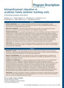
Fig. 2: Top of data entry sheet for CYTOS program. Data to be filled in include: Animal (equations for hair cell density will need to be changed, depending on species); Frequency of exposure (kHz or Hz); Duration of exposure (minutes, hours, days, weeks, months or years); Ear #; Age of animal (days, months or years); SPL of exposure (dB); Recovery after exposure (minutes, hours or years); Date when animal was terminated; SV Deg - Length of region(s) of stria vascularis degeneration. If a value greater than 0 is entered, a window opens in which to enter the beginning and ending % distance of the degeneration; Pieces [number of pieces (physical and mathematical) into which cell loss data were summarized]. Downward -pointing triangles indicate that there is a list of potential entries for that parameter. 4

Fig. 3: Partly filled out cell count sheet in the CYTOS program for ear 269L. Animal was exposed to a 0.5-kHz OBN at 120 dB SPL for 13 hours and recovered for 1 month prior to fixation. The cells in the table that are grayed out were done so by the CYTOS program based on the pattern code for that segment. Values for these cells are determined by the program using the total length of the OC, segment length and the turn in which segment is located.

Fig. 4: After the raw data are entered in the CYTOS program and proofread, pressing the 'calculate' button on the same page fills in the gray cells as shown here.

5

Fig. 5: Once all the data are recorded on the cell count sheet(s) in the CYTOS program, pressing the 'MSG TABLE' button produces a table of the % loss of IHCs and OHCs as a function of % distance from the

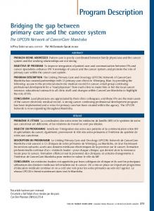
Fig. 6: Cytocochleogram and summary statistics for 269L. Boxes (top to bottom) summarize structural data as a function of cochlear location: StV DEG - extent of stria vascularis degeneration; ES condition of endolymphatic space; OC qualitative appearance of cells remaining in the OC; % missing hair cells - loss of IHCs (dashed line)and OHCs (solid line) and presence of total loss of all sensory and supporting cells (i.e., OC wipeout; solid vertical bar); and percentage loss of MNFs (peripheral processes of primary auditory neurons) and dieback distance (i.e., open bar - lateral to limbus; striped bar - within region of limbus; solid bar - medial to limbus).

6

Fig. 7: Cytocochleogram for 663R , a 19.2-year-old control chinchilla. There was a small region (0.3 mm) of stria vascularis degeneration (StV DEG) near the apex. The cell debris in the endolymphatic space is likely from the degenerated stria. This ear had 4.4% IHC loss and 20% OHC loss, distributed fairly evenly in the OC. There were four focal IHC lesions (i.e., 0.04, 0.03, 0.31, 0.03 mm in length), the largest of which had an adjacent degeneration of myelinated nerve fibers (MNF LOSS). The most prevalent pathological change in the supporting cells involved the pillars. The inner pillar (IP) bodies were out-of-place in the apical half of the OC whereas in most of the OC, outer pillar (OP) bodies were non-parallel to moderately buckled. Non-// adjacent OP bodies non-parallel; mod - moderately buckled OP bodies; sl - slightly buckled OP bodies. Data for the ES and OC boxes are recorded on a separate data sheet based on microscope findings and must be graphed by hand using a program such as PhotoShop.

Getting started The CYTOS program posted on Research Gate is in a zipped file. For windows users, it must be unzipped in 'C:\'. The chinchilla cochlea data base is posted as a zipped data set entitled 'Chinchilla cochlea data base'. Unzip the file and put it in a subdirectory entitled 'C:\CYTOS\data'. Summary tables of animals' age, exposure parameters etc. for all cochleae in the data base are posted as a pdf entitled 'Tables listing cochleae in Bohne's chinchilla data base'. The cochleae data base must be downloaded separately. 7

REFERENCES Bohne, BA (2012): The Plastic Embedding Technique for the Preparation of the Chinchilla Cochlea for Analysis by Phase Contrast Microscopy. Laboratory Manual, 7th Edition, Washington University Press. Bohne, BA, Harding, GW (1993): Combined organ of Corti/ modiolus technique for preparing mammalian cochleas for quantitative microscopy Hear. Res. 71:114-124. Bohne, BA, Harding, GW (2010): Analysis of the Normal and Damaged Inner Ear. Laboratory Manual, 5th edition, Washington University Press.

8