Jun 11, 1989 - AT&T Bell Laboratories. Murray Hill .... center point and calls the shape with the necessary arguments. It is usually ... shapes, and pic macros aren't general enough for the job, edges in pic drawings are clipped to a node's.
DAG— A Program that Draws Directed Graphs Revised June 11, 1989 E.R. Gansner S.C. North K.P. Vo AT&T Bell Laboratories Murray Hill, New Jersey 07974 ABSTRACT dag is a pic or POSTSCRIPT preprocessor that draws directed graphs. It works well on acyclic graphs and other graphs that can be drawn as hierarchies. Graph descriptions contain nodes, edges, and optional control statements. Here is a drawing of a graph from Forrester’s book, World Dynamics (Wright-Allen, Cambridge, MA, 1971). It took 2.1 CPU seconds on a VAX-8650 to make this drawing. S35
S24
S8
25
43
9
38
26
42
3
4
27
6
7
T24
S30
5
22
T35
23
11
31
37
36
40
21
32
19
41
2
17
33
34
S1
28
39
18
20
10
13
16
14
12
29
15
T30
T1
T8
I. Introduction Directed graphs have many applications in computing, such as describing data structures, finite automata, data flow, procedure calls, and software configuration dependencies. A picture is a good way to represent a directed graph. It is seldom easy to understand much about a graph from a list of edges, but with a picture one can quickly find individual nodes, groups of related nodes, and trace paths in the graph. The main obstacle is that it can be difficult and tedious to draw graphs by hand. dag is a program that draws directed graphs from edge lists. It does particularly well on acyclic graphs such as trees, DAGs, and other hierarchical graphs. It reads descriptions in a concise language and makes pic [K82] or POSTSCRIPT [A85] drawings. As a pic pre-processor, dag fits in the troff pipeline: dag file | pic | troff
II. Basics This section describes how to give a basic description of a graph as a list of edges. Figure 1 shows a dag description, and a reduced copy of the resulting picture.
Page 2 .GS 4 4 "5th Edition" "6th Edition"
"6th Edition" "PWB 1.0"; "Interdata" "Wollongong" "Mini Unix" "1 BSD" "LSX"; "Interdata" "7th Edition" "Unix/TS 3.0" "PWB 2.0"; "7th Edition" "8th Edition" "32V" "V7M" "Ultrix–11" "Xenix" "UniPlus+"; "V7M" "Ultrix–11"; "8th Edition" "9th Edition"; "1 BSD" "2 BSD"; "2 BSD" "2.8 BSD"; "2.8 BSD""2.9 BSD" "Ultrix–11"; "32V" "3 BSD"; "3 BSD" "4 BSD"; "4 BSD" "4.1 BSD"; "4.1 BSD""4.2 BSD" "2.8 BSD" "8th Edition"; "4.2 BSD""4.3 BSD" "Ultrix–32"; "PWB 1.0""PWB 1.2" "USG 1.0"; "PWB 1.2""PWB 2.0"; "USG 1.0""CB Unix 1" "USG 2.0"; "CB Unix 1" "CB Unix 2"; "CB Unix 2" "CB Unix 3"; "CB Unix 3" "Unix/TS++" "PDP–11 Sys V"; "USG 2.0""USG 3.0"; "USG 3.0""Unix/TS 3.0"; "PWB 2.0""Unix/TS 3.0"; "Unix/TS 1.0" "Unix/TS 3.0"; "Unix/TS 3.0" "TS 4.0"; "Unix/TS++" "TS 4.0"; "CB Unix 3" "TS 4.0"; "TS 4.0" "System V.0"; "System V.0" "System V.2"; "System V.2" "System V.3"; .GE
5th Edition
6th Edition
1 BSD
LSX
Wollongong
PWB 1.0
Mini Unix
Interdata
7th Edition
UniPlus+
PWB 2.0
Xenix
2 BSD
PWB 1.2
32V
Unix/TS 1.0
3 BSD
Unix/TS 3.0
4 BSD
V7M
Ultrix-11
2.9 BSD
4.2 BSD
Ultrix-32
USG 2.0
CB Unix 1
USG 3.0
CB Unix 2
CB Unix 3
Unix/TS++
4.1 BSD
2.8 BSD
USG 1.0
PDP-11 Sys V
TS 4.0
8th Edition
4.3 BSD
9th Edition
System V.0
System V.2
System V.3
Figure 1 Graph descriptions begin with .GS and end with .GE. (In other versions of Unix, dag recognizes GD instead of GS.) If the maximum width and height of the drawing are given on the GS line, the drawing is scaled appropriately. The drawing in Figure 1 has a 4 inch by 4 inch bounding box. A graph description is a list of semicolon-terminated statements. All the statements in Figure 1 are edge statements that name a tail node and a list of head nodes. Edges fan out from the tail node. The statement "5th Edition" "6th Edition" "PWB 1.0"; makes an edge from 5th Edition to 6th Edition, and another from 5th Edition to PWB 1.0. Because the syntax of edge statements is simple, graph descriptions can be generated from the output of other tools, such as cflow, profilers, or make utilities, without much effort. There is also a verbose form for edge statements: edge from "5th Edition" to "6th Edition", to "PWB 1.0"; The keywords edge, from, to, and commas are optional. Node names may be quoted to protect white space, punctuation, or dag keywords. As shown, dag places nodes in ranks so that edges point downward if possible. Nodes are ordered from left to right within ranks to reduce edge crossings and long edges. If there are cycles in the graph it is not possible for all edges to point downward, so some edges will be inverted. For instance, the following graph contains a cycle a→b → c→a, so the edge c→a points upward.
Page 3
a .GS edge from a to b; edge from b to c; edge from c to a; .GE
b
c
Figure 2 Edges that point backward can be made: b .GS backedge from a to b; edge from b to c; edge from c to a; .GE
c
a
Figure 3 Path statements create chains of edges. Here is a way to rewrite part of the description of Figure 1: path from "Unix/TS 1.0" to "Unix/TS 3.0" to "TS 4.0" to "System V.0"; Beginning a graph description with .GR instead of .GS makes edges point from left-to-right as shown in Figure 4.
Rosser
Newton
Birkhoff
Whitney
Ritchie
Veblen
Church
Kleene
Moore
Scott
Turing Figure 4
Page 4
A backpath is a chain of back-edges. backpath from Subaru to Honda to Ferrari;
III. Node Attributes This section explains how to control the way nodes are drawn. The node attributes are shape, size, label, pointsize of the label, and color. By default nodes are drawn as 1⁄2 ´´ by 3⁄4 ´´ ellipses labeled with the node name in 14-point type. The size may be increased to fit the label. draw nodes sets default attributes for nodes created afterward in a graph description; nodes already created are not affected. draw nodelist sets attributes of individual nodes. Nodes in the nodelist are created if they do not already exist. III.1 Node Shapes
The pre-defined shapes are Box, Square, Circle, Doublecircle, Ellipse, Diamond, and Plaintext. Shape names are capitalized to avoid conflict with pic keywords. Here is an example involving node shapes: edge draw draw edge
from a to b; ETA, Apollo, NeXT as Box; nodes as Plaintext; from x to y;
a and b are drawn as ellipses; ETA, Apollo, and NeXT as boxes; and x and y as Plaintext because Plaintext became the default before x and y were created. User-defined node shapes are created by writing pic macros or POSTSCRIPT procedures. Shapes have three arguments: the node label, width, and height. In a pic macro these are $1, $2, and $3. In a POSTSCRIPT procedure the arguments are passed on the stack. To draw a node, dag moves to its center point and calls the shape with the necessary arguments. It is usually convenient to define macros within the graph description in a block between .PS and .PE. The contents of this block are passed straight through dag and appear in the graphics code after the standard prologue but before any nodes or edges are drawn. There are two limitations on user-defined shapes. First, dag assumes height and width and independent. So if a user-defined shape has a fixed aspect ratio, fine-tuning may be needed to make the drawing look right. Second, because dag doesn’t know how to compute the boundary of user-defined shapes, and pic macros aren’t general enough for the job, edges in pic drawings are clipped to a node’s bounding rectangle. The second limitation does not apply to shapes written in POSTSCRIPT since the user also supplies a clipping procedure (see Appendix B). Figure 5 shows an example shape macro in pic. III.2 Node Labels
The default label of a node is its name. Another label can be set, which is particularly useful to allow distinct nodes to share a common label. draw "/usr/src/cmd" label "cmd"; draw "/usr/local/src/cmd" label "cmd"; III.3 Node Colors
Nodes may have color in POSTSCRIPT drawings. A color value is a string that is passed to the procedure dagsetcolor in the emitted POSTSCRIPT code. In the standard POSTSCRIPT prologue this procedure accepts a hue-saturation-brightness triple. Macros for common colors can be defined in a .PS/.PE block:
Page 5
.GS .PS define Triplecircle % [ circle rad .5 * $2; circle rad .475 * $2 at last circle.c; circle rad .45 * $2 at last circle.c; $1 at last circle.c; ]% .PE edge from 1 to 2; draw 1 as Triplecircle height 1 width 1; draw 2 as Circle height 1 width 1; .GE
1
2
Figure 5 .PS /red [.1 1 1] def .PE draw important_node color red; Other interpretations of color values may be implemented by redefining dagsetcolor and defining compatible node shapes. Appendix B explains how to make gray-scale shaded nodes this way.
IV. Edge Attributes This section explains how to control the way edges are drawn. The edge attributes are label, pointsize of the label, ink style, color, and weight. Attributes may be set when edges are created. draw edges sets default attributes for edges created afterward in the graph description. Previously created edges cannot be changed because unlike nodes, edges do not have identifiers. IV.1 Edge Labels
A label is a text string or fragment of executable graphics code drawn at the midpoint of an edge. Text labels are preferred. Graphics code is available for extreme cases, but it is discouraged because it is dependent on the target graphics language. Graphics code is enclosed in curly braces as shown below. edge from a to b label "x" ; edge from b to c label {circle rad .1}; Figure 6 is the description of a finite automaton with labeled edges and its picture. IV.2 Edge Weights
Edge weights or costs are integers. Increasing the weight of an edge makes dag try to shorten it. The default weight is 1; dag internally increases the weight of long edges to improve the drawing. In the Unix History graph of Figure 1, we might want to favor the edge "2 BSD" "2.8 BSD" over "4.1 BSD" "2.8 BSD". This suggests: edge from "2 BSD" to "2.8 BSD" weight 1000; It’s best to use large values to swamp the internal adjustment, otherwise a little experimenting with weights will probably be needed.
Page 6
.GR 6 draw nodes as Circle width .5 height .5; draw LR_0 LR_3 LR_4 LR_8 as Doublecircle width .5 height .5; draw edges pointsize 8; LR_0 LR_2 label "SS(B)"; LR_0 LR_1 label "SS(S)"; LR_1 LR_3 label "S($end)"; LR_2 LR_6 label "SS(b)"; LR_2 LR_5 label "SS(a)"; LR_2 LR_4 label "S(A)"; LR_5 LR_7 label "S(b)"; LR_5 LR_5 label "S(a)"; LR_6 LR_6 label "S(b)"; LR_6 LR_5 label "S(a)"; LR_7 LR_8 label "S(b)"; LR_7 LR_5 label "S(a)"; LR_8 LR_6 label "S(b)"; LR_8 LR_5 label "S(a)"; .GE
LR_1
S($end)
LR_3
SS(S) S(a)
LR_0 S(a)
LR_5
SS(B)
LR_7
S(b)
S(b)
SS(a)
LR_2
LR_8
S(a)
S(b)
S(A)
S(b)
LR_4 S(a)
LR_6
SS(b)
Figure 6 IV.3 Edge Styles
The graph description may name the ‘‘ink’’ or line style for edges: solid, dotted, dashed, or invis. edge from "2 BSD" to "2.8 BSD" dashed; Unfortunately troff does not have dotted or dashed splines so they appear as solid splines in pic output. IV.4 Edge Colors
Edge colors are much like node colors. edge from "2 BSD" to "2.8 BSD" color "[.2 1 1 ]"; draw edges "[.3 .5 .5]";
Page 7
V. Spacing Control Separate statements set the minimum spacing in inches between adjacent nodes or ranks. separate separate separate separate
nodes ranks ranks ranks
.75; 2; 2 exactly; 2 equally;
Because some drawings have edges that are almost horizontal and thus hard to read, dag may increase the separation between certain ranks to improve the drawing. When this happens, a side-effect is that ranks are not equally spaced. The adverb ‘‘equally’’ tells dag to maintain even spacing between ranks, which may be more aesthetically pleasing and readable. ‘‘exactly’’ inhibits the rank spacing adjustment. Another kind of spacing control is requested by putting the keyword fill on the GS line. This forces the drawing to fill the bounding box by increasing the node and rank separations. fill overrides ‘‘separate ranks exactly’’. For example: .GS 6 8 fill
VI. Rank Assignment Control The graph description may state that certain nodes should be placed on the minimum or maximum rank, or be kept as a group on the same rank. minimum rank root1 root2 root3; maximum rank leaf38 leaf39; same rank add sub mul div shift; Figure 7 is another drawing of Forrester’s World Dynamics graph. In this drawing, (1) source nodes S1, S8, S24, S30 and S35 are constrained to appear at the minimum rank, (2) target nodes T1, T8, T24, T30 and T35 are to appear at the maximum rank, and (3) all other nodes stay at the same ranks as in the drawing of the abstract.
S24
S8 25
S1
9 26
2 42
3
5
7
17
T8
16
21
18
S30 43
37
38 19
20
22 27
36
11
4
6
S35
15
10
40
13
14
41 39
12
33
28 29
34
31
32
23 T24
T35
T1
T30
Figure 7 Figure 8 illustrates how a time-line can be created with same rank statements. Forcing a group of nodes to be on the same rank can cause flat-edges, i.e., edges that point sideways instead of upward or downward. If possible, dag draws flat-edges from left to right. (This means that, as a side-effect, left-to-right order in a rank can be controlled by creating invisible flatedges.) Figure 9 shows a graph description in which the relative placements of nodes are completely specified. The edge crossing is unavoidable.
Page 8
1971
Thompson sh
1972
Ritchie cpp
1973 1974
SCCS
1975 1976
make
Mashey sh
Bourne sh
1977 1978
augmented make
1979
Csh
Form sh
build
1980
vi
1981 RCS
vsh
esh
etc. ksh
1983 8th ed. make
1984
Versioned files
1985
nmake mk
1986
future
emacs
1982
1987
Reiser cpp
fdelta
nmake+viewpaths extended directories
ksh-i
ncpp
n2make
Ansi cpp
Advanced Software Development Environment
Figure 8 If edges are ordered, dag automatically places head nodes on the same rank and creates invisible flat-edges. Figure 10 is a small part of a parse tree. Ordered edges are needed to correctly represent the grammar.
Page 9
.GS same rank 1 2; same rank 3 4; 1 4; 2 3; 1 2 invis; 3 4 invis; .GE
1
2
3
4
Figure 9
.GS ordered edge from "for–stmt" to "for" "var" "=" "expr1" "to" "expr2"; ordered edge from "expr1" to "left_op" "*" "right_op"; .GE
for-stmt
for
var
=
left_op
expr1
*
to
expr2
right_op
Figure 10 There are many other properties of a graph drawing that one might want to control, but it is difficult to build a good tool that achieves many, possibly conflicting, aesthetic goals. Users can exercise some control over node placement by setting edge weights and creating invisible edges. For finer control over drawings we suggest changing the drawing with a graphical editor or by modifying the generated code. There are no absolute restrictions on the graphs that dag can draw. Self-edges and multi-edges are allowed. For picture clarity, it’s best to avoid nodes with many incident edges. For instance, in procedure call graphs, it is a good idea to eliminate common library calls (e.g., stdio) before making the drawing. Removing these less interesting nodes both yields a more informative drawing and reduces run time.
VII. Drawing Algorithms dag has three main components: the parser, draw_dag, and the code generator. The parser is written in YACC. It constructs a graph of attributed nodes and edges in memory. The graph is passed to the drawing procedure draw_dag, which sets X and Y coordinates of nodes and spline control points of edges. The code generator traverses the attributed graph to emit target code in an obvious fashion. draw_dag is thus the heart of dag.
Page 10
To design algorithms for drawing graphs, we need to define what makes a good drawing. We have chosen three desirable properties for drawings of directed graphs: P1. The drawing should reveal the partial order implied by edges of the graph. Nodes are placed in ranks so that edges points downward. If the graph is not acyclic, cycles are broken by reversing edges. P2. The drawing should not be cluttered with irrelevance. For example, edge crossings are undesirable because they suggest a connection that is not really present in the underlying abstract graph. Edges also should not intersect nodes that are not their endpoints. P3. The drawing should reveal the relationships implied by edges by placing adjacent nodes in the graph close together. Unfortunately, these goals conflict. For instance, the placement of nodes in ranks may make it impossible to avoid edge crossings. Also, the minimization of edge-crossings in a layout is computationally intractable. So we are satisfied to find heuristics that run quickly and make good layouts in common cases. We sketch these techniques briefly as an aid to understanding the behavior of dag. draw_dag has four passes. The first pass finds an optimal rank assignment for the nodes, satisfying P1 and P3. The optimal rank assignment problem is to assign integer ranks to nodes such that the sum of the weighted edge lengths is minimized. The length of an edge here is taken as the difference in the ranks of its head and tail nodes. The optimal rank assignment problem can be formulated as an integer program. Because of its special characteristics the simplex method for linear programming can be used to solve these integer programs. However we have developed a combinatorial algorithm that finds the solution in a factor of O( E ) less time than the standard simplex algorithm and uses only O( E ) space. Following rank assignment, draw_dag creates dummy nodes where long edges cross ranks. The placement of dummy nodes determines edge crossings and is also an aid to drawing splines for long edges. Consequently, optimal rank assignment is important not only for drawing quality, but also to minimize the number of dummy nodes. This reduces edge crossing and improves the running time of subsequent passes that have a factor of O( V ) in their running time. The second pass orders nodes from left to right within ranks. This pass tries to reduce edge crossings (P2) subject to the constraints on node order implied by flat edges (P1). It is based on an iterative technique like that of [S81][R86]. The key improvements are a new weight function and local optimizations. We call the weight function the ‘‘generalized median’’; it produces less crossings by reducing the effects of widely spread nodes, and is inexpensive to compute. Informally, the generalized median of a node with respect to an adjacent rank is defined as follows. When the number of neighbors of a node in the concerned adjacent rank is odd, the generalized median is simply the median position of its neighbors. When the number of neighbors is even, the generalized median is in between the left and the right median positions. The exact value is tilted toward the side where neighbor nodes are more tightly packed. The generalized median heuristic (and other similar heuristics) tends to work better if the initial order of nodes is good. To enhance this condition, we apply transpositions of adjacent nodes to precondition the inputs to the generalized median method and to further optimize its solutions. The transposition heuristic can be viewed as a descent method to find local optima. The third pass assigns absolute coordinates to nodes, respecting the ordering determined by the previous pass (P3). The optimal assignment can be formulated as a set of linear constraints and an objective function involving absolute values. This can be transformed into a linear program by a standard technique that involves introducing extra variables. dag –O works this way. Since this pass is the bottleneck in draw_dag, we have developed a fast heuristic based on computation of the generalized median positions of adjacent nodes with additional local optimizations. The final pass finds the spline control points for edges. There are several cases to consider, including self-edges, edges between nodes on the same rank, adjacent ranks, or nonadjacent ranks,
Page 11
possibly in the presence of multi-edges. Short edges are easy to draw; we use a single B-spline [M85] that is shaped according to the number of parallel multi-edges being drawn. Long edges, or edges that have endpoints on nonadjacent ranks, are more difficult since they may pass near other nodes and change direction. The B-spline control points are chosen for • • •
smoothness, avoiding node intersections, and avoiding edge crossings.
The dummy nodes are created with a height a little larger than the highest non-dummy node in the same rank, and width usually twice the default node separation. This is big enough to make a spline inside the boundaries of the dummy node, if necessary. On the other hand, if there is space next to the dummy node, it is often preferable to encroach on it to draw a smoother spline. The edge drawing procedure in draw_dag visits each dummy node to choose its spline control points. If a straight line between the neighbors of the dummy node does not intersect any other node, nor change the order of edge crossings, then the dummy node is deleted (Figure 11a). This removes small bumps in the edges. Next, draw_dag aims the incident edges as close to the center of the dummy node box as possible, without intersecting adjacent nodes. draw_dag uses the points where the edges intersect the dummy node as spline control points. It also finds a third point to determine how the spline bends as it passes through the dummy node. If the intersection of the edges lies inside the dummy node (Figure 11b), draw_dag chooses it as the third control point. Otherwise, draw_dag tries to move the edges toward each other so they do intersect (Figure 11c) and again takes the intersection as the third control point. If the edges can’t be made to intersect, but the angle between them is acute, draw_dag can still make a smooth spline by choosing the midpoint of the opposite side. When the angle is obtuse, that is, the edges are close to being parallel, then it chooses the midpoint of the dummy node box. In the latter case the spline has two points of inflection as it passes through the dummy node, which is not as smooth as the other cases which have only one, but the extra turn is necessary when an edge makes a jog as it passes through a rank near other nodes (Figure 11d). Moving an edge may create an edge intersection near an incident real (non-dummy) node, as in Figure 11e. Such intersections are eliminated by sorting the incident edges according to the X coordinates of the other endpoints, and moving their nearby endpoints slightly (Figure 11f). Tables 1-3 show the performance of draw_dag using various node placement methods. The tables list the time spent in the three node placement passes: time spent on level (or rank) assignment t level , time spent ordering nodes within ranks to reduce edge crossings t cross , and time spent finding final coordinates t coord . The total time t total is the sum of these plus time spent in initialization and creating splines. The times were measured on a VAX-8650 under the 4.3BSD UNIX System and averaged over 5 runs to reduce statistical fluctuation. Times were measured on three graphs, the World Dynamics graph from the abstract of this paper and two procedure call graphs from C programs. World Dynamics has 48 nodes and 69 edges. The initial placement has 126 crossings. CallGraph-1 in Figure 12 has 38 nodes, 58 edges, and the initial placement has 128 crossings. CallGraph-2 in Figure 13 is dag’s call graph of 170 nodes and 258 edges. Its initial placement has 1170 crossings. We tried three algorithms for ordering of nodes within ranks: (1) gmedian is dag’s generalized median algorithm, (2) bcenter is the barycenter method described in [S81], and (3) rmedian is the ‘‘right median’’ [E86], which orders nodes using the position of the median neighbor when the number of neighbors is odd, and the right median neighbor otherwise. We also tried all three methods in combination with transposition of adjacent nodes. To simplify the comparison of relative performance, the iterative loop for minimizing edge crossing is set to terminate after exactly 20 iterations. In practice, the loop termination is determined by an adaptive parameter that depends on the convergent rate of a solution. Thus, for example, the total time for the World Dynamics graph using gmedian+ is slightly higher than it would be in an actual run. The experiments show that generalized median behaves well in a variety of test cases, and in about the same run-time as the other methods. All three methods improved by adding transposition, which seems well worth the extra computational expense. In Table 1, transposition reduced edge crossing by 30%.
Page 12
•
• • •
• •
(a)
(b)
(c)
(e)
(f)
• • •
(d)
Figure 11
_______________________________________________ _______________________________________________ World Dynamics Method n cross t level t crossing t coord t total _______________________________________________ gmedian 59 .06 .47 .56 1.18 _______________________________________________ _______________________________________________ bcenter 59 .06 .44 .47 1.08 rmedian 62 .05 .45 .51 1.11 _______________________________________________ _______________________________________________ gmedian+ 41 .06 1.30 .49 1.96 bcenter+ 43 .06 1.23 .50 1.88 _______________________________________________ rmedian+ 47 .05 1.25 .49 1.88 _______________________________________________ Table 1
Page 13
progen
scanner
look_ahead
quote_token
setbuf
put_one
range_walker
comment_scan
expreval
next_op
next_val
setblkval
tree_walker
mcprse
token_fetch
refblkval
dnfeval
tilde_token
unget_one
initsymtbl
atol
echo_of
mclex
setsymval
Mapblk
next_or
q_token
ret_token
unget_ch
refsymval
incrsymval
Mapsym
bhash
xmalloc
get_ch
ungetc
Figure 12. CallGraph-1. _______________________________________________ _______________________________________________ CallGraph-1 Method n t t t t cross level crossing coord total _______________________________________________ gmedian 12 .04 .38 .57 1.08 _______________________________________________ _______________________________________________ bcenter 10 .04 .44 .90 1.48 rmedian 14 .04 .43 .70 1.26 _______________________________________________ _______________________________________________ gmedian+ 11 .03 .73 .85 1.73 bcenter+ 11 .04 .77 .64 1.56 _______________________________________________ rmedian+ 11 .05 .89 .64 1.67 _______________________________________________ Table 2
hash
randstr
Page 14
Figure 13. CallGraph-2. ________________________________________________ ________________________________________________ CallGraph-2 Method n cross t level t crossing t coord t total ________________________________________________ gmedian 193 .50 2.87 2.91 6.52 ________________________________________________ ________________________________________________ bcenter 249 .53 2.73 2.82 6.36 rmedian 227 .53 2.96 3.07 6.84 ________________________________________________ ________________________________________________ gmedian+ 154 .51 8.11 3.32 12.23 bcenter+ 145 .52 8.21 3.05 12.04 ________________________________________________ rmedian+ 200 .50 8.35 3.75 12.86 ________________________________________________ Table 3
VIII. Conclusions dag is a practical tool for drawing directed graphs. We have favored ease of use over low-level drawing control, by providing a simple graph description language and a few well-tuned heuristics that produce good drawings quickly in common cases.
IX. References [A85]
Adobe Systems. Postscript Language Reference Manual, Addison-Wesley (1985).
[E85]
Eades, Peter, Brendan McKay, and Nicholas Wormald ‘‘An NP-Complete Crossing Number Problem for Bipartite Graphs,’’ University of Queensland, Dept. of Computer Science, Technical Report No. 60, St. Lucia, Queensland, 4067, Australia (1985).
[E86]
Eades, Peter, and David Kelly. ‘‘Heuristics for Drawing 2-Layered Networks,’’ ARS Combinatoria, 21:A, pp.89-98 (1986).
[K82]
Kernighan, Brian W. ‘‘PIC: A Language for Typesetting Graphics’’, Software: Practice and Experience 12:1, pp. 1-21 (1982).
Page 15
[M85]
Mortenson, Michael E. Geometric Modeling, Wiley and Sons (1985).
[R86]
Rowe, L. A., Michael Davis, Eli Messinger, Carl Meyer, Charles Spirakis, and Allen Tuan. ‘‘A Browser for Directed Graphs,’’ Software: Practice and Experience 17:1, pp. 61-76 (1986).
[S81]
Sugiyama, K.,S. Tagawa, and M. Toda. ‘‘Methods for Visual Understanding of Hierarchical System Structures’’, IEEE Transactions on Systems, Man, and Cybernetics SMC-11:2, pp. 109-125 (February 1981).
Page 16
Appendix A. DAG Syntax program
: ;
statement-list
statement-list
: ;
statement-list statement /* empty */
statement
: ;
draw-statement edge-statement control-statement
draw-statement : ;
draw node-list node-desc ; draw nodes node-desc ; draw edges edge-desc ;
node-list
: ;
node-list [,] node-name node-name
node-desc
: ;
node-desc-item node-desc node-desc-item
node-desc-item
: ;
width float height float pointsize integer label string label { drawing-code } as { drawing-code } as string color string
edge-statement
: ;
[ordered] [[back]edge from] node-name [to] head-list ; [back]path [from] node-name [to] head-list ;
head-list
;
head-list head head-list [,] [to] head /* empty */
head
: ;
node-name edge-desc node-name
edge-desc
: ;
edge-desc-item edge-desc edge-desc-item
Page 17
edge-desc-item
: ;
weight integer label string label { drawing-code } pointsize integer color string inkvalue
inkvalue
: ;
solid dashed dotted invis
control-statement : ;
separate sep-list ; minimum rank node-list ; maximum rank node-list ; same rank node-list ;
sep-list
: ;
sep-list sep-item /* empty */
sep-item
: ;
nodes ranks ranks ranks
node-name
: ;
string
float float float exactly float equally
A string is any sequence of non-whitespace, non-punctuation characters, or any quoted string that does not contain a newline. drawing-code is any sequence of characters containing balanced left and right curly braces.
Appendix B. POSTSCRIPT Interface dag –Tps generates POSTSCRIPT code. The drawing is in the default POSTSCRIPT coordinate system [A85]. Two procedures are needed to define a new node shape. The first draws the shape over the current point. It takes three arguments off the stack: the node width, height, and name. The second procedure computes where edges intersect the shape. Its arguments are the x and y dimensions of the shape, and a ray. The first point is the origin and the second point that defines the ray is always on the bounding box of the node when it is placed at ( 0 , 0 ). This procedure returns the point where the ray intersects the shape (or if it misses the shape, then the nearest point or at least the point on the bounding box that was passed as an argument). The argument points are always in the same quadrant. For some examples of shape-drawing procedures, examine the output of dag –Tps for definitions of procedures such as Ellipse and Ellipse_clip.
Page 18
Shaded nodes may be useful when color output is not available. Here is an example. .GR .PS /setdagcolor {/daggrayscale exch def} def /ShadedBox { /height exch def /width exch def /nodename exch def currentpoint 2 copy newpath moveto width –2 div height –2 div rmoveto width 0 rlineto 0 height rlineto width neg 0 rlineto closepath gsave daggrayscale setgray fill grestore stroke moveto nodename width .9 mul height .9 mul daglabel } def /ShadedBox_clip { Box_clip } def .PE draw nodes as ShadedBox; draw nodes color "1"; draw a color ".7"; draw b color ".9"; a b c; .GE setdagcolor is called before drawing a node or edge. The color value is emitted as POSTSCRIPT code which usually pushes something on the stack that setdagcolor consumes. For drawing shaded boxes, colors will be real values between 0 and 1, where 0 is black and 1 is white. Thus setdagcolor is redefined to store its argument it in the global variable daggrayscale where ShadedBox can find it later. In the definition of ShadedBox, the path of rectangle is created and then the sequence daggrayscale setgray fill shades its interior. The shading is done within gsave/grestore because we don’t want to shade the outline of the box itself, or its label. Since ShadedBox has the same boundary as Box, ShadedBox_clip is implemented by calling Box_clip.