damage identification with linear discriminant

DAMAGE IDENTIFICATION WITH LINEAR DISCRIMINANT OPERATORS

1

2

1

3

Charles R. Farrar , David A. Nix , Thomas A. Duffey , Phillip J. Cornwell , 4 Gerard C. Pardoen 1

Engineering Analysis Group, MS P946, Los Alamos National Laboratory, Los Alamos, NM, 87545 Computer Research and Application Group, MS B265, Los Alamos National Laboratory, Los Alamos, NM 87545 3 Dept. of Mechanical Engineering, Rose-Hulman Inst. of Tech., Terre Haute, IN, 47803 4 Dept. of Civil Engineering, Univ. of California-Irvine, Irvine, CA, 92717 2

ABSTRACT

This paper explores the application of statistical pattern recognition and machine learning techniques to vibrationbased damage detection. First, the damage detection process is described in terms of a problem in statistical pattern recognition. Next, a specific example of a statistical-pattern-recognition-based damage detection process using a linear discriminant operator, “Fisher’s Discriminant”, is applied to the problem of identifying structural damage in a physical system. Accelerometer time histories are recorded from sensors attached to the system as that system is excited using a measured input. Linear Prediction Coding (LPC) coefficients are utilized to convert the accelerometer time-series data into multidimensional samples representing the resonances of the system during a brief segment of the time series. Fisher’s discriminant is then used to find the linear projection of the LPC data distributions that best separates data from undamaged and damaged systems. The method is applied to data from concrete bridge columns as the columns are progressively damaged. For this case, the method captures a clear distinction between undamaged and damaged vibration profiles. Further, the method assigns a probability of damage that can be used to rank systems in order of priority for inspection. 1. INTRODUCTION Damage detection as determined from changes in the vibration characteristics of a system has been a popular research topic for the last thirty years. Numerous papers have appeared at past IMAC conferences related to this topic, and this subject was the theme for IMAC XV. Doebling, et al. (1996) [1], present a review of vibrationbased damage identification methods. Few of the

references cited in this review take a statistical approach to the damage detection process. However, because all vibration-based damage detection processes rely on experimental data with their inherent uncertainties, statistical analysis procedures are necessary if one is to state in any quantifiable manner that changes in the vibration properties of a structure are indicative of damage as opposed to test-to-test variability. This paper will first pose the general problem of the vibration-based damage detection process in the context of a problem in statistical pattern recognition. Next, a tool that has been developed for statistical pattern recognition, specifically a linear discriminant operator referred to as “Fisher’s Discriminant,” will then be applied to vibration data from undamaged and damaged structures to demonstrate this process. The University of California, Irvine (UCI) has a contract with CALTRANS to perform static, cyclic tests to failure on seismically retrofitted, reinforced-concrete bridge columns. This project is under the direction of Prof. Gerry Pardoen at UCI. With funds obtained through Los Alamos National Laboratory’s (LANL) University of California interaction office, staff from the LANL’s Engineering Analysis Group and a faculty member from the Mechanical Eng. Dept. at Rose-Hulman Institute of Technology were able to perform numerous experimental modal analyses on the columns. These modal tests were performed at stages during the static load cycle testing when various amounts of damage had been accumulated in the columns. These tests and the associated data obtained will be used to demonstrate a statistical pattern recognition process of vibration-based damage detection.

IMPLEMENTATION OF STRUCTURAL DAMAGE DETECTION 1. OPERATIONAL EVALUATION A. Operational and Environmental conditions B. Constraints on data acquisition

2. DATA ACQUISITION AND CLEANSING A. Define data to be acquired B. Define data to be used (or not used) in the feature selection What Types and How Much Data Should be Acquired Where Should Sensors be Placed Define the Data Acquisition, Storage and Transmittal

How Often Should Data be Acquired A. Only after extreme events B. Periodic intervals C. Continuous

Data Normalization Procedures A. Level of input B. Temporal

Sources of Variability A. Changing environmental/testing/data reduction conditions B. Unit-to-Unit Variability

Feedback from Model Development

Feedback from Feature Selection

3. FEATURE SELECTION A. What features of the data are best for damage detection B. Statistical distribution of features C. Data condensation Basis for Feature Selection A. Numerical Analysis B. Past Experience C. Component Testing Feedback from Model Development

Sources of Variability

Physical Models for Feature Selection A. Linear vs Nonlinear B. Purely Experimental or Analytical/Experimental

4. STATISTICAL MODEL DEVELOPMENT A. Data available from undamaged and damaged system B. Data available only from undamaged or current system Is it damaged or undamaged? (group classification) (Identification of outliers)

Where is the damage located? (regression analysis)

What is the extent of damage? (regression analysis) Remaining useful life of the system

What type of damage is it? (regression analysis) Incorrect diagnosis of damage False-positive results False-negative results

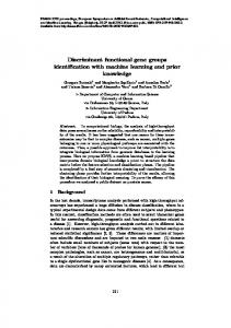
Fig. 1 Flow chart for implementing a structural damage detection program. 2. THE DAMAGE DETECTION PROCESS In the context of statistical pattern recognition the process of vibration-based damage detection can be broken down into four parts as summarized in Fig. 1. The topics summarized in this flow chart are briefly discussed below. 2.1. Operational Evaluation An operational structure is defined to be one that can perform or is performing its intended function. Operational structures are often geometrically complex and may be too large to test in a laboratory. Also, the boundary conditions associated with such in situ structures are often not well known. Finally, the environment and the test conditions associated with an operational structure are often changing and can have a significant impact on the measured structural response.

Operational evaluation answers two questions in the implementation of a structural health monitoring system:

1. 2.

What are the conditions, both operational and environmental, under which the system to be monitored functions; and What are the limitations on acquiring data in the operational environment.

Operational evaluation begins to set the limitations on what will be monitored and how the monitoring will be accomplished. This evaluation starts to tailor the damage detection process to features that are unique to the system being monitored and tries to take advantage of unique features of the damage that is to be detected. 2. 2. Data Acquisition and Cleansing The data acquisition portion of the structural health monitoring process involves selecting the types of sensors to be used, the location where the sensors should be placed, the number of sensors to be used, and the data acquisition/storage/transmittal hardware. Again, this

process will be application specific. Economic considerations will play a major role in making these decisions. Another consideration is how often the data should be collected. For earthquake applications it may be prudent to collect data immediately before and at periodic intervals after a large event. If fatigue crack growth is the failure mode of concern, it may be necessary to collect data almost continuously at relatively short time intervals. Because the data can be measured under different conditions, the ability to normalize the data becomes very important to the damage detection process. One of the most common normalizing procedures is to normalize the measured responses by the measured inputs. When environmental variability is an issue, the need can arise to normalize the data in some temporal fashion to facilitate the comparison of data measured at similar times of an environmental cycle. Sources of variability in the data acquisition process should be identified and minimized to the extent possible. In general, all sources of variability can not be eliminated. Therefore, it will be necessary to make the appropriate measurements such that these sources can be statistically quantified. Data cleansing is the process of selectively choosing data to accept for, or reject from, the feature selection process. The data cleansing process is usually based on knowledge gained by individuals directly involved with the data acquisition. Finally, is should be noted that the data acquisition and cleansing portion of a structural health-monitoring process should not be static. Insight gained from the feature selection process and the statistical model development process will provide information regarding changes that can improve the data acquisition process. 2. 3. Feature Selection The area of the structural damage detection process that receives the most attention in the technical literature is the identification of data features that allows one to distinguish between the undamaged and damaged structure. Inherent in this feature selection process is the condensation of the data. Probably the most common features that are used in vibration-based damage detection, and that represent a significant amount of data condensation from the actual measured quantities, are modal properties and subsequent properties derived from them such as mode shape curvature. However, the best features for damage detection are typically application specific. A variety of methods are employed to identify features for damage detection. Past experience with measured data from a system, particularly if damaging events have been previously observed for that system, is often the basis for feature selection. Numerical simulation of the damaged system’s response to simulated inputs is another means of

identifying features for damage detection. The application of engineered flaws, similar to ones expected in actual operating conditions, to specimens can identify parameters that are sensitive to the expected damage. Damage accumulation testing, during which significant structural components of the system under study are subjected to a realistic accumulation of damage, can also be used to identify appropriate features. Fitting linear or nonlinear, physical-based or non-physical-based models of the structural response to measured data can also help identify damage-sensitive features. The operational implementation and diagnostic measurement technologies needed to perform structural health monitoring typically produce a large amount of data. A condensation of the data is advantageous and necessary particularly if comparisons of many data sets over the lifetime of the structure are envisioned. Also, because data may be acquired from a structure over an extended period of time and in an operational environment, robust data reduction techniques must be developed to retain sensitivity of the chosen features to the structural changes of interest in the presence of environmental noise. To further aid in the recording of quality data and feature extraction needed to perform structural damage detection process, the statistical significance of the data changes should be characterized and used in the condensation process. 2. 4. Statistical Model Development The portion of the structural health monitoring process that has received the least attention in the technical literature is the development of statistical models to enhance the damage detection process. Statistical model development is concerned with the implementation of the algorithms to operate on the extracted features and unambiguously determine the damage state of the structure. The algorithms used in statistical model development usually fall into three categories and will depend on the availability of data from both an undamaged and damaged structure. The first category is group classification, that is, placement of the data into respective “undamaged” or “damaged” categories. Analysis of outliers is the second type of algorithm. When data from a damaged structure are not available for comparison, do the observed features indicate a significant change from the previously observed features that can not be explained by extrapolation of the feature distribution. The third category is regression analysis. This analysis refers to the process of correlating data features with particular types, locations or extents of damage. All three algorithm categories analyze statistical distributions of the measured or derived features to enhance the damage detection process. The damage state of the structure is usually described as a four-step process that answers the following questions at each step, Rytter (1993) [2]: 1. Is there damage in the structure (existence)?; 2. Where is the damage in the structure (location)?; 3. How severe is the damage (extent)?; and 4. How much useful life remains in the structure (prediction)? The steps in the process also represent increasing knowledge of the damage state.

Structural dynamics techniques are most useful for the first two steps. Analytical dynamics techniques are usually needed to answer the question associated with step three. The answer to the step four question is the most elusive and requires material constitutive information.

24” (61 cm) sq. Cylcic Static Load 18” (45.7 cm) 9” (22.9 cm)

A fifth category for statistical model development is to determine the type of damage present. This process usually requires that data from the specific types of damage are available to be correlated with the observed features. Finally, an important part of the statistical model development process is the testing of these models on actual data to establish the sensitivity of the damage detection and to study the possibility of false indications of damage. False indications of damage fall into two categories: 1.) False-positive damage indication (indication of damage when none is present), and 2). False-negative damage indications (no indication of damage when damage is present). Although the second category is usually very detrimental to the damage detection, false-positive readings can also erode confidence in the damage detection process. This paper will now summarize the application of methods from statistical pattern recognition and machine learning to the vibration-based damage detection problem. A damage detection experiment performed on concrete bridge columns will be described in terms of the statistical-patternrecognition damage-detection paradigm that has just been summarized.

136” (345 cm)

36” (91 cm) dia.

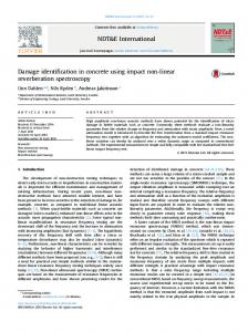
3. TEST STRUCTURE GEOMETRY The test structures consisted of two 24-in-dia (61-cm-dia) concrete bridge columns that were subsequently retrofitted to 36-in-dia (91-cm-dia) columns. Figure 2 shows the test structure geometry.The first column tested, labeled Column 3, was retrofitted by placing forms around the existing column and placing additional concrete within the form. The second column, labeled Column 2, was extended to the 36in-diameter by spraying concrete in a process referred to as shotcreting. The shotcreted column was then finished with a trowel to obtain the circular cross-section. The 36-in-dia. portions of both columns were 136 in. (345 cm) in length. The columns were cast on top of a 56-in-sq. (142-cm-sq.) concrete foundation that was 25-in-high (63.5cm-high). A 24-in-sq. concrete block that had been cast integrally with the column extends 18-in. (46-cm) above the top of the 36-in-dia. portion of the column. This block was used to attach the hydraulic actuator to the columns for quasi-static cyclic testing and to attach the electro-magnetic shaker used for the experimental modal analyses. As is typical of actual retrofits in the field, a 1.5-in-gap (3.8-cmgap) was left between the top of the foundation and the bottom of retrofit jacket. Therefore, the longitudinal reinforcement in the retrofitted portion of the column did not extend into the foundation. The concrete foundation was

1.5” (3.8 cm) 24” (61 cm) dia 56” (142 cm) sq

25.0” (63.5 cm)

Fig. 2 Column Dimensions bolted to the 2-ft-thick (0.61-m-thick) testing floor in the UCI laboratory during both the static cyclic tests and the experimental modal analyses. The structures were not moved once testing was initiated. The columns were constructed by first placing the th foundations on July 18 , 1997. Then the 24-in-diameter th columns were placed on August 19 and the retrofits were th added on September 19 . Corresponding portions of both test structures were constructed from the same batch of concrete. The only measured material property for these columns was the 28-day ultimate strength of the concrete and the test day ultimate strength. The 28-day ultimate strength of foundations was 4600 psi (32 MPa). Test day ultimate strength was not measured for the foundations. The 24-in-dia. Columns’ 28-day ultimate strength was 4300 psi (30 MPa) and the test day ultimate strength was 4800 psi (33 MPa). The 28-day-ultimate strength of the retrofit portion of the structures was 5200 psi (36 MPa). On test day the strength of the retrofit concrete was found to be 4900 psi (34 MPa).

Within the 24-in-dia initial column reinforcement consisted of an inner circle of 10 #6 (3/4-in-dia, 19-mm-dia) longitudinal rebars with a yield strength of 74.9 ksi (516 MPa). These bars were enclosed by a spiral cage of #2 (1/4-in-dia, 13.5mm-dia) rebar having a yield strength of 30 ksi (207 MPa) and spaced at a 7-in pitch (18 cm). Two-inch-cover (5- cmcover) was provided for the spiral reinforcement. The retrofit jacket had 16 #8 (1-in-dia, 25-mm-dia) longitudinal rebars with a yield strength of 60 ksi (414 MPa). These bars were enclosed by a spiral cage of #6 rebar spaced at a 6-in pitch (15 cm). The spiral steel also had a yield strength of 60 ksi. Again, 2-in.-cover was provided for this reinforcement. Lapsplices 17-in (43-cm) in length were used to connect the longitudinal reinforcement of the existing 24-in column to the foundation. 4. QUASI - STATIC LOADING Prior to applying lateral loads, an axial load of 90 kips (400 kN) was applied to simulate dead loads that an actual column would experience. A steel beam was placed on top of the column. Vertical steel rods, fastened to the laboratory floor, were tensioned by jacking against the steel beam that, in turn, applied a compressive load to the column. An hydraulic actuator was used to apply lateral load to the top of the column in a cyclic manner. The loads were first applied in a force-controlled manner to produce lateral deformations at the top of the column corresponding to 0.25∆yT, 0.5∆yT, 0.75∆yT and ∆yT. Here ∆yT is the lateral deformation at the top of the column corresponding to the theoretical first yield of the longitudinal reinforcement. The structure was cycled three times at each of these load levels. Based on the observed response, a lateral deformation corresponding the actual first yield, ∆y, was calculated and the structure was cycled three times in a displacementcontrolled manner to that deformation level. Next, the loading was applied in a displacement-controlled manner, again in sets of three cycles, at displacements corresponding to 1.5∆y, 2.0∆y, 2.5∆y, etc. until the ultimate capacity of the column was reached. Load deformation curves for Column 3 are shown in Fig 3. This manner of loading put incremental and quantifiable damage into the structures. The axial load was applied during all static tests. 5. DYNAMIC EXCITATION For the experimental modal analyses the excitation was provided by an APS electro-magnetic shaker mounted offaxis at the top of the structure. The shaker rested on a steel plate attached to the concrete column. Horizontal load was transferred from the shaker to the structure through a friction connection between the supports of the shaker and the steel plate. This force was measured with an accelerometer 2 mounted to the sliding mass (0.18 lb-s /in (31 Kg)) of the shaker. A 0 - 400 Hz uniform random signal was sent from a source module in the data acquisition system to the shaker

Fig. 3 Load –displacement curves for the cast-in-place column. but feedback from the column and the dynamics of the mounting plate produced an input signal that was not uniform over the specified frequency range. Fig. 4 shows a typical input power spectrum. The same level of excitation was used in all tests except for one at twice this nominal level that was performed as a linearity check. 6. OPERATIONAL EVALUATION Because the structure being tested was a laboratory specimen, operational evaluation was not conducted in a manner that would typically be applied to an in situ structure. However, the vibration tests were not the primary purpose of this investigation. Therefore, compromises had to be made regarding the manner in which the vibration tests were conducted. The primary compromise was associated with the mounting of the shaker. These compromises are analogous to operational constraints that may occur with in situ structures. Environmental variability was not considered an issue because these tests were conducted in a laboratory setting. The available measurement hardware and software placed the only constraints on the data acquisition process. 7. DATA ACQUISITION AND CLEANSING Forty accelerometers were mounted on the structure as shown in Fig. 5. These locations were selected based on the initial desire to measure the global bending, axial and torsional modes of the column. Note that locations 2, 39 and 40 had a nominal sensitivity of 10mV/g and were not sensitive enough for the measurements being made. As part of the data cleansing process, data from these channels were not used in subsequent portions of the damage detection process. Locations 33, 34, 35, 36, and 37 were accelerometers with a nominal sensitivity of 100mV/g. All other channels had accelerometers with a nominal sensitivity of 1V/g. During the test on the shotcrete column (column 2) the accelerometer at location 23 had to be replaced. All calibration factors were entered into the data acquisition system prior to the measurements. A calibration

Z

Spectral Function: PSD Ref −− Display Function: SISO

30” (76.2 cm)

−6

10

36, 37(load) 20

35

−7

10

19 MAG

−8

10

15.0” (38.1 cm) 40

21

34

17

33

18

32

14

31

15

30

11

29

12

28

8

27

22.67” (57.6 cm)

−9

10

16 −10

10

0

50

100

150

200 Freq (Hz)

250

300

350

400

39

22.67” (57.6 cm)

Primary Data, File=test0.mat, Reference DOF: 1 Secondary Data, File=testol.mat, Reference DOF: 1

13

Fig. 4 Input Power Spectra. The solid line corresponds to a test on an undamaged column without preload and the dashed line corresponds to a subsequent test when preload was applied. factor of 1.0 was entered for the accelerometer that monitored the sliding mass on the shaker.

38

10

2

7

Data acquisition parameters were specified such that frequency response functions (FRFs), input and response power spectra, cross-power spectra and coherence functions in the range of 0-400 Hz could be measured. Each spectrum was calculated from 30 averages of 2-s-duration time-histories discretized with 2048 points. These sampling parameters produced a frequency resolution of 0.5 Hz. Hanning windows were applied to all measured timehistories prior to the calculation of spectral quantities. A second set of measurements was acquired from 8-sduration time-histories discretized with 8192 points. Only one average was measured. A uniform window was specified for these data, as the intent was to measure a time history only. 8. FEATURE SELECTION The vibration response of the concrete columns was measured as previously described. Typically, systematic differences between time series from the undamaged and

22.67” (57.6 cm) 1

9

Data were sampled and processed with a Hewlett-Packard (HP) 3566A dynamic data acquisition system. This system includes a model 35650 mainframe, 35653A source module used to drive the shaker, five 35653A 8-channel input modules which provided power for accelerometers and performed the analog to digital conversion of accelerometer signals, and a 35651C signal processing module that performed the needed Fast Fourier Transform calculations. A Toshiba Tecra 700CT Laptop was used for data storage and as a platform for the HP software that controls the data acquisition system.

22.67” (57.6 cm)

26

5

25

4

22.67” (57.6 cm) 23

6

24 36” (91.4 cm) dia

3

22.67” (57.6 cm) 22

X

Fig. 5 Accelerometer locations and coordinate system for modal testing. Accelerometers 3, 6, 9, 12, 15, 18, 21, 22, 24, 26, 28, 30, 32, and 34 are mounted in the –y direction. damaged structures are nearly impossible to detect by eye. Therefore, other features of the measured data must be examined for damage detection. Originally, damage detection features were to be based on common modal properties as have been done in many previous studies. However, the feedback from the structure and mounting system to the shaker produced an input that did not have a uniform power spectrum over the frequency range of interest as previously discussed. This input form coupled with the nonlinear response observed at higher levels of damage made it extremely difficult to track changing modal properties through the various levels of damage. Therefore, other features were sought for the damage detection process.

The alternate features were selected based on previous experience from speech pattern recognition where autoregressive models have been used to estimate the transfer function of the human vocal track [3]. The time series were modeled using a common method of auto-regressive estimation also referred to as Linear Predictive Coding (LPC) [4]. The LPC algorithm is an Nth-order model that attempts to model the current point in a time series, s’(n) , as a linear combination of the previous N points. That is

maximally discriminates the {xA}’s from the {xB}’s. That is, it defines a linear projection {w} such that y = {w}T{x}

(2)

produces a scalar projection, y, of the multidimensional space onto which the distribution of {xA}’s is as distinct as possible from the distribution of {xB}’s. Once this projection is determined from previous samples of {xA}’s and {xB}’s it can be used to provide the relative probability that a novel sample {x} was generated by process A or B.

N

s ' (n ) =

∑ a s ( n − i) i

(1)

i =1

Third-order LPC models were developed for each column using 512-point windows with 97% overlap resulting in 480 samples of the ai’s. Over these segments of the time series the ai’s that best model the time series in a least squares sense are used as features that are assumed to be representative of the system’s dynamic response during those samples. Hanning windows were applied to these data prior to the estimate of the coefficients. These models were developed with data from sensors 3 and 21 (Fig. 5). Sensor 3 was located close to the damage, but because of the test configuration this sensor was not expected to experience large amplitude response as it primarily measures torsional motion of the structure near its fixed end. Sensor 21 was located farther from the damage and experienced some of the largest amplitude response as it primarily measured the bending response at the free end of this cantilever structure.

In determining {w}, it is not sufficient to simply consider the single dimension in which the means of the NA samples of {xA}’s and NB samples of {xB}’s, {µa} and {µb}, defined as

∑

{µ A }=

∑

1 {x A } and {µ B }= 1 {x B } (3) NB NA are farthest apart. For this case one would determine the projection {w} that maximizes the scalar quantity µA – µΒ where this difference is defined as µ A − µ B = {w}T ({µ A }− {µ B })

Such a projection does not account for the within-class scatter, that is, the width of each distribution in each dimension is not taken into account. The within-class scatter of the y data for class k can be described by the within-class covariance, sk2, where s 2k =

∑ (y

− µk ) , 2

n

Over a time series, many overlapping “windows'' give rise to LPC coefficient vectors, which become the multidimensional data samples to be analyzed in the statistical model development portion of the damage detection process. While the overlapping of windows provides a smoother estimate of the features’ changes over time, samples that result from overlapping windows will not be independent.

µk = {w}T{µk}, and

Normalization of the data was not attempted because these tests were conducted in a laboratory environment where the input could be applied in a very controlled manner. Other considerations that led to the decision not to normalize the data included the consideration that environmental and testto-test variability was negligible, damage was introduced in discrete increments, and it was assumed that the vibration levels were such that the physical condition of the test structures did not change during the dynamic tests.

F({w}) =

8. STATISTICAL MODEL DEVELOPMENT: FISHER’S DISCRIMINANT Consider two data generation processes A and B, with independent multi-dimensional samples {x} being generated by both processes. Assuming A and B have some systematic difference in the samples that they generate, Fisher's discriminant [5,6] represents the optimal linear projection of the multidimensional sample space that

(4)

(5)

n∈k

yn is obtained from Eq. 2, (6)

the total within-class scatter of the data from all samples of {x} (those generated by process A and B) is the sum of all sk2. Thus, the Fisher discriminant maximizes the function F({w}), which is the distance between the means of the transformed distributions, normalized by the total withinclass covariance:

(µA − µB )2 s 2A + s 2B

.

(7)

Using Eqs. 2 and 5 and the definition of a multi-dimensional sample mean given by Eq. 3, Equation 7 can be rewritten explicitly in terms of {w} as

{w}T [Sb ]{w} , {w}T [Sw ]{w}

(8)

[Sb ] = ({µB }− {µA })T ({µB }− {µA })

(9)

F({w}) = where

is the between-class covariance matrix, and

( x A }− {µ A }) [s w ] = ∑ ({x A }− {µ A }){ ( x B }− {µ B })T + ∑ ({x B }− {µ B }){

T

(10)

is the total within-class covariance matrix and the summations in Eq. 10 are over the available samples of {xA} and {xB}, respectively. To maximize F({w}), the derivative of F with respect to {w} is set equal to zero, yielding

({w} [S ]{w})[S T

b

w

]{w} = ({w}T [Sw ]{w})[Sb ]{w} .

(11)

The magnitude of {w} is not of concern, only its direction, therefore the scalar quantities

[({w} [S ]{w})] and ({w} [S T

T

b

w

]{w})

are replaced with arbitrary α and β, respectively. After rearrangement and multiplication by [Sw]-1 (note that because [Sw] is a covariance matrix, [Sw] is invertible), the following relation is obtained

[Sw ]−1[Sb ]{w} = α {w}.

(12) β Thus, with standard numerical methods {w} is found as an eigenvector of [Sw]-1 [Sb]. Once the data have been projected down onto the scalar y dimension, the distribution of yA and yB points can be described by an appropriate probability density function. Since it was originally assumed that {x} was a multidimensional random variable, then y = {w}T{x} is a sum of random variables and the central limit theorem is invoked to justify modeling yA and yB with Gaussian density functions. T

Novel data {xnew} can be projected to get ynew = {w} {xnew} and the likelihood, p, of ynew with respect to the Gaussian for class A and the Gaussian for class B can be determined. The probability that ynew was generated by class A can be obtained by integrating over a small region of the likelihood function:

(

)

P y new A =

∫p

A

(y new )dy .

(13)

∆y

Because P(A I ynew) is of interest, and

(

)

(

)

P B y new = 1 − P A y new ,

(14)

if A and B are mutually exclusive, Bayes' rule can be used to obtain

(

) P(y new( A )P)(A ) . P y new

P A y new =

(15)

where the denominator is typically ignored when P(ynew) is uniform (or unknown) and P(A) is the prior probability (i.e., relative frequency) of Class A vs. Class B. In the case where class A is ``undamaged'' and class B is ``damaged,'' a probability of a damaged system having produced a given observed sample {xnew} can now be estimated. 9. APPLICATION OF FISHER’S DISCRIMINANT TO CONCRETE COLUMN DATA Fisher's discriminant was defined using data from the vibration tests conducted on the undamaged columns and from the vibration tests conducted after the first level of damage corresponding to initial yielding of the steel reinforcement. Subsequent damage levels were then identified based on this same Fisher projection. As illustrated in Fig. 6, when Fisher’s discriminant is applied to data from both sensors on either column, there is statistically significant separation between the LPC coefficients for the undamaged cases and damage level 1 cases (solid and dashed Gaussian density functions). Also plotted are the results of using the previously determined Fisher projection to project many samples of data from increasingly greater levels of damage into this space. While increasing damage is not necessarily related to increasing Fisher coordinate, all damaged cases have a profile significantly different from that of the undamaged case. Higher-order LPC models and different size data windows produced similar results. 10. CONCLUSIONS A statistical-pattern-recognition paradigm has been proposed for the general problem of structural damage detection. This paradigm breaks the process of damage detection into the four tasks of operational evaluation, data acquisition and cleansing, feature selection, and statistical model development. A structural damage detection study of concrete columns subjected to quasi-static cyclic loading to failure is then posed in terms of this paradigm. A well-developed procedure for group classification, the linear discriminant operator referred to as “Fisher’s Discriminant”, was introduced for application to vibrationbased damage detection. This procedure requires data to be available from both the undamaged and damaged structures. Other statistical models that identify outliers can be used when data are available only from the undamaged structure. The results of this study indicate a strong potential for using linear discriminant operators for level 1 damage identification (is it damaged?). These methods do not simply classify incoming data as having been produced by “undamaged'' or “damaged'' systems. They assign a probability of damage that can be used to rank systems in order of priority for inspection. An attractive attribute of this statistical model is that it was applied to features obtained from response data only. The results obtained suggest the extension of this model to applications where structures are

subjected to ambient vibration from sources such as traffic or wind excitation.

Fig. 6 Distribution of LPC-generated feature vectors projected onto the Fisher coordinate. Solid horizontal lines represent two-standard deviation widths of the distributions for higher damage levels.

The results of this study also suggest that if one or more common forms of damage occur, it may be possible to not only determine that a system is damaged but to determine which form of damage has occurred. Additional data is required to explore this possibility. Another attractive feature of the linear discriminant operator that was not fully explored during this investigation is its ability to combine data from various types of sensors. This feature will become particularly attractive when monitoring structures that experience significant variations in their dynamic response resulting from changing environmental and operating conditions. Further analyses are also required to demonstrate the ability of the linear discriminant operator to avoid false-positive indications of damage. However, multiple samples of data from the undamaged columns were not measured. All data used in this study and a report summarizing the vibration testing are available at:

The authors would like to express their appreciation to Mr. Tim Leary at CALTRANS who allowed us to use his test structures for this investigation. 12. REFERENCES 1.

2.

3.

http://esaea-www.esa.lanl.gov/damage_id 4. 11. ACKNOWLEDGMENTS Funding for this research was provided by the Department of Energy through the Los Alamos National Laboratory’s University of California Interaction Office and the Department of Energy’s Enhanced Surveillance Program.

5.

Doebling, S.W., C.R. Farrar, M.B. Prime, and D.W. Shevitz (1996), “Damage Identification and Health Monitoring of Structural and Mechanical Systems from Changes in their Vibration Characteristics: A Literature Review”, LA-13070-MS, Los Alamos National Laboratory, Los Alamos, NM. Rytter, A. (1993) “Vibration Based Inspection of Civil Engineering Structures,” Doctoral Dissertation, Department of Building Technology and Structural Engineering, University of Aalborg, Aalborg, Denmark Morgan, D. P. and C. L. Scofield (1992) Neural Networks and Speech Pattern Processing, Kluwer Academic Publishers, Boston, MA. Rabiner, L.P. and R.W. Shafer (1978), Digital Processing of Speech Signals, Prentice-Hall, Inc., Englewood Cliffs, NJ. Fisher, R.A. (1936), “The Use of Multiple measurements in Taxonomic Problems”, Ann. Eugenics, Vol. 7, Part II, pp. 179-188.

6.

Bishop, C. M. (1995) Neural Networks for Pattern Recognition, Oxford University Press, Oxford, UK.