1
Data-dependent Hashing Based on p-Stable Distribution Xiao Bai, Haichuan Yang, Jun Zhou, Peng Ren and Jian Cheng
Abstract—The p-stable distribution is traditionally used for data-independent hashing. In this paper, we describe how to perform data-dependent hashing based on p-stable distribution. We commence by formulating the Euclidean distance preserving property in terms of variance estimation. Based on this property, we develop a projection method which maps the original data to arbitrary dimensional vectors. Each projection vector is a linear combination of multiple random vectors subject to p-stable distribution, in which the weights for the linear combination are learned based on the training data. An orthogonal matrix is then learned data-dependently for minimizing the thresholding error in quantization. Combining the projection method and the orthogonal matrix, we develop an unsupervised hashing scheme which preserves the Euclidean distance. Compared with data-independent hashing methods, our method takes the data distribution into consideration and gives more accurate hashing results with compact hash codes. Different from many datadependent hashing methods, our method accommodates multiple hash tables and is not restricted by the number of hash functions. To extend our method to a supervised scenario, we incorporate a supervised label propagation scheme into the proposed projection method. This results in a supervised hashing scheme which preserves semantic similarity of data. Experimental results show that our methods have outperformed several state-of-the-art hashing approaches in both effectiveness and efficiency.
I. I NTRODUCTION The volume of image data has been increasing dramatically every year. The big data era has created great challenges to many tasks such as content-based image retrieval (CBIR). One typical example is the nearest neighbor (NN) search, which finds the nearest sample for a query represented as a vectorized descriptor in Rd . It requires a distance metric be defined to measure the similarity between image descriptors, and the Euclidean distance is one of the most widely used metrics. In this scenario, the query time has linear dependence on the data size, which is impractical for large scale database. For data with relatively low dimensionality, the problem can be solved using tree based methods such as binary search tree [1]. However, the dimensionality of most popular image descriptors, for example those constructed by the Bag-ofWords [2] or GIST [3], is too large. It degrades the efficiency of these methods to that of exhaustive search [4]. X. Bai and H. Yang are with School of Computer Science and Engineering, Beihang University, Beijing 100191, China. (e-mail:
[email protected].) J. Zhou is with School of Information and Communication Technology, Griffith University, Nathan, QLD 4111, Australia. P. Ren is with College of Information and Control Engineering, China University of Petroleum, Qingdao 257061, China. J. Cheng is with National Lab of Pattern Recognition, Institute of Automation, Chinese Academy of Sciences, Beijing 100190, China.
Approximate nearest neighbor (ANN) techniques have been studied to break the bottleneck of NN search. Its key idea is to find an approximate nearest neighbor rather than the exact one. Locality-sensitive hashing (LSH) has been introduced for this purpose [5] and has attracted lots of attention. Its objective is to map the original vector v ∈ Rd to a binary string y ∈ {0, 1}r such that neighboring samples in the original feature space have similar binary codes in the Hamming space. However, simple feature similarity such as that based on Euclidean distance in the original feature space usually cannot fully capture the semantic similarity, i.e., the real affinity between the contents of objects. For example, in CBIR applications, if the images are represented as GIST descriptors, the Euclidean metric may result in some false positive instances for a given query. One possible solution for this problem is to introducing supervised learning based strategies into hashing, which have led to significant improvement of the CBIR performance. Hashing methods which only aim at preserving feature similarity are called unsupervised hashing, and those based on supervised learning strategy are called supervised hashing. Alternatively, Hashing based techniques can be classified into two categories, data-dependent hashing or dataindependent hashing, depending on whether or not they employ a training set to learn the hash function. Data-independent hashing does not require training data. A typical example is the method presented in [6], which uses data-independent mathematical properties to guarantee that the probability of collision between hash codes reflects the Euclidean distance of samples. The performance of data-independent methods is robust to the data variations because the hash functions are established subject to specific rules without the training process. The randomness property enables the data-independent methods to generate arbitrary number of hash functions. So one can construct multiple hash tables to boost the recall rate. However, such methods suffer from the high demand on the dimensionality of binary representation, i.e., the length of codes r has to be very large in order to reduce the false positive rate. This increases the storage costs and degrades the query efficiency. Data-dependent hashing methods, on the contrary, aim at learning hash functions from a training set. A common objective is to explicitly make the similarity measured in the original feature space be preserved in the Hamming space [7], [8], [9], [10]. Some methods, such as kernelized locality sensitive hashing (KLSH) [11], do not have an explicit objective function but still require a training set. Compared with data-independent counterpart, data-dependent hashing methods allow compact coding, which is very feasible in practice. A typical kind
2
0.7 Threshold by sign(·)
ct
Learning
1.2 -0.4
0.3
Ċ (c dims)
0.8 1.1
-0.6
Ċ (c dims)
r times
Threshold by probability
Propagation
Ċ (r bits)
nr r times
...
s
-1
...
ge
...
ma
1 r times
ML As SH-S sig L ha n qu P sh a bit si
...
ni
-1.2
...
R an d
roje om p
l na g o ion tho at Or form Q ns IT tra SHML
r times
-bi t co bina de s ry
r times
Data-independent
Data-dependent
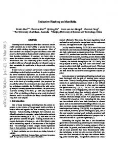
Fig. 1. The proposed method on extending p-stable distribution theory to data-dependent hashing.
of data-dependent method is the supervised hashing which not only considers data distribution, but also incorporates prior information such as class labels for supervised learning. The disadvantages of data-dependent methods is that their performance may be too dependent on the training set and they usually have limited amount of hash functions. We can see that both data-independent and data-dependent solutions have their pros and cons. An intuitive idea to overcome their shortcomings is developing an integrated strategy which combines both data-dependent hashing and dataindependent hashing, and makes them complementary to each other. To achieve this goal, we propose a hashing method based on p-stable distribution. The p-stable distribution [12] is traditionally used in data-independent hashing methods [6]. It has special mathematical properties that guarantee the distance under lp norm to be recovered by the projections on specific random vectors. In our work, we extend the p-stable distribution to the data-dependent setting. An overview of the proposed method is illustrated in Figure 1. Firstly, we project one original feature vector through multiple random vectors, and learn a single projection vector for approximating the multiple random vectors according to the data distribution. The same procedure is repeated for r times, and gives r projection vectors. This is different from LSH, which directly uses a single random vector as each projection vector, and we thus refer to our method as multiple locality sensitive hashing (MLSH). Based on MLSH, we then apply an orthogonal transformation [13] to the obtained projection vectors for preserving the Euclidean distance with binary codes. Conveniently, we refer to this process as MLSH-ITQ (MLSH with iterative quantization). Furthermore, we use the projection result of MLSH to assign quasi hash bits for some training samples and perform a label propagation [14] like process with respect to the semantic similarity to generate hash bits for the rest. We refer to this supervised hashing method as MLSH-SLP (MLSH with supervised label propagation). In [15], we introduced the p-stable distribution theory into the data-dependent hashing. This method consists of two stages. In the first stage, Gaussian random vector is directly
used to assign initial binary labels for a part of data. In the second stage, the labels of the rest data are induced according to the unsupervised similarity. In this paper, the proposed MLSH method follows a similar two-stage framework, but with completely different strategies in both stages. In the first stage, it uses the refined projection vector based on deeper analysis of the p-stable property. In the second stage, MLSH incorporates different ways based on two different scenarios. For unsupervised scenario, iterative quantization is incorporated to refine the hash functions for retrieving Euclidean neighbors. For supervised scenario, the supervised label propagation procedure is used to learn the hash functions for retrieving semantically similar instances. The contributions of this paper are summarized as follows. Firstly, based on p-stable distribution theory, we show how to view the Euclidean distance preserving problem as estimating the variance of a p-stable distribution. This observation leads to a novel projection method which maps the samples in the original feature space to arbitrary dimensional real-valued vectors. For each dimension, rather than directly using one single random vector, we generate its projection vector based on approximating the multiple random vectors for recovering the Euclidean distance within the dataset. Secondly, based on this mapping, we show how the iterative quantization method [13] can be used for minimizing the loss of thresholding. This leads to the development of the unsupervised hashing MLSH-ITQ. Finally, we construct an objective function which is similar to [7] but characterizes semantic similarity, and compute its approximate solution by combining the proposed projection method with a coordinate descent algorithm. This results in a novel supervised hashing scheme for the purpose of preserving the semantic similarity, which to a certain extent eliminates the inconsistency of feature similarity and semantic similarity in hashing. In the rest of the paper, a review of relevant hashing methods is given in Section II. The proposed unsupervised hashing is described in Section III, followed by the introduction of a novel supervised hashing in Section IV. We present the experimental results in Section V, then draw conclusions and
3
discuss the future work in Section VI. II. R ELATED W ORK Compared against its data dependent counterpart, dataindependent methods are usually considered to be more adaptive to heterogeneous data distributions, but with the decrease of efficiency in practice [7]. Locality sensitive hashing based on p-stable distribution (LSH) [6] is one of the most representative methods in the data independent hashing category. Based on the p-stable distribution, hash functions can be generated directly without any training data, and the mathematical properties of p-stable distribution [16] guarantee that vectors close to each other in the original feature space have high probability to generate the same output by each hash function. Each hash function is a random linear projection and is independent to each other because of the randomness of the projection vectors. Some other data-independent hashing schemes have been proposed besides LSH. For example, in [17], a dataindependent hashing scheme has been reported, which utilizes random Fourier features to make the Hamming distance be related to the shift-invariant kernel (e.g., Gaussian kernel) between the vectors. Recently, a kernelized locality sensitive hashing (KLSH) [11] has been proposed. It constructs random project vectors by using a weighted sum of data instances in a training set to approximate the Gaussian random hyperplane in a highly implicit kernel space. In many applications, the data distribution is not very complex and can be well learned from a training set. In this scenario, data-dependent approaches become very appealing. A representative data-dependent hashing scheme is spectral hashing (SH) [7]. It transforms the problem of finding similarity preserving code for a given dataset to a NPhard graph partitioning problem that is similar to Laplacian eigenmaps [18]. SH relaxes this problem and solve it by a spectral method [7], [18]. For novel data point, SH uses the Laplace-Beltrami eigenfunctions to obtain binary codes under the hypothesis that the data is uniformly distributed. To address the problem when data do not meet this hypothesis, anchor graph hashing (AGH) [9] has been proposed. AGH uses an anchor graph to obtain a low-rank adjacency matrix which is computationally feasible to approximate the similarity matrix and then processes it in constant time based on the Nystr¨om method [19]. Zhang et al. proposed a self-taught hashing [20] method that firstly performs Laplacian eigenmaps and then thresholds eigen-vectors to get binary code for the training set. After that, it trains an SVM classifier as the hash function for each bit. Recently, more extensions of the above methods have been developed. For instance, multidimensional spectral hashing [21] is guaranteed to maintain the affinities when the number of bits increases. Li et al. extended the spectral hashing with semantically consistent graph in [22], which incorporates prior information into SH in a supervised manner. Furthermore, Shen et al. [23] have developed a group of hashing techniques based on a wide variety of manifold learning approaches such as Laplacian eigenmaps. Dimensionality reduction methods have been widely applied into hashing problems. Several data-dependent hashing
methods have been developed based on Principal Component Analysis (PCA) [24], including PCA-Direct [13] which directly thresholds the results after performing PCA, PCARR [25] which applies a random orthogonal transformation before thresholding, PCA-ITQ [13] which refines an orthogonal transformation to reduce quantization error, and Isotropic Hashing [26] which learns orthogonal transformation that makes projected dimensions have equal variance. In [13], Gong et al. also presented a supervised hashing method CCAITQ based on Canonical Correlation Analysis (CCA) and the same iterative quantization method. LDAHash [27] introduces Linear Discriminant Analysis (LDA) [28] into hashing for local descriptors matching. Binary Reconstructive Embedding (BRE) [8] and Minimal Loss Hashing (MLH) [10] optimize objective functions directly with respect to the binary code. BRE aims to reconstruct the Euclidean distance in the Hamming space, and MLH has a hinge-like loss function. Various learning settings have been explored in data dependent hashing. Semi-supervised hashing (SSH) [29] has been introduced to search semantic similar instances when only part of the data are labelled. It minimizes the empirical error over the labeled data, and applies an information theoretic regularizer over both labeled and unlabeled data. Projection learning hashing method [30] has been proposed in a similar form as SSH, containing a semi-supervised method and an unsupervised method. Beside SSH, weaklysupervised hashing [31] and kernel-based supervised hashing (KSH) [32] are two other supervised hashing schemes that have kernel based hash functions. Kulis et al. have extended LSH functions to a learned metric [33], which can also be considered as a supervised method. Beside these methods, several other hashing methods have been proposed to address different aspects of the modelling and computation, including semantic hashing [34], random maximum margin hashing [35], Manhattan hashing [36], dual-bit quantization hashing [37], spherical hashing [38] and k-means hashing [39]. III. U NSUPERVISED H ASHING FOR P RESERVING E UCLIDEAN D ISTANCE In this section, we present our unsupervised hashing scheme MLSH-ITQ based on p-stable distribution. As illustrated in Figure 1, there are two major parts within our scheme, with one being data-independent and the other being datadependent. The core idea is to use multiple random vectors to generate one hash function. A. Euclidean Distance Preserving as Variance Estimation We commence by reviewing basics of p-stable distribution, and then describe how it can be used to preserve the original distance between data points. This process can be thought of as estimating the variance of a specific distribution. A random variable has a stable distribution if a linear combination of independent copies of the variable follows a similar distribution. For a p-stable distribution D, given t real numbers b1 ...bt and random variables X1 ...Xt which are independently and identically drawn from P distribution D, P p 1/p X, i |bi | ) i bi Xi will follow the same distribution as (
4
where X is a random variable with distribution D and p is a parameter subject to p ≥ 0 [16]. It has been proved that stable distribution exists when p ∈ (0, 2] [12]. Particularly, when p = 1 and p = 2, the corresponding p-stable distributions are Cauchy distribution and Gaussian distribution, respectively. Let w denote a d-dimensional random vector whose entries are generated independently from a standard Gaussian distribution Ds (with zero mean and unit standard deviation). Let vi and vj be two data vectors with dimensionality d, and the distribution of wT vi − wT vj = wT (vi − vj ) follows a Gaussian distribution Dg which has zero mean and variance kvi − vj k2 . Let W denote a d × r matrix whose each column is a random vector which can be thought of a vector behaving like w. The r entries of the vector W T (vi −vj ) are independent of each other and follow Dg . This implies that for arbitrary W T (vi −vj ), 1r kW T (vi −vj )k2 is an estimator of the variance of Dg . We can get the expectation of the random variable 1 T 2 r kW (vi − vj )k : 1 E[ kW T (vi − vj )k2 ] = kvi − vj k2 (1) r where k·k is the l2 norm. Equation (1) also shows that this is an unbiased estimate. Furthermore, using the probability density function of Gaussian distribution, we can get the variance of this estimator: 1 2 Var[ kW T (vi − vj )k2 ] = kvi − vj k4 (2) r r We observe that larger r leads to smaller variance and gives more precise estimation. In LSH, r corresponds to the length of hash code. Therefore, equation (2) also explains why LSH performs better with longer hash codes. B. Learning Projection Vectors The LSH scheme uses one random vector to generate one hash function (hash bit). Precise characterization of LSH requires a large number of random vector samples, which leads to long hash code. However, long hash code is less preferred in practice because it leads to low recall, sparse hash table and decreased efficiency. An intrinsic solution to overcome this disadvantage is to change the one-to-one correspondence between random vectors and hash bits. Different from LSH, we propose multiple locality sensitive hashing (MLSH) which uses c different Gaussian random vectors to generate one bit. By using c × r random vectors, our MLSH generates r hash bits. In contrast, by using the same number of random vectors, LSH results in longer code with c × r hash bits, which is less efficient. For a hashing scheme with r hash bits, our method can be implemented through estimating the variance of the Gaussian distribution Dg based on c × r random samples, which is motivated by the principles described in Section III-A. Let Q be a d × c matrix whose each column is a Gaussian random vector. If our hash function is constrained to be in a linear form, then for each hash function, our objective is finding a d-dimensional projection vector u: arg min u
n X i,j
(kQT vi − QT vj k2 − (uT vi − uT vj )2 )2
(3)
By discarding the magnitude factor, we can assume that u = Ql where l is a c-dimension unit vector, i.e., klk2 = 1. So the term kQT vi − QT vj k2 − (lT QT vi − lT QT vj )2 is always non-negative, and our objective becomes: min l
n X
(kQT vi − QT vj k2 − (lT QT vi − lT QT vj )2 )
(4)
i,j
Proposition 1. Finding the optimal solution in problem (4) is equivalent to the maximization problem: max lT QT V V T Ql l
subject to klk2 = 1.
(5)
where V is a matrix with the ith column being vi . Proof. The minimization problem in (4) can be transformed to the maximization problem as follows: arg max l
n X
(lT QT vi − lT QT vj )2
(6)
i,j
The sum of the squared pairwise difference has a proportional relation with the variance. Suppose V is a matrix with the ith column being vi , and we have: n X
(lT QT vi − lT QT vj )2 ∝ Var(lT QT V )
(7)
i,j
where Var(·) is the sample variance of elements in the vector. For the zero-mean data, Var(lT QT V ) = n1 lT QT V V T Ql. Finally, we transform the initial objective (4) in terms of the optimization problem (5). The optimal l is obtained by the eigen-decomposition of the matrix QT V V T Q, where l is the eigenvector associated with the largest eigenvalue of QT V V T Q. According to Proposition 1, this is also the optimal solution of objective (4). Therefore, the approximate solution of u for equation (3) is obtained by u = Ql. A d × r matrix ˆ is then established, with its columns being vectors resulted U from equation (5) by using r different random matrices Q 1 ˆ , and kU T (vi − vj )k2 is an separately. We have U = √c×r U 2 approximation for the estimator with variance c×r kvi − vj k4 according to equation (2). C. Minimizing the Error of Thresholding For the d × r matrix U obtained in Section III-B, let Uk denote its kth column. The binary code for a feature vector vi can be obtained by applying sign function to UkT vi . However, directly using sign(·) leads to considerable loss of accuracy in the binary code. The quantization error of thresholding can be estimated as: n X r X (sign(UkT vi ) − UkT vi )2 (8) i
k
The desired U should have a small quantization error. Note that in [6], Datar et al. quantized the real-valued output to discrete integers to maintain accuracy. Nonetheless, binary codes are more convenient for retrieval, which therefore, is adopted in this paper.
5
Algorithm 1: MLSH-ITQ Data: A d × n matrix V with each column being a feature vector in the training set; The length of hashing codes r. Result: A d × r projection matrix U . for m = 1 to r do Generate d × c matrix Q with each column being a Gaussian random vector; Perform eigen-decomposition of the matrix QT V V T Q and let l equals the eigenvector associated with the largest eigenvalue; u ← Ql; Um ← u; end 1 U ← √c×r [U1 , U2 ...Ur ]; Solve r × r orthogonal matrix R in (10) by the iterative Procrustes method in [13]; U ← U R.
Proposition 2. Given a projection matrix U and an arbitrary orthogonal r × r matrix R, U and U R have the same power for reconstructing the Euclidean distance. Proof. For an arbitrary pair of feature vectors vi and vj , we have: k(U R)T vi − (U R)T vj k2 = k(U R)T (vi − vj )k2 = (vi − vj )T (U R)(U R)T (vi − vj ) = (vi − vj )T U U T (vi − vj ) = kU T vi − U T vj k2
(9)
So the pairwise Euclidean distance of projection results under U and U R is the same. According to Proposition 2, U R behaves the same as U . In the light of this observation, we aim to obtain an optimal solution R∗ to achieve the least quantization loss of thresholding: R∗ = arg min ksign((U R)T V ) − (U R)T V k2F R
(10)
where k · kF denotes the Frobenius norm. We follow the iterative method described in [13] to solve objective function (10). In each iteration, it uses the classic Orthogonal Procrustes problem solution [40] to find an orthogonal rotation R(i) (r × r orthogonal matrix) to align vector set U T V with sign(U T V ). After updating U by U R(i) , it starts a new iteration. After t iterations, the final r × r orthogonal matrix R∗ = R(1) R(2) R(3) ...R(t) is obtained. The proposed method is summarized in Algorithm 1. D. Constructing Multiple Hash Tables For most data-dependent hashing methods, the limitation on the amount of hash functions leads to the incapability of constructing multiple hash tables. Since the matrix Q is random, our method can construct multiple hash tables in
the same way as LSH. In this setting, the Hamming distance between binary codes of vi and vj is: dist(vi , vj ) = min dHamming (Yt (vi ), Yt (vj )) t=1..L
(11)
where Yt (vi ) is the binary code of vi in the t-th hash table. In [41], [42], methods are presented to build hash tables with data-dependent strategy. However, these methods concentrate on the hash tables construction process. The idea is to train the hash functions of a data-dependent method with different data or parameters, which leads to the generation of different hash tables. Our method, on the other hand, focuses on the hashing method itself and generates multiple hash tables by random vectors subject to p-stable distribution. IV. S UPERVISED H ASHING BY I NCORPORATING S EMANTIC S IMILARITY The method presented in Section III reconstructs the Euclidean distance in the original space and learns the hash function in an unsupervised manner. In many situations, the Euclidean distance between feature vectors vi and vj does not reflect the real semantic similarity of objects. In this section, we present a supervised hashing method MLSH-SLP which explores supervised pairwise similarity. The whole procedure of this method and the relation with MLSH is shown in Figure 1. A. Hashing Objective for Semantic Similarity Let L(i) denote the class label of the object vi and S denote a matrix whose (i,j)th entry Sij represents the supervised semantic similarity between two objects i and j. Sij is defined as: ( 1, L(i) = L(j); Sij = (12) 0, otherwise. Our goal is to learn binary codes subject to the requirement that neighboring samples in the same class are mapped to similar codes in the Hamming space. The neighborhood of object samples is measured in terms of semantic similarity. In this scenario, our method seeks an r-bit Hamming embedding1 Y ∈ {0, 1}r×n for n samples in the original space, and learns r hash functions h1,2,...,r : Rd → {0, 1}. Let yi denote the ith column of Y , i.e., the binary code for object vi . We have an intuitive objective: X Sij kyi − yj k2 (13) arg min Y
i,j
subject to: yi ∈ {0, 1}r×1,
n X i
yi =
n 1r 2
where every column of Y should be independent of each other. Pn 1r isn an r-dimensional vector of ones. The constraint i yi = 2 1r enables the data to be mapped into the hash table uniformly. Minimizing (13) leads to small Sij being associated with large Hamming distance kyi − yj k2 , and viceversa. 1 Though slightly different, this definition is equivalent to the previous binary output {-1,1}.
6
p(m)
i,j
(m)
subject to pi
∈ [0, 1]
The method for obtaining optimal p(m) satisfying (14) is described in the following two subsections. B. Quasi Hash Bits In this subsection, we present a strategy for initializing the (m) hash probability pi , i.e., the probability for the mth hash function to map the feature vector vi to 1. We commence by generating a d-dimensional vector u by using the MLSH presented in Section III. Then, for samples i = 1, ..., n in the (m) training set, pi is initialized as follows: uT vi > α+ ; 1, (m) (15) pi = 0, uT vi < α− ; 0.5, otherwise.
Here α+ and α− , which represent positive and negative threshold parameters respectively, will be set empirically. The initialization strategy is developed in the light of the intuition that if the Euclidean distance between feature vectors of two objects is very large, then it is nearly impossible that they are semantic neighbors. Note that we have already shown that the difference of projections on u could reflect the Euclidean distance between the original vectors. If kpi − pj k2 > 0, which means sign(uT vi ) 6= sign(uT vj ), then |uT vi − uT vj | > α+ − α− . Suppose α+ − α− is large enough, Sij = 0 will be with a high probability. When kpi − pj k2 = 0, Sij will not T influence the sum. Furthermore, P (m) u vi has a zero mean which approximately satisfies i yi = n/2, and the randomness of u makes y (m) (m = 1, 2...r) independent of each other. Therefore, this partial solution satisfies the constraints in equation (13). (m) For the time being, we set the hash bit yi for vi to be 1 (m) (m) if pi = 1, and set it to be 0 if pi = 0. We refer to these
hash bits thus obtained as quasi hash bit. Furthermore, the remaining feature vectors associated with the hash probability 0.5 tend to be less distinctive in terms of the projection on u, and we do not assign quasi hash bits to them. C. Coordinate Descent In this subsection, we use the coordinate descent method to iteratively update the hash probabilities which are not associated with quasi hash bits. In each iteration, we minimize the objective function (14) by setting the derivative with (m) (m) to be zero. Specifically, we treat one pi respect to pi with the initial value 0.5 as a unique variable, hold all the (m) other hash probabilities fixed, and update pi as follows: (m)
pi
=
n X
j=1,j6=i
(m)
Sij pj Pn
k=1,k6=i
Sik
.
(16)
Suppose we have in total n′ hash probabilities which are not associated with quasi hash bits. The coordinate descent method behaves in a way that one loop of iterations enumerate all the n′ hash probabilities and then starts another loop of iterations. (m) (m) Since Sij is always non-negative, and kpi − pj k2 is convex, problem (14) is a convex optimization problem which means it has global optimal solution. Furthermore, the subproblem of the coordinate descent method is also convex, P (m) (m) so the objective value i,j Sij kpi − pj k2 decreases after each iteration. Figure 2 shows the convergence process of the optimization method for solving the problem (14) on the CIFAR-10 dataset. Details on this dataset are presented in Section V. 4
5
x 10
4.98 4.96 4.94 Objective value
Weiss et al. [7] have shown that a similar problem to Equation (13) is NP hard. Their solution is relaxation of the problem to that of eigen-decomposition, which is based on the similarity measured in the original feature space. In contrast, we exploit semantic similarity and approximate a solution using the p-stable distribution theory and a coordinate descent method. Let y (m) be an n-dimensional row vector denoting the mth row of Y . We transform the original problem of learning Y ∈ {0, 1}r×n to r subproblems of learning y (m) ∈ {0, 1}1×n(m = 1, 2...r). Then each row vector y (m) could be learned separately for m = 1, 2, ..., r through the same (m) learning strategy. Let yi denote the ith element in y (m) , we relax the original problem with a probabilistic form. Let p(m) (m) be an n-dimensional vector with the ith component pi being (m) the probability for yi = 1, i.e., the probability of vi having the binary output 1 with respect to the mth hash function. The (m) (m) (m) (m) (m) expectation of yi is E[yi ] = pi ·1+(1−pi )·0 = pi . We formulate the objective function for the mth subproblem of all the r subproblems as follows: X (m) (m) (14) Sij kpi − pj k2 arg min
4.92 4.9 4.88 4.86 4.84 4.82
1
3
5 # Outer loops
7
9
Fig. 2. Numerical result of the convergency of the optimization process on the CIFAR-10 dataset.
After p(m) converges, we get the refined hash probabilities. Then for one sample vi which is not assigned a quasi hash bit, we generate its binary code with respect to the mth hash function as follows: ( (m) 1, pi > 0.5; (m) yi = (17) 0, otherwise. Repeat this procedure r times, r n-dimensional row vectors can be generated. Finally, the {0, 1}r×n matrix Y can be established by concatenating the r n-dimensional row vectors.
7
D. Binary Codes for Queries The scheme presented in Section IV-C only generates the binary representations for samples in the training set. In this subsection, we investigate how to generate the codes of a query. According to the definition of hashing, one hash function hm maps a sample vi in the original feature space (m) ∈ {0, 1}. In this scenario, one hash to a binary value yi function can be considered as a binary classifier. Therefore, generating the binary code for a query can be thought of as a binary classification problem. We use the training dataset consisting of vi for i = 1, · · · , n and the corresponding r-bit Hamming embedding Y obtained in Section IV-C to train r binary classifiers. The mth binary classifier categorizes a query into the class with label 0 or 1, which is the mth binary code for the query accordingly. Therefore, it is reasonable to refer to the mth binary classifier as the mth hash function hm . E. A Label Propagation View of the Proposed Framework We consider one hash function as a binary classifier and the hash bits as the labels of samples. For normal classification problems, the labels of training samples are usually obtained through human annotation. On the other hand, for a hash function, a sample is assigned a hash bit. Specifically, the criterion for this assignment is based on equation (13), which is intrinsically similar to that of label propagation. Different from general label propagation that uses feature similarity to propagate the label, our method uses semantic similarity to propagate the hash bits. However, our method and label propagation share the common underlying principle that one classifier should assign the same class labels to neighboring samples with a high probability. Therefore, we refer to our method described in this section as multiple locality sensitive hashing with supervised label propagation (MLSH-SLP). The detail of the whole procedure is described in Algorithm 2. V. E XPERIMENTS A. Datasets and Experiments Setup We evaluated the performance of the proposed methods on three popular image datasets. These datasets vary in content, image sizes, class labels, and human annotations. CIFAR-10 dataset [43] consists of 60,000 32×32 color images in 10 classes, with 6,000 images per class. The classes include airplane, automobile, bird, cat, deer, dog, frog, horse, ship, and truck. Figure 3 shows some sample images randomly selected from each class. MNIST database consists of 70,000 handwritten digit images, including 60,000 examples in the training set, and 10,000 examples in the test set. It is a subset extracted from a larger set available from NIST. The images are 28 × 28 grey scale. This dataset has 10 classes corresponding to the 0∼9 digits, with all images being labeled. NUS-WIDE is a web image dataset created by the Lab for Media Search in National University of Singapore, which contains 269,648 images downloaded from Flickr. The groundtruth of these images are provided in multiple labels such that each image is labeled as a vector of zeros and ones to represent
Algorithm 2: MLSH-SLP Data: A d × n matrix V with each column being a feature vector in the training set; A similarity matrix S; The length of hashing codes r. Result: Binary codes Y ; A set of r hash functions hm (·) for m = 1, 2, ..., r. for m = 1 to r do Generate a vector u as described in Section III-B; (m) Initialize pi according to (15); for i = 1 to n do (m) if pi = 1 then Assign a quasi hash bit 1 to vi ; end (m) if pi = 0 then Assign a quasi hash bit 0 to vi ; end end while p(m) is not converged do for i = 1 to n do if vi does not have a quasi hash bit then (m) P Sij p (m) pi ← nj=1,j6=i Pn j Sik ; k=1,k6=i
end end end Assign y (m) according to (17); hm ←Classifier(V , y (m) ); end Y = [y (1)T , y (2)T , ..., y (r)T ]T .
whether it belongs to one of the 81 defined concepts. Each image can be assigned with multiple concepts. We extracted different image features on each dataset due to different properties of corresponding images. For CIFAR-10, the images are too small to extract good scale invariant local features such as SIFT [44]. Considering that images are in the same size, we used a 512-dimensional GIST descriptor [3] to represent each image. In MNIST, the digit in each image is well aligned, so the gray values of each image can be treated as a 784-dimension feature vector. Since a major portion of pixels are clean background pixels, each feature vector has a sparse form. Images in NUS-WIDE are in larger size and contain lots of detail information. In the experiments, we used the 500-dimensional Bag-of-Words [2] feature vector built from SIFT descriptions for image retrieval. The proposed MLSH-SLP method can work with various classifiers. In the experiments, we chose linear SVM as the model of hash function in order to meet the efficiency requirements of image retrieval. The linear model is efficient in the prediction phase, which is very important to the indexing time. In the implementation, we employed the LIBLINEAR [45] which has low time complexity and good classification accuracy. The main parameters are set as default values provided by LIBLINEAR, i.e., cost C = 1, dual maximal violation tolerance ǫ = 0.1.
8
then the precision-recall curve is plotted. As a complement, we also calculated the mean average precision (mAP), which is the area under the precision-recall curve. In practice, there are two major applications for the resulted hash binary codes, i.e. Hamming ranking and hash lookup. Hamming ranking compares the binary code of the query with all samples in the database, which leads to linear complexity but can be efficient thanks to the efficacy of the comparison operator of binary codes. Hamming ranking is usually used with longer code length. Hash lookup constructs a lookup table for the database. With the binary code of a query, it retrieves samples that fall within a bucket of the Hamming radius δ. To guarantee the efficiency of retrieval, the lookup table should not be too sparse and the binary code should be compact. In our experiments, we also compute the mean precision under different hash code lengths for the Hamming radius δ and the top k returned samples of Hamming ranking: P Number of retrieved relevant samples for query i mean precision =
Fig. 3. Random samples from the CIFAR-10 dataset. Each row contains 10 images of one class.
B. Evaluation Protocols and Baseline Methods In the experiments, we evaluated the proposed MLSH-ITQ and MLSH-SLP methods in both unsupervised and supervised settings. In the unsupervised setting, we used the Euclidean neighbors as the ground truth. Similar to [17], we used the average distance of all query samples to the 50th nearest neighbor as a threshold to determine whether a point in the dataset should be considered as a true positive for a query. In the supervised setting, we used class labels as the ground truth. In the CIFAR-10 dataset and the MNIST dataset, each image has a single class label, then images in the same class are considered as the true neighbors to each other. While on NUS-WIDE dataset, we followed the protocol in [29] such that the ground truth is determined based on whether two samples share at least one semantic label. We randomly chose 1000 samples from each dataset as the query images, and used the rest of the dataset as the target of the search. For MLSH-ITQ, we used all samples but the query images in the dataset as the training set. We randomly selected 2000 samples from each dataset for training MLSHSLP because of its relatively high computational complexity. We used the same size of training sets as described in their original papers for all alternative methods. We adopted the precision-recall curve to compare the overall performance of all methods. In our experiments, it was computed by: precision =
Number of retrieved relevant pairs Total number of retrieved pairs
(18)
recall =
Number of retrieved relevant pairs Total number of relevant pairs
(19)
For the given queries, we increase the Hamming radius from 0 to r to generate r + 1 pairs of precision and recall values,
i
Total number of retrieved samples for query i
Number of test samples
(20) If there is nothing in the buckets (i.e., no retrieved samples) for certain Hamming radius δ and query sample, we consider it to be zero precision. We compared our methods with some state-of-the-art unsupervised hashing methods, which include iterative quantization based on PCA (PCA-ITQ) [13], k-means hashing (KMH) [39], spherical hashing (SPH) [38], unsupervised sequential learning hashing (USPLH) [30], spectral hashing (SH) [7], and locality sensitive hashing (LSH) [6]. For supervised or semi-supervised hashing methods, we evaluated iterative quantization based on CCA (CCA-ITQ) [13], semi-supervised hashing (SSH) [29] and semi-supervised sequential projection learning hashing (S3PLH) [30]. In these methods, LSH and our method MLSHITQ can directly construct multiple hash tables, we denote them as LSH-m and MLSH-ITQ-m, respectively. A summary on different properties of these methods is given in Table I. Method
Hash Function
Learning Paradigm
PCA-ITQ [13] KMH [39] SPH [38] USPLH [30] SH [7] LSH [6] CCA-ITQ [13] SSH [29] S3PLH [30]
linear nonlinear nonlinear linear nonlinear linear linear linear linear
unsupervised unsupervised unsupervised unsupervised unsupervised (data-independent) supervised semi-supervised semi-supervised
TABLE I S UMMARY OF PROPERTIES OF HASHING METHODS UNDER COMPARISON .
Through Table I, we observe that hash functions in PCAITQ, CCA-ITQ, LSH, SSH, USPLH and S3PLH have the linear form of hash functions, which are the same as our methods. On the other hand, KMH, SPH and SH use nonlinear hash functions, but still achieve a constant time complexity for computing binary codes.
9
0.8 0.25 0.6 mAP
mAP
0.2 0.15 0.1
0.4 0.2
0.05 0
0 9
9 7
7 9
5 L
3
L
5 1
3 1
9
5
7
7
3
5 1
c
3 1
(a) CIFAR-10
c
(b) MNIST
Fig. 4. The mAP of different parameter settings for MLSH-ITQ-m on CIFAR-10 and MNIST.
C. Evaluation of Unsupervised Hashing Methods Unsupervised hashing methods aim at finding the nearest neighbors of the query according to the Euclidean distance. They were originally developed for improving the time efficiency of nearest neighbor search. Because the class labels are not available, the results depend on the distribution of the data. We chose two datasets, i.e., CIFAR-10 and MNIST which have distinctive data distributions. GIST descriptors were extracted from CIFAR-10, which usually consists of nonzero real numbers. On the other hand, features extracted from MNIST are sparse vectors, with most entries being zeros. After setting the ground truth by Euclidean distance as in section V-B, we compared LSH, SH, USPLH, SPH, KMH, PCA-ITQ and the proposed method MLSH-ITQ. There are two parameters in our method, the number of random vectors for one bit c, and the number of constructed hash tables L. We set them with different values ranging from 1 to 9, and computed the mAP on each parameter setting. Figure 4 shows the mAP of different parameter settings on CIFAR-10 and MNIST. When using multiple hash tables, we returned samples within certain Hamming distance δ in all L hash tables. Therefore, the recall always goes up with the increase of L, but the precision does not. Because mAP is computed as the area under the precision-recall curve, too large L will decrease it. Large c can decrease the variance of the Euclidean distance estimator according to Section III-A, but may increase the approximation error in equation (4). Because we use the eigen-decomposition based method solve l, too large c will dilute the information of the eigenvector corresponding to the largest eigenvalue. We can see that too large or too small values for both L and c do not lead to good performance. Therefore, in the following experiments, we set L = 7 and c = 3 for both CIFAR-10 and MNIST. Figures 5 and 6 show precision-recall curves for Euclidean neighbor retrieval on CIFAR-10 and MNIST, respectively. On CIFAR-10, our method with multiple hash tables (MLSH-
ITQ-m) outperforms all alternative methods when the code length is 32. When the code length equals 64 or 128, the performances of MLSH-ITQ-m and PCA-ITQ are very close. Our method with single a hash table (MLSH-ITQ) outperforms all alternatives except PCA-ITQ, and its performance is very close to PCA-ITQ when the code length is greater than 64. For the alternative methods, LSH and SPH have significant improvement when the code length increases. USPLH, SH, and KMH do not work well on CIFAR-10. On MNIST, KMH and USPLH have better performance and SPH performs the worst. Although both LSH and our method are based on the pstable distribution, our method outperforms LSH significantly because of the data-dependent component. This superiority is more obvious with short code length because our method takes the data distribution into consideration. To take the quantitative evaluation of the hash techniques one step further, we used the mean precision and recall of Hamming radius δ to evaluate different methods for hash lookup. Similar to many other hashing methods, we set the Hamming radius δ < 2, and computed the recall according to (19) and the mean precision according to (20). Figures 7 and 8 illustrate these two measurements with respect to the length of hashing codes, respectively. When the hash code length r goes too large, the hash table becomes too sparse. For a given query, the buckets within Hamming radius δ may contain nothing, so the precision is looked as zero. Therefore, the performance with Hamming radius δ may degrade when the code length r increases. It is clear that our single hash table method MLSH-ITQ outperforms alternative single table methods. We also observe that the MLSH-ITQ benefits from using multiple hash tables for hash lookup, because MLSH-ITQ-m has demonstrated significant advantages over the alternative methods. Furthermore, we make an empirical comparison between MLSH-ITQ-m and LSH-m, under different number of hash tables. Figure 9 shows the mAP for LSH-m and MLSH-ITQ-m
10
1
1 MLSH-ITQ MLSH-ITQ−m KMH SPH PCA−ITQ USPLH SH LSH
Precision
0.7 0.6
0.8 0.7
0.5
0.6
0.8 0.7
0.5
0.6 0.5
0.4
0.4
0.3
0.3
0.3
0.2
0.2
0.2
0.1
0.1
0
0
0.2
0.4
0.6
0.8
0
1
MLSH-ITQ MLSH-ITQ−m KMH SPH PCA−ITQ USPLH SH LSH
0.9
Precision
0.8
1
MLSH-ITQ MLSH-ITQ−m KMH SPH PCA−ITQ USPLH SH LSH
0.9
Precision
0.9
0.4
0.1
0
0.2
0.4
0.6
0.8
0
1
0
0.2
0.4
Recall
Recall
(a) 32 bits
0.6
0.8
1
0.8
1
Recall
(b) 64 bits
(c) 128 bits
1
1
0.9
0.9
0.8
0.8
0.8
0.7
0.7
0.7
0.6
0.6
0.6
0.5 MLSH-ITQ MLSH-ITQ-m KMH SPH PCA−ITQ USPLH SH LSH
0.4 0.3 0.2 0.1 0
0
0.2
0.5 MLSH-ITQ MLSH-ITQ−m KMH SPH PCA−ITQ USPLH SH LSH
0.4 0.3 0.2 0.1 0.4
0.6
0.8
0
1
Precision
1 0.9
Precision
Precision
Fig. 5. Precision-recall curves on CIFAR-10, using Euclidean ground truth.
0
0.2
MLSH-ITQ MLSH-ITQ−m KMH SPH PCA−ITQ USPLH SH LSH
0.4 0.3 0.2 0.1 0.4
Recall
0.5
0.6
0.8
1
0
0
0.2
0.4
Recall
(a) 32 bits
0.6 Recall
(b) 64 bits
(c) 128 bits
Fig. 6. Precision-recall curves on MNIST, using Euclidean ground truth.
0.2
0.5
0.18 0.16
Mean precision
0.14 0.12 0.1 0.08 0.06
0.4 0.35 0.3 0.25 0.2 0.15
0.04
0.1
0.02
0.05
0
MLSH-ITQ MLSH-ITQ−m KMH SPH PCA−ITQ USPLH SH LSH
0.45
Mean precision
MLSH-ITQ MLSH-ITQ−m KMH SPH PCA−ITQ USPLH SH LSH
16
32
48 Length of hashing codes
64
80
0
16
(a) CIFAR-10 Fig. 7. Mean precision in Hamming radius δ < 2 on CIFAR-10 and MNIST, using Euclidean ground truth.
32
48 Length of hashing codes
(b) MNIST
64
80
11
1
0.45 MLSH-ITQ MLSH-ITQ−m KMH SPH PCA−ITQ USPLH SH LSH
0.4 0.35
0.25
0.8 0.7 0.6 Recall
Recall
0.3
0.2
MLSH-ITQ MLSH-ITQ−m KMH SPH PCA−ITQ USPLH SH LSH
0.9
0.5 0.4
0.15
0.3
0.1
0.2
0.05
0.1
0
16
32
48 Length of hashing codes
64
0
80
16
32
(a) CIFAR-10
48 Length of hashing codes
64
80
(b) MNIST
Fig. 8. Recall in Hamming radius δ < 2 on CIFAR-10 and MNIST, using Euclidean ground truth.
0.24
0.75
0.22
0.7
0.2
0.65 mAP
0.8
mAP
0.26
0.18
0.6
0.16
0.55
0.14
0.12
MLSH-ITQ−m LSH−m 1
3
5 7 Number of hash tables L
9
11
(a) CIFAR-10
0.5
0.45
MLSH-ITQ−m LSH−m 1
3
5 7 Number of hash tables L
9
11
(b) MNIST
Fig. 9. The mAP for LSH-m and MLSH-ITQ-m with code length 48.
with the fixed code length r = 48. It is clear that our proposed method outperforms LSH-m. And in most cases, both methods have better performance with more hash tables, and the mAP of MLSH-ITQ-m changes slightly when L ≥ 5. It is also clear from the experimental results that the dataindependent methods perform better with longer code length. The reason for this is that the data-independent methods rely on random projections. The larger number of projections they have, the more precise they can recover the original distance. On the other hand, data-dependent methods capture the distribution of data, so they usually have good performance with relatively short code length. D. Evaluation of Supervised Hashing Methods In some practical applications, the neighborhood of a given query is not based on simple metric such as Euclidean distance, but relies on the semantic similarity such as whether two samples belong to the same class. Therefore, we used the class labels of image samples as the ground truth. We compared the proposed MLSH-SLP method with several alternative hashing
methods including LSH [6], SH [7], S3PLH [30], SSH [29], and CCA-ITQ [13]. Figure 10 shows the mean average precision under different code lengths on each dataset. The proposed MLSH-SLP method achieves the best results on all three datasets, and performs better with longer code. S3PLH gets the secondbest rank on both CIFAR-10 and MNIST. LSH performs the second-best on NUS-WIDE. For the other methods under comparison, SH and SSH generate poor mAP, though SSH sometimes performs better than SH on NUS-WIDE. The mAP of CCA-ITQ degrades when the code length increases. The reason may be that CCA-ITQ is based on the Canonical Correlation Analysis which usually has good performance with low dimensional output. If the dimensionality of the output becomes higher, the useless dimensions of output may be introduced and will tarnish the useful dimensions. It should be noted that some methods do not generate consistent performance on different dataset. On CIFAR-10 and MNIST datasets, LSH has lower mean average precision than S3PLH, but on NUS-WIDE, LSH exceeds S3PLH. We can find that
12
0.26
0.8
0.24
0.7
0.23
0.22
0.22 0.6 0.21 0.2
MLSH-SLP CCA−ITQ SSH S3PLH SH LSH
0.18
mAP
mAP
mAP
0.5 0.2
0.4 0.16 0.19 0.3 0.14 0.18
0.2
0.12 0.1
32
64
128 Length of hashing codes
0.1
256
32
64
(a) CIFAR-10
128 Length of hashing codes
0.17
256
32
64
(b) MNIST
128 Length of hashing codes
256
(c) NUS-WIDE
Fig. 10. The mAP on CIFAR-10, MNIST, and NUS-WIDE, using class label ground truth.
0.4
0.35
0.85
0.26
0.8
0.25
0.75
0.24
0.3
0.25
0.23 Mean precision
Mean precision
Mean precision
0.7 0.65 0.6 0.55
0.19
0.45
0.18
0.4
32
48
64 80 96 Length of hashing codes
(a) CIFAR-10
112
128
0.35
0.21 0.2
0.5 0.2
MLSH-SLP CCA−ITQ SSH S3PLH SH LSH
0.22
32
48
64 80 96 Length of hashing codes
(b) MNIST
112
128
0.17
32
48
64 80 96 Length of hashing codes
112
128
(c) NUS-WIDE
Fig. 11. Mean precision of top 500 Hamming neighbors on CIFAR-10, MNIST, and NUS-WIDE, using class label ground truth.
LSH performs better than many supervised methods on NUSWIDE. This is because the Bag-Of-Words features used in NUS-WIDE can represent the content well, i.e., the Euclidean distance between the features can already give a good retrieval result. We also show in Figure 11 the mean precision of top 500 Hamming neighbors. The code length r is in range [32, 128]. It is clear that MLSH-SLP outperform the alternatives methods with a large margin on all datasets. S3PLH performs well on CIFAR-10, but has a low precision on NUS-WIDE. The mean precision of CCA-ITQ is lower with longer code. In general, CCA-ITQ and SSH perform better with compact hash code than other methods which do not use the supervised information. Finally, we show samples of retrieved images on the CIFAR10 dataset in Figure 12 with false positives labeled by red rectangles. This figure gives a qualitative evaluation of the retrieval performance of different methods. E. Computational Cost Table II shows the training and indexing time on CIFAR-10 from each method. All experiments were implemented using MATLAB, and ran on a PC with Core-i7 3.4GHZ CPU and 16GB memory. LSH does not have a training phase because it is a data-independent method. We find that MLSH-SLP, KMH and USPLH take the highest training time. In the training procedure of MLSH-SLP, doing propagation and training the SVM classifier cost the majority of time. Although the training phase of MLSH-SLP is time consuming, it can be boosted
with parallel computing because training each hash function is independent. Almost all methods require only short indexing time expect SH which has a more complex nonlinear hash function that takes a longer time to get the binary code. When multiple hash tables are used, the training time and indexing time will be L times longer than the single hash table version. This can also be reduced if we generate the hash functions and binary codes in parallel. VI. C ONCLUSION In this paper, we have reviewed the properties of p-stable distribution and shown how to incorporate it with training data in data dependent setting. We have presented MLSHITQ which takes the distribution of data into consideration. It combines multiple random projections for minimizing the differences between pairwise distances of binary codes and original vectors. Repeating the same procedure r times, we can generate a vector in Rr . We have also used an orthogonal transformation to minimize the thresholding error, making binary codes accurately preserve the Euclidean distance. Compared with data-independent hashing such as LSH, this method improves the performance under compact binary codes. In practice, we can build multiple hash tables to improve the precision and recall rate while most data-dependent hashing can only use a single hash table. For ANN search based on semantic similarity, we extend our method with supervised information. We have proposed a supervised hashing method (MLSH-SLP), whose training procedure is similar to label propagation. For each bit, we use the p-stable properties to
13
MLSH-SLP
CCA-ITQ
SSH
S3PLH
SH
LSH
query
Fig. 12. Qualitative results on CIFAR-10. We retrieved 25 Hamming neighbors of some query examples under 48-bit hashing codes using each methods, and show the false positives in red rectangle. Methods MLSH-SLP MLSH-ITQ S3PLH USPLH SSH LSH SH SPH KMH PCA-ITQ CCA-ITQ
32 bits Training Time Indexing Time 58.19 0.19 2.81 0.04 18.62 0.08 55.11 0.08 1.09 0.08 0.11 0.71 0.51 7.44 0.19 117.02 1.22 2.55 0.12 3.03 0.13
64 bits Training Time Indexing Time 115.87 0.24 5.8 0.08 36.62 0.14 111.73 0.14 1.1 0.15 0.16 0.89 1.84 14.33 0.24 128.44 1.26 4.87 0.23 4.96 0.21
128 bits Training Time Indexing Time 230.78 0.39 12.66 0.18 73.75 0.26 225.56 0.25 1.22 0.26 0.29 1.17 6.97 27.56 0.38 156.88 1.35 10.69 0.39 10.71 0.39
256 bits Training Time Indexing Time 463.13 0.63 31.59 0.41 147.57 0.46 448.98 0.5 1.9 0.52 0.53 1.87 27.2 61.41 0.67 215.37 1.57 27.91 0.84 27.14 0.82
TABLE II T RAINING AND INDEXING TIME ( SECONDS ) ON CIFAR-10.
assign the quasi bits to a portion of samples in the training set, and then optimize the assignment of hash bits to the remaining samples according to the semantic similarity. We have evaluated these two hashing methods on three public image data sets. Compared with several state-of-the-art hashing approaches, the proposed methods have shown their superiority. MLSH-ITQ with multiple hash tables has achieved the best results for unsupervised cases and MLSH-SLP has produced the best performance for the supervised setting. In the future, we will expand this idea to other problems such as clustering or dimensionality reduction. R EFERENCES [1] J. L. Bentley, “Multidimensional binary search trees used for associative searching,” Communications of the ACM, vol. 18, no. 9, pp. 509–517, 1975. [2] S. Lazebnik, C. Schmid, and J. Ponce, “Beyond bags of features: spatial pyramid matching for recognizing natural scene categories,” in Proceedings of the IEEE Conference on Computer Vision and Pattern Recognition, vol. 2, 2006, pp. 2169–2178.
[3] A. Oliva and A. Torralba, “Modeling the shape of the scene: A holistic representation of the spatial envelope,” International Journal of Computer Vision, vol. 42, no. 3, pp. 145–175, 2001. [4] R. Weber, H.-J. Schek, and S. Blott, “A quantitative analysis and performance study for similarity-search methods in high-dimensional spaces,” in Proceedings of the International Conference on Very Large Data Bases, 1998, pp. 194–205. [5] P. Indyk and R. Motwani, “Approximate nearest neighbors: towards removing the curse of dimensionality,” in Proceedings of the Annual ACM symposium on Theory of computing, 1998, pp. 604–613. [6] M. Datar, N. Immorlica, P. Indyk, and V. Mirrokni, “Locality-sensitive hashing scheme based on p-stable distributions,” in Proceedings of the Annual Symposium on Computational Geometry, 2004, pp. 253–262. [7] Y. Weiss, A. Torralba, and R. Fergus, “Spectral hashing,” in Proceedings of the Neural Information Processing Systems Conference, 2008, pp. 1753–1760. [8] B. Kulis and T. Darrell, “Learning to hash with binary reconstructive embeddings,” Proceedings of the Neural Information Processing Systems Conference, vol. 22, pp. 1042–1050, 2009. [9] W. Liu, J. Wang, S. Kumar, and S.-F. Chang, “Hashing with graphs,” in Proceedings of the International Conference on Machine Learning, 2011, pp. 1–8. [10] M. Norouzi and D. J. Fleet, “Minimal loss hashing for compact binary codes,” in Proceedings of the International Conference on Machine Learning, 2011, pp. 353–360. [11] B. Kulis and K. Grauman, “Kernelized locality-sensitive hashing,” IEEE
14
[12] [13]
[14] [15] [16] [17] [18] [19] [20]
[21] [22] [23] [24] [25]
[26] [27]
[28] [29] [30] [31] [32] [33] [34] [35] [36]
Transactions on Pattern Analysis and Machine Intelligence, vol. 34, no. 6, pp. 1092–1104, 2012. V. Zolotarev, One-dimensional stable distributions. American Mathematical Society, 1986, vol. 65. Y. Gong, S. Lazebnik, A. Gordo, and F. Perronnin, “Iterative quantization: A procrustean approach to learning binary codes for large-scale image retrieval,” IEEE Transactions on Pattern Analysis and Machine Intelligence, vol. 35, no. 12, pp. 2916–2929, 2013. X. Zhu and Z. Ghahramani, “Learning from labeled and unlabeled data with label propagation,” Technical Report CMU-CALD-02-107, Carnegie Mellon University, Tech. Rep., 2002. H. Yang, X. Bai, C. Liu, and J. Zhou, “Label propagation hashing based on p-stable distribution and coordinate descent,” in Proceedings of the International Conference on Image Processing, 2013. P. Indyk, “Stable distributions, pseudorandom generators, embeddings and data stream computation,” in Proceedings of the Annual Symposium on Foundations of Computer Science, 2000, pp. 189–197. M. Raginsky and S. Lazebnik, “Locality-sensitive binary codes from shift-invariant kernels,” Proceedings of the Neural Information Processing Systems Conference, vol. 22, pp. 1509–1517, 2009. M. Belkin and P. Niyogi, “Laplacian eigenmaps and spectral techniques for embedding and clustering,” Proceedings of the Neural Information Processing Systems Conference, vol. 14, pp. 585–591, 2001. Y. Bengio, O. Delalleau, N. L. Roux, J.-F. Paiement, P. Vincent, and M. Ouimet, “Learning eigenfunctions links spectral embedding and kernel pca,” Neural Computation, vol. 16, no. 10, pp. 2197–2219, 2004. D. Zhang, J. Wang, D. Cai, and J. Lu, “Self-taught hashing for fast similarity search,” in Proceedings of the International ACM SIGIR Conference on Research and Development in Information Retrieval, 2010, pp. 18–25. Y. Weiss, R. Fergus, and A. Torralba, “Multidimensional spectral hashing,” in Proceedings of the European Conference on Computer Vision, 2012, pp. 340–353. P. Li, M. Wang, J. Cheng, C. Xu, and H. Lu, “Spectral hashing with semantically consistent graph for image indexing,” IEEE Transactions on Multimedia, vol. 15, no. 1, pp. 141–152, 2013. F. Shen, C. Shen, Q. Shi, A. v. d. Hengel, and Z. Tang, “Inductive hashing on manifolds,” Proceedings of the IEEE Conference on Computer Vision and Pattern Recognition, 2013. I. T. Jolliffe, Principal Component Analysis. Springer-Verlag New York, 1986, vol. 487. H. J´egou, M. Douze, C. Schmid, and P. P´erez, “Aggregating local descriptors into a compact image representation,” in Proceedings of the IEEE Conference on Computer Vision and Pattern Recognition, 2010, pp. 3304–3311. W. Kong and W.-J. Li, “Isotropic hashing,” in Proceedings of the Neural Information Processing Systems Conference, 2012, pp. 1655–1663. C. Strecha, A. M. Bronstein, M. M. Bronstein, and P. Fua, “Ldahash: Improved matching with smaller descriptors,” IEEE Transactions on Pattern Analysis and Machine Intelligence, vol. 34, no. 1, pp. 66–78, 2012. R. A. Fisher, “The use of multiple measurements in taxonomic problems,” Annals of Eugenics, vol. 7, no. 2, pp. 179–188, 1936. J. Wang, S. Kumar, and S. Chang, “Semi-supervised hashing for large scale search,” IEEE Transactions on Pattern Analysis and Machine Intelligence, vol. 34, no. 12, pp. 2393–2406, 2012. J. Wang, S. Kumar, and S.-F. Chang, “Sequential projection learning for hashing with compact codes,” in Proceedings of the International Conference on Machine Learning, 2010, pp. 1127–1134. Y. Mu, J. Shen, and S. Yan, “Weakly-supervised hashing in kernel space,” in Proceedings of the IEEE Conference on Computer Vision and Pattern Recognition, 2010, pp. 3344–3351. W. Liu, J. Wang, R. Ji, Y. Jiang, and S. Chang, “Supervised hashing with kernels,” in Proceedings of the IEEE Conference on Computer Vision and Pattern Recognition, 2012, pp. 2074–2081. B. Kulis, P. Jain, and K. Grauman, “Fast similarity search for learned metrics,” IEEE Transactions on Pattern Analysis and Machine Intelligence, vol. 31, no. 12, pp. 2143–2157, 2009. R. Salakhutdinov and G. Hinton, “Semantic hashing,” International Journal of Approximate Reasoning, vol. 50, no. 7, pp. 969–978, 2009. A. Joly and O. Buisson, “Random maximum margin hashing,” in Proceedings of the IEEE Conference on Computer Vision and Pattern Recognition, 2011, pp. 873–880. W. Kong, W.-J. Li, and M. Guo, “Manhattan hashing for large-scale image retrieval,” in Proceedings of the International ACM SIGIR Conference on Research and Development in Information Retrieval, 2012, pp. 45–54.
[37] W. Kong and W.-J. Li, “Double-bit quantization for hashing,” in Proceedings of the AAAI Conference on Artificial Intelligence, 2012. [38] J.-P. Heo, Y. Lee, J. He, S.-F. Chang, and S.-E. Yoon, “Spherical hashing,” in Proceedings of the IEEE Conference on Computer Vision and Pattern Recognition, 2012, pp. 2957–2964. [39] K. He, F. Wen, and J. Sun, “K-means hashing: an affinity-preserving quantization method for learning binary compact codes,” in Proceedings of the IEEE Conference on Computer Vision and Pattern Recognition, 2013, pp. 2938–2945. [40] P. H. Sch¨onemann, “A generalized solution of the orthogonal procrustes problem,” Psychometrika, vol. 31, no. 1, pp. 1–10, 1966. [41] H. Xu, J. Wang, Z. Li, G. Zeng, S. Li, and N. Yu, “Complementary hashing for approximate nearest neighbor search,” in Proceedings of the International Conference on Computer Vision, 2011, pp. 1631–1638. [42] X. Liu, J. He, and B. Lang, “Reciprocal hash tables for nearest neighbor search,” in Proceedings of the AAAI Conference on Artificial Intelligence, 2013. [43] A. Krizhevsky and G. Hinton, “Learning multiple layers of features from tiny images,” Master’s thesis, Department of Computer Science, University of Toronto, 2009. [44] D. Lowe, “Distinctive image features from scale-invariant keypoints,” International Journal of Computer Vision, vol. 60, no. 2, pp. 91–110, 2004. [45] R.-E. Fan, K.-W. Chang, C.-J. Hsieh, X.-R. Wang, and C.-J. Lin, “Liblinear: A library for large linear classification,” The Journal of Machine Learning Research, vol. 9, pp. 1871–1874, 2008.