Data-Flow Testing of Declarative Programs - Semantic Scholar

Data-Flow Testing of Declarative Programs Sebastian Fischer ∗

Herbert Kuchen

Department of Computing Science University of Kiel, Germany [email protected]

Department of Information Systems University of M¨unster, Germany [email protected]

Abstract We propose a novel notion of data-flow coverage for testing declarative programs. Moreover, we extend an automatic test-case generator such that it can achieve data-flow coverage. The coverage information is obtained by instrumenting a program such that it collects coverage information during its execution. Finally, we show the benefits of data-flow based testing for a couple of example applications. Categories and Subject Descriptors D.2.5 [SOFTWARE ENGINEERING]: Testing and Debugging General Terms Measurement Keywords Code Coverage, Data Flow, Curry

1.

Introduction

In declarative programming, proving the correctness is the most accepted approach to ensure the quality of software. At least for larger software systems, it is however rather difficult and prohibitively time consuming. Thus, testing gains importance also for declarative languages (Claessen and Hughes 2000; Koopman et al. 2002). There are two approaches to testing, namely black-box testing and glass-box testing (Beizer 1995). Black-box testing intends to deduce all possible scenarios of using a piece of software from the specification and to supply a test case, i.e., a pair of an input and a corresponding expected output of the software, for each of them. It works for pieces of any size, from unit testing of single modules to integration testing of combinations of modules and to system testing of the final software system. For algorithmically sophisticated pieces of software, it is however difficult, if not impossible, to deduce all fundamentally different behaviors simply by looking at its specification. For AVL trees (Cormen et al. 1990) for instance, it is hardly possible to provide test cases which make use of all possible rotations simply by considering the input/output specification of the functions insert, delete, and find. Algorithmically challenging units can better be tested with glass-box testing, which takes the code of a considered unit and tries to cover it in a systematic way. Glass-box testing is however usually too expensive for integration and system testing. Thus, it should be combined with black-box testing. ∗ supported

by the German Research Council (DFG) grant Ha 2457/5-2.

There are two different approaches to glass-box testing, namely control-flow testing and data-flow testing. Control-flow testing intends to provide a system of test cases which ensures that the control-flow of the considered unit is covered, i.e., every node and edge of the control-flow graph is passed by at least one test case. We have considered control-flow testing of declarative programs in a previous paper (Fischer and Kuchen 2007). Data-flow testing intends to provide a system of test cases which ensures that each computed value reaches every possible place, where it is used. In imperative languages, data-flow testing is usually based on covering all so-called def-use chains. A def-use chain is a triple consisting of a variable, a statement, where a value for this variable is computed (defined), and a statement, where this value is used and where this value has not been overwritten in between. In the following C code for instance, the assignments in lines 1 and 4 form a def-use chain for variable x. 1 2 3 4

x = 1; z = 2; if (p()){ y = x;}

The typical definition of def-use chains found in textbooks on software engineering is as fuzzy as this. It does not talk about aspects like aliasing, arrays, or reachability. If p() never delivers true (which is undecidable in general), the def-use chain is purely syntactic, but can never be passed by a test case and it is hence irrelevant for testing. To the best of our knowledge there is no notion of data-flow coverage for (lazy) declarative languages such as Haskell (Peyton Jones 2003) or Curry (Hanus et al. 2006). The purpose of this paper is to fill this gap. Our contributions are as follows: • We propose a novel notion of data flow in declarative programs

(Section 3). Instead of adapting traditional notions from imperative programming that refer to definitions and uses of variables, our notion is based on algebraic data types and pattern matching – central abstraction mechanisms of declarative languages. • We present a transformation of Curry programs that allows to

determine the data flow caused by arbitrary pure computations (Section 4). The transformed program does not use impure features like side effects and our transformation preserves the laziness of the original program. • We extend a previously presented tool for systematic generation

Permission to make digital or hard copies of all or part of this work for personal or classroom use is granted without fee provided that copies are not made or distributed for profit or commercial advantage and that copies bear this notice and the full citation on the first page. To copy otherwise, to republish, to post on servers or to redistribute to lists, requires prior specific permission and/or a fee. ICFP’08, September 22–24, 2008, Victoria, BC, Canada. c 2008 ACM 978-1-59593-919-7/08/09. . . $5.00 Copyright

of test cases for functional logic programs (Fischer and Kuchen 2007). This tool has originally employed different notions of control-flow coverage to generate test cases. We extend it such that also data-flow information is used for test-case selection. • Finally, we provide a practical evaluation of the usefulness of

our notion of data-flow coverage for testing Curry programs (Section 5).

2.

Testing of Declarative Programs

Functional programming is on its way to main stream, and testing of functional programs is hence an important issue. Most test tools for functional programs are variants of QuickCheck (QC) (Claessen and Hughes 2000), a tool for black-box testing of Haskell programs which randomly generates a system of (typically 100) test cases of increasing size. The Xmonad project (Stewart and Sjanssen 2007) uses QuickCheck and combines it with Haskell Program Coverage (HPC, Gill and Runciman (2007)) to evaluate the quality of the generated tests. Due to the relevance and impact of QuickCheck on other tools, we will devote the following paragraphs to a detailed discussion of the advantages, disadvantages, and assumptions of QuickCheck. First of all, QuickCheck works surprisingly well in many cases, and we recommend its use, if applicable, in combination with other tools such as the one presented in this paper. Using QC depends on the following preconditions: 1. The code to be tested does not contain parts which are executed with very low probability. Especially for some real world applications, this precondition is not fulfilled (see Section 5). 2. Executing the generated say 100 test cases of increasing complexity is possible in acceptable time. This condition is typically fulfilled. However, there are some exceptions such as the wellknown Ackermann function, to name just one extreme case. Applying QC to the Ackermann function will cause the system to consume all the available memory and it will abort with a stack overflow after a few minutes. 3. QC does not store the generated test cases in a file such that they can be reused for regression testing. It would be easy to add such a feature to QC. However, the stored set of test cases would not be minimal (w.r.t. some coverage criterion (see the next sections)). However, for regression testing it is highly desirable to minimize the number of test cases. First of all, this would save resources during regression testing, and it would facilitate an additional manual check of these test cases, if desired. 4. For applying QC, the user provides a property, i.e., a Boolean function telling whether the result computed for some test input corresponds to the output required by the specification. The authors of QC variants usually supply some sorting algorithm as example and a corresponding property isSorted consisting of two lines of Haskell code. However, supplying the required property is not always as easy. Although we know that it is a dogma of software development, that one should start with a formal specification of the desired software and transform it to some implementation by successively adding more details, we regret that we have to challenge this dogma. There are real world applications such as the train ticket system explained in Section 5 where any complete formal specification is equivalent to a Haskell implementation and as long and detailed as it. In such situations, it is no longer clear, whether it is a good idea to write down a complete formal specification, since this effectively produces a second implementation, and it is less difficult to check that both implementations are equivalent than to make sure that the very complex specification corresponds to what the user wanted. In such situations, it is in our opinion more reasonable to use a textual specification, e.g., in English, since then users can check more easily whether it corresponds to their requirements. We invite readers who are embarrassed by so much blasphemy to have a look at the mentioned train ticket application (Kuchen and Fischer 2008) and try to come up with a complete formal specification which is more abstract then the implementation. Anyway, whether you agree with this nonstandard opinion or not, there are situations where providing a property as required by QC is very costly and in some cases

too costly. In such situations, one might prefer to generate a minimal set of test cases and check them by hand, at least if the set is small (as it often is). 5. In most applications, the space of all possible inputs is much larger than the space of valid inputs. For instance, when testing operations on AVL trees, it is not interesting to check how they work on the much bigger set of non-AVL trees. In such situations, QC requires, in addition to the property, a custom input generator, which only produces valid inputs. Approaches intending to improve QC typically address the last of the mentioned five points. The remaining restrictions are not affected. The mentioned variants of QC incorporate ideas from logic programming in order to improve the quality of generated tests. SparseCheck (Naylor 2007) uses a library simulating functionallogic programming in Haskell in order to avoid custom input generators and to produce inputs by narrowing the property representing the specification. LazySmallCheck (Lindblad et al. 2007) employs exception handling to mimic free variables when generating test input: unused parts of the test input need not be generated. Both approaches have to implement logic features within Haskell. EasyCheck (Christiansen and Fischer 2008) employs the functional-logic language Curry to get test-data generation for free. Since Curry offers narrowing as a basic feature there is no need to implement it on top of Haskell (and to suffer from the corresponding overhead). Curry (Hanus et al. 2006) is basically1 an extension of Haskell by logic programming features such as free variables and non-determinism. It usually only takes a few seconds to transform a Haskell program into an equivalent Curry program. In particular, approaches for testing Curry can also be applied to Haskell (such as our approach). Curry offers narrowing rather than reduction as execution mechanism. The difference is that unification rather than pattern matching is used for parameter passing. If there are no free (logic) variables in the expression to be evaluated, narrowing behaves just as reduction. Otherwise, different bindings for the logic variables are tried leading to several possible computations and several solutions in general. Typically, but not obligatorily, the latter are produced one by one after backtracking. For example, the expression xs ++ ys == [1] has two solutions producing the result True, one binding the free variables xs to [] and ys to [1], and another one binding xs to [1] and ys to [].2 Our tool for glass-box testing of declarative programs also uses the narrowing mechanism available in Curry to generate test cases. However, we do not cover the input space but the control and/or data flow of the program under test. We monitor the achieved code coverage and use this information in order to compute a set of test cases that covers the code as thoroughly as possible. The corresponding code-coverage criteria are much more elaborated than the one used by HPC, and they ensure that sufficiently complex test input remains after eliminating tests that are redundant w.r.t. code coverage. Often, the simple coverage criterion of HPC suggests a misleading confidence in the correctness of the tested software. Consider the following erroneous implementation of a reverse function in Haskell and a well known property of reverse: reverse [] = [] reverse (x:xs) = [x] ++ reverse xs [] ++ ys = ys (x:xs) ++ ys = x : xs ++ ys test xs ys = reverse xs++reverse ys == reverse (ys++xs) main = print (test [1] []) 1 up

to type classes are more solutions producing the result False.

2 There

Narrowed Call

Result

reverse [] reverse [x1]

[] [x1]

reverse [x1,x2]

[x2,x1]

reverse [x1,x2,x3]

[x3,x2,x1]

reverse [x1,x2,x3,x4]

[x4,x3,x2,x1]

Def-Use Chains []rev1 → + + + []rev1 → + + []rev2 → + (:)rev → + + + []rev1 → + + []rev2 → + (:)rev → + + (:)app → + + + []rev1 → + + []rev2 → + (:)rev → + + (:)++ → + +

Table 1. Data Flow in applications of reverse. When executing main and monitoring the code coverage, we get the result True and HPC reports 100% coverage. However, the definition of reverse is obviously incorrect! Calling test [1] [2] would have revealed the error, but it is not necessary to execute this test to achieve 100% code coverage with HPC. For a tool that employs coverage information to eliminate redundant test cases, this is not acceptable. Therefore, we have developed a more thorough coverage criterion (Fischer and Kuchen 2007). In the present paper we focus on data-flow coverage to further improve the quality of selected test cases. 2.1

Other Related Work

M¨uller et al. (2004) present an approach for generating glass-box test cases for Java. Techniques known from logic programming are incorporated into a symbolic Java virtual machine for codebased test-case generation. A similar approach based on a Prolog simulation of a Java Virtual Machine is presented by Albert et al. (2007). Mweze and Vanhoof (2006) describe a related approach to test-case generation for logic programs. Here, test cases are not generated by executing the program but by first computing constraints on input arguments that correspond to an execution path and then solving these constraints to obtain test inputs that cover the corresponding path. In (Fischer and Kuchen 2007), we have transferred the approach for Java presented by M¨uller et al. (2004) to control-flow testing of declarative programs. However, instead of extending an abstract machine by components for backtracking and handling logic variables, we have just employed the usual execution mechanism of Curry, since it already provides these features. To the best of our knowledge, the approach introduced in the present paper is the first to consider data-flow testing of declarative programs. Obtaining information about a computation by instrumenting a declarative program such that it collects this information along with the original result is not new. For example, the Haskell Tracer Hat (Chitil et al. 2003) transforms Haskell programs in order to obtain a computation trace that can be used for various debugging tools. Our transformation differs from others in this area in that it does not introduce impure features like side effects. Rather, the result of our program transformation is a pure declarative program.

3.

Data Flow

In this section we give an intuitive notion of data flow in declarative programs. It is undecidable to determine the data flow that can be caused by the execution of a program and non-trivial to get a good approximation without executing the program. Therefore, we formalize our notion of data flow with a program transformation that instruments an arbitrary functional program such that it com-

putes the induced data flow (along with the original result) during its execution. Executing the program with uninstantiated input in a functional-logic programming environment, enumerating the solutions using a fair strategy, and pruning the search space at a reasonable (possibly dynamic) limit gives a good approximation of possible data flow without the need for a program analysis. We introduce data flow informally before we discuss our program transformation in detail in Section 4. 3.1

Constructors Flow to Case Expressions

Consider the following (correct) implementation of the naive reverse function in Haskell: reverse :: [a] -> [a] reverse l = case l of [] -> [] (x:xs) -> (++) (reverse xs) ((:) x []) (++) :: [a] -> [a] -> [a] l ++ ys = case l of [] -> ys (x:xs) -> (:) x ((++) xs ys)

We have made pattern matching explicit using case expressions and underlined every constructor that occurs in the definition of reverse or (++). The function reverse introduces three constructors, namely [] in the first and second rule and (:) in the second rule. The function (++) also introduces the constructor (:) in its second rule. It does not introduce new constructors in its first rule but yields the value given as second argument. For a given expression, we are interested in the data flow caused by its lazy evaluation. We want to know, which values are matched against which patterns, i.e., to which case expressions introduced data constructors flow. For example, the expression reverse [] causes the constructor [] that is introduced in this expression to flow to the case expression in the definition of reverse — in fact, it is matched immediately. The expression reverse ((:) 42 []) causes a more complex data flow. The introduced constructor (:) is again matched immediately by reverse. The number 42 (a constructor of type Int) is not matched during the execution and the constructor [] is matched by reverse in the recursive call. However, there is more data flow in this execution. The result of the recursive call to reverse is matched by the function (++). During the execution of reverse ((:) 42 []) there is only one recursive call to reverse and its result is the constructor [] introduced in the first rule of reverse. Therefore, this constructor flows to the case expression in the definition of (++).

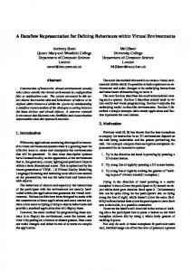
main → reverse ((:)main1 x ((:)main2 y []main )) → (reverse ((:)main2 y []main ) ++ ((:)rev x []rev2 )){(:)main1 → rev} → ((reverse []main ++ ((:)rev y []rev2 )){(:)main2 → rev} ++ ((:)rev x []rev2 )){(:)main1 → rev} main → rev} → (([]{[] ++ ((:)rev y []rev2 )){(:)main2 → rev} ++ ((:)rev x []rev2 )){(:)main1 → rev} rev1

→ (((:)rev y []rev2 ){(:)main2 → rev, []main → rev, []rev1 → ++} ++ ((:)rev x []rev2 )){(:)main1 → rev} → ((:)++ y ([]rev2 ++ ((:)rev x []rev2 ))){(:)main1 → rev, (:)main2 → rev, []main → rev, []rev1 → ++, (:)rev → ++} → ((:)++ y ((:)rev x []rev2 ){[]rev2 → ++} ){(:)main1 → rev, (:)main2 → rev, []main → rev, []rev1 → ++, (:)rev → ++} Figure 1. Computation of Data Flow for reverse [x,y] In the previous examples, we have observed the data flow that is caused by specific applications of reverse. However, we are interested in the flow of data that can be caused by any call to reverse. Therefore, we apply reverse to an unknown value, i.e., a free variable, and observe which constructors in the program flow to which case expressions. We execute the program in a Curry environment in order to get support for unknown values for free. The results are depicted in Table 1. We refer to the constructors introduced by reverse as []rev1 , []rev2 and (:)rev and the constructor introduced by (++) as (:)++ . We refer to the case expressions of the functions as rev and + +. An introduced constructor c and a case expression e where c is matched form a def-use chain denoted by c → e. For def-use chains, only constructors introduced in the program are considered, i.e., constructors that are part of the initial expression do not contribute to the data flow of a program. We can observe that none of the constructors introduced in the program is matched by reverse and all are matched by (++). It may be surprising that even the constructor (:) introduced by (++) can be matched by (++) itself. The reason is that (:)++ is the result of a call to reverse to a list with at least two elements and, therefore, it flows to the first argument of (++) in a call to reverse to a list with at least three elements. 3.2

Functions Flow to Applications

Another source for data flow in declarative programs are higherorder functions. Partial applications flow through a program like constructed terms and, therefore, we treat them as data too. The difference is that functions are not matched in case expressions but applied. Hence, we also refer to a pair of a partial application and an occurrence of an application where the partially applied function or constructor can be applied as def-use chain. Consider the following, more efficient, implementation of the reverse function: rev_linear :: [a] -> [a] rev_linear l = foldl (flip (:)) [] l foldl :: (b -> a -> b) -> b -> [a] -> b foldl op e l = case l of [] -> e (x:xs) -> foldl op (op e x) xs flip :: (a -> b -> c) -> b -> a -> c flip f x y = f y x

Apart from the constructors the definition of rev introduces two partial applications – to (:) and to flip. When rev is applied to a non-empty list the partial application of (:) to zero arguments flows to the application of f to y and x in the definition of flip. The partial application of flip to the argument (:) flows to the application of op to e and x in the definition of foldl.

4.

Monitoring Data Flow

We have implemented the collection of data flow as a program transformation in a test case generator named CyCoTest3 for Curry Coverage Tester. The transformed program computes (along with the original result) a set of def-use chains which represents the data flow caused by the corresponding computation. The transformed program does not use impure features like side effects and preserves the laziness of the original program, i.e., every expression in the transformed program is only evaluated as much as it would be in a corresponding execution of the original program. In (Fischer and Kuchen 2007) we have shown how to employ narrowing to generate test cases for Curry programs. Basically, the tested function is called with logic variables as input that are narrowed during the computation of non-deterministic results. Instead of logic variables, user defined generator functions can be used that compute test input non-deterministically. We have also shown how to collect information w.r.t. control-flow coverage during the execution of a Curry program without using impure features or destroying laziness. We have enhanced this transformation to collect dataflow information as well. However, we only show how to collect def-use chains here – the combination with control-flow coverage is straightforward. We have simplified the transformation presented in (Fischer and Kuchen 2007) by generating lambda expressions and calls to higher-order auxiliary functions. Lambda expressions are not supported by the intermediate language we use. For this description, however, we assume that lambda expressions are available. In our implementation we eliminate them by lambda lifting. 4.1

Attaching Coverage Information

In order to collect the data flow of a computation we attach coverage information to the computed values. Figure 1 shows step-bystep the evaluation of main defined as follows4 : main = reverse [x,y]

We give a subscript to every constructor in the program in order to distinguish different occurrences of the same constructor. The data flow of a computation is denoted by a superscript to corresponding expressions: a set of def-use chains that is attached to an expression denotes exactly those def-use chains that belong to the computation of its head-normal form. After the unfolding of main, the initial call to reverse is unfolded. In this call, the first occurrence of the constructor (:) in function main is matched by reverse. This data flow is denoted as (:)main1 → rev and attached to the result of the unfolding. The next step is again an unfolding of reverse. In this call the second occurrence (:)main2 of (:) in main is matched and we attach 3 pronounced 4x

like psycho test and y denote arbitrary values

Program

P

::=

D1 . . . Dm

Definition

D

::=

f x1 . . . xn = e

Expression

e

::= | | | | |

x c e1 . . . ek f e1 . . . ek let {x1 /e1 ; . . . ; xk /ek } in e case x of {p1 → e1 ; . . . ; pk → ek } apply e1 e2

Pattern

p

::=

c x1 . . . xn

(variable) (constructor call) (function call) (local declarations) (case distinction) (application)

Figure 2. Syntax of Functional Programs the corresponding data flow to the result of the unfolding. In its last recursive call reverse is applied to the empty list []main introduced in the right-hand side of main. The result of this call is the first occurrence []rev1 of [] in reverse and we attach the corresponding data flow []main → rev. The empty list that was the result of the previous call is now matched in a call to the function (++). Note that the matched value []rev1 has an attached defuse chain []main → rev and that we attach this def-use chain to the result of the call to (++). Additionally, the new def-use chain + is recorded. The result of this call is again matched in []rev1 → + a call to (++) and, again, we attach the coverage information of the matched value to the result of the call and record the new def-use chain (:)rev → + +. Now the computation to head-normal form is finished and the data flow caused by this computation is attached to the computed head-normal form. If we continue computing underneath the top-level constructor (:)++ , there is one step left that unfolds the last call to (++). The data flow []rev → + + that is caused by this call is attached to the singleton list underneath the top-level constructor (:)++ . Attaching coverage information to each sub term individually allows to collect data flow of lazy computations. For example, if the tail of the resulting list would be discarded, e.g. by projecting to the head, the def-use chain []rev2 → + + would be discarded as well. In the remainder of this section we discuss the program transformation that allows to compute coverage information as indicated by the example derivation. We first describe our transformation using examples in Subsection 4.2, formalize it in Subsection 4.3, and give the implementation of introduced auxiliary functions in Subsection 4.4. 4.2

Program Transformation

To collect def-use chains, we extend every value of type a to a value of type CyCo a with attached coverage information. As an example, consider the transformed version of the append function (++). (++) :: CyCo [a] -> CyCo [a] -> CyCo [a] l ++ ys = match "++" l (\l’ -> case l’ of [] -> branch0 l ys (x’:xs’) -> branch2 l x’ xs’ (\x xs -> applyCons (applyCons (cons "(:)-app" (:)) x) (xs ++ ys)))

The original type [a] -> [a] -> [a] is adapted to reflect that the transformed function operates on values with attached coverage information. The original definition of (++) performs a matching on its first argument l. The transformed version first calls the auxiliary function match with the following type: match :: ID -> CyCo a -> (a -> CyCo b) -> CyCo b

This function extracts the original value from the extended value and passes it as an argument to the function supplied as second argument. The first argument of type ID is a unique identifier for the corresponding case expression. In our examples, we assume type ID = String. We will discuss the implementation of all auxiliary functions in detail in Subsection 4.4. The branches of the case expression are wrapped with a call to another auxiliary function branchn where n is the number of argument variables in the corresponding pattern. As an example, consider the type of the function branch2: branch2 :: CyCo a -> a1 -> a2 -> (CyCo a1 -> CyCo a2 -> CyCo b) -> CyCo b

This function takes the matched value of type CyCo a and the arguments of the matched constructor of types a1 and a2 and passes extended values of types CyCo a1 and CyCo a2 to the function supplied as last argument. The extended argument values are constructed from the original argument values and corresponding coverage information that is stored with the matched value. The call of the constructor (:) in the second branch of (++) is transformed into combined calls of the auxiliary functions cons and applyCons. All constructor applications are transformed using these functions in order to create representations of complex values extended with coverage information. The types of cons and applyCons are defined as follows: cons :: ID -> a -> CyCo a applyCons :: CyCo (a -> b) -> CyCo a -> CyCo b

The first parameter of cons is a unique identifier for the corresponding occurrence of the supplied constructor. The function reverse is transformed similarly: reverse :: CyCo [a] -> CyCo [a] reverse l = match "rev" l (\l’ -> case l’ of [] -> branch0 l (cons "[]-rev1" []) (x’:xs’) -> branch2 l x’ xs’ (\x xs -> reverse xs ++ applyCons (applyCons (cons "(:)-rev" (:)) x) (cons "[]-rev2" [])))

Note that the function (++) is applied directly in the second branch of the case expression. In contrast to constructor applications, no auxiliary functions are necessary for function applications because functions already take extended values as arguments. With these definitions we can collect the def-use chains depicted in Table 1. 4.3

Formalization

In this subsection, we formalize our program transformation as mapping on programs written in the syntax depicted in Figure 2.

Function- and constructor applications need not be fully applied but must not be over applied, i.e., the number of supplied arguments in a function call f e1 . . . ek must be less or equal to the number of arguments in the definition of the function f . Furthermore, arguments of case expressions are always variables, and patterns in case expressions are flat, i.e., all arguments of the matched constructor are also variables. This representation may seem unnecessarily complex because function- and constructor applications can be written either with or without using apply. On the other hand, the reader may miss lambda expressions. We have chosen this representation because it allows us to discuss first-order programs in isolation before considering the extension to higher-order functions. Lambda expressions can be replaced by partial applications of newly introduced functions using lambda lifting. Hence, we do not consider them in our program transformation. Local declarations cannot be lifted if they are recursive. Hence, we keep them in our language. In a first step, we will assume that all function- and constructor applications are fully applied and that the program does not contain any occurrence of apply. In a second step, we will drop these assumptions and describe the transformation of arbitrary applications and partially applied functions and constructors. Each function of a program is transformed into another function by applying a mapping τ to its body. We have already seen that the most interesting part of the transformation of first-order programs is concerned with constructor applications and case expressions. In fact, everything else is left unchanged: τ (x) = x τ (f e1 . . . ek ) = f τ (e1 ) . . . τ (ek )

(x variable) (f function)

τ (let {x1 /e1 ; . . . ; xk /ek } in e) = let {x1 /τ (e1 ); . . . ; xk /τ (ek )} in τ (e) Constructor applications are transformed using the auxiliary functions cons and applyCons: τ (c e1 . . . ek ) = applyCons(. . . (applyCons (cons c c) τ (e1 )) . . . ) τ (ek ) Note that a constructor c without arguments is just represented as (cons c c). Here, c denotes a unique identifier of this occurrence of the constructor c. The transformation of case expressions introduces calls to the auxiliary functions match and branchn . τ (case x of {. . . (ci xi1 . . . xin ) → ei ; . . .}) = match case x (λ x0 → case x0 of {. . . ci x0i1 . . . x0in → branchn x x0i1 . . . x0in (λ xi1 . . . xin → τ (ei )); . . .}) Here, x0 , x0i1 , . . . , x0in are fresh variable names. Although we did not include lambda expressions in the syntax of our language we use them here to enhance readability. They can easily be eliminated by lambda lifting. The transformation of a case expression applies the auxiliary function match to a unique label case for the case expression, the matched variable x and a lambda expression that introduces a fresh variable x0 . In the original case expression all pattern variables xik are renamed to fresh variables x0ik and passed – along with x – to the auxiliary function branchn . The original pattern variables xi1 , . . . , xin are used as variables in the lambda expression that is also passed to branchn . Hence, we do not need to rename variables in the right-hand sides ei of the case branches. The transformation described so far assumes a first-order program, i.e., all function- and constructor applications are fully applied and there are no occurrences of apply. We now describe the

transformation of arbitrary applications and partially applied functions and constructors. An expression of the form apply e1 e2 is transformed using the auxiliary function applyPartCall: τ (apply e1 e2 ) = applyPartCall apply τ (e1 ) τ (e2 ) Here, apply is a unique identifier for the transformed application. A partial function application is transformed using the auxiliary function partCallm where m is the number of missing arguments. This number can be calculated from the arity of the function and the number of supplied arguments. The arity of a function is the number of argument variables in its definition. The function application f e1 . . . ek where f is a function of arity k + m is transformed as follows: τ (f e1 . . . ek ) = partCallm pm . . . p1 (f τ (e1 ) . . . τ (ek )) Here, p1 , . . . , pm are m unique identifiers for the different parts of this partial application. As partCall0 is the identity function (see Subsection 4.4) the new rule for transforming function applications is a generalization of the rule given before. For the transformation of partial constructor applications, we additionally need the auxiliary function partConsm where m is the number of missing arguments. The constructor application c e1 . . . ek where c is a constructor of arity k + m is transformed as follows: τ (c e1 . . . ek ) = partCallm pm . . . p1 (partConsm (applyCons(. . . (applyCons(cons p0 c) τ (e1 )) . . . ) τ (ek ))) Here, p0 , . . . , pm are m + 1 unique identifiers for the different parts of this partial application. As both partCall0 and partCons0 are the identity function (see Subsection 4.4) the new rule for transforming constructor applications is a generalization of the rule given before. The presented program transformation for higher-order functional programs can be directly translated into an implementation. Interestingly, the transformation can be extended to functionallogic programs in a straightforward way. We have implemented this extension, which is, however, not in the scope of the present paper. 4.4

Implementation

The program transformation presented in the previous subsections introduces calls to auxiliary functions that operate on values of type CyCo a. In this subsection we discuss the implementation of all used data types and functions. We have included different coverage criteria in our implementation but only describe the part that is relevant w.r.t. data-flow coverage. The type CyCo a is defined as follows: data CyCo a = CyCo CyCoTree a data CyCoTree = CCT ID Coverage [CyCoTree]

The type CyCo a associates an unranked tree of type CyCoTree to a value of type a. The structure of this tree reflects the structure of the corresponding data-term. If the original value is a partial function application, the associated tree will have no children. We assume an abstract data type Coverage with the following interface: noCoverage :: Coverage addDataFlow :: ID -> ID -> Coverage -> Coverage mergeCoverage :: Coverage -> Coverage -> Coverage

We do not discuss the implementation of this interface. It is straightforward to implement a set of def-use chains using efficient, purely functional implementations of map data structures. To understand the correspondence between the structure of a value and its associated tree of information we discuss the implementation of the functions cons and applyCons first. The function cons attaches a tree with the given identifier, no coverage, and no children to the given value. cons :: ID -> a -> CyCo a cons i x = CyCo (CCT i noCoverage []) x

The identifier i uniquely identifies the constructor x. The function applyCons is used to apply a wrapped constructor and build complex terms with attached information: applyCons :: CyCo (a -> b) -> CyCo a -> CyCo b applyCons cf cx = CyCo (CCT i cov (t:ts)) (f x) where CyCo (CCT i cov ts) f = cf CyCo t x = cx

The wrapped constructor and argument are selected by pattern matching in a local declaration. The result of applyCons is constructed from the application of the constructor to its argument and a new tree of type CyCoTree. The new tree is identical to the tree that was associated to the constructor before but has an additional child tree – the one that was associated to the argument. We extend the list of child trees at the head to achieve constant run time. Hence, the trees of information that correspond to the arguments of a constructor appear in reverse order. As an example for a complex term with associated information consider the following expression: applyCons (applyCons (cons "c1" (:)) (cons "t" True)) (applyCons (applyCons (cons "c2" (:)) (cons "f" False)) (cons "n" []))

This expression is equivalent to: CyCo (CCT "c1" noCoverage [CCT "c2" noCoverage [CCT "n" noCoverage [] ,CCT "f" noCoverage []] ,CCT "t" noCoverage []]) [True,False]

The shown tree of type CyCoTree reflects the structure of the value (:) True ((:) False []), i.e., [True,False] where arguments appear in reverse order. The unique identifier for each constructor can be found at a corresponding position in the tree and, initially, no coverage information has been collected. Every case expression is transformed using the function match which is defined as follows: match :: ID -> CyCo a -> (a -> CyCo b) -> CyCo b match use (CyCo (CCT def xcov _) x) f = cover (f x) where cover (CyCo (CCT i ycov ts) y) = CyCo (CCT i (addDataFlow def use (mergeCoverage xcov ycov)) ts) y

The function match selects the originally matched value x from its wrapped representation and provides it as an argument to the function f. The coverage information associated with the result of this call is updated twice: • the coverage associated with the top-most constructor of the

matched value is added to the coverage of the result, and • the def-use chain for the corresponding matching is included.

We need to collect the coverage of the top-most constructor because its evaluation is demanded by the case expression for the computation of the result. The function match lies at the heart of our program transformation because here, data flow is monitored. Moreover, this implementation carefully merges exactly the coverage information of a lazy computation without modifying the laziness of the original program (see Fischer and Kuchen (2007) for a detailed discussion of laziness). A careful reader might have noticed that the trees associated to the arguments of the top-most constructor of the matched value are ignored by match. These trees are attached to the corresponding arguments by a call to the function branchn in each branch of a case expression. As an example, consider the implementation of branch2: branch2 :: CyCo a -> a1 -> a2 -> (CyCo a1 -> CyCo a2 -> CyCo b) -> CyCo b branch2 (CyCo (CCT _ _ [t2,t1]) _) x1 x2 f = f (CyCo t1 x1) (CyCo t2 x2)

Note that the argument trees are stored in reverse order in the tree that is associated to the matched value. The given implementation of the used data types and functions suffices to monitor data-flow coverage of first-order functional programs without using side effects. We have implemented support for higher-order functional-logic programs and continue with the description of our treatment of higher-order functions. The extension to free variables and non-determinism, i.e. logic programming, is orthogonal and not in the scope of the present paper. The program transformation presented in Subsection 4.3 introduces calls to auxiliary functions applyPartCall, partConsm , and partCallm which we discuss in the remainder of this subsection. The function applyPartCall is used to apply a wrapped partial application to another argument: applyPartCall :: ID -> CyCo (CyCo a -> CyCo b) -> CyCo a -> CyCo b applyPartCall use cf cx = CyCo (CCT i (addDataFlow def use (mergeCoverage fcov ycov)) ts) y where CyCo (CCT def fcov []) f = cf CyCo (CCT i ycov ts) y = f cx

The function applyPartCall selects the partially applied function from its wrapped representation and applies it to the wrapped argument. The coverage information of the result is updated twice: • the coverage associated with the partial application is added to

the coverage of the result, and • a def-use chain from the partial application to the position

where it is applied is included. The coverage information associated with the partial application needs to be added to the coverage information of the result because an application demands the evaluation of its left argument. We treat partial applications as data and consider the flow of a partially applied function or constructor to its application as data flow. The transformation of partially applied constructors introduces a call to the auxiliary function partConsm . As an example, we discuss the implementation of partCons2: partCons2 :: CyCo (a -> b -> c) -> CyCo a -> CyCo b -> CyCo c partCons2 c x y = applyCons (applyCons c x) y

The function partCons2 takes a wrapped constructor and employs the function applyCons to transform it into a function on wrapped arguments. Note that we can stepwise eliminate the arguments of this definition as follows:

partCons c x = applyCons (applyCons c x) partCons c = applyCons . applyCons c partCons = (applyCons .) . applyCons

Hence, we do not need to provide a definition for partCons2 but can use the right-hand side of the final definition directly in the program transformation. A similar transformation to point-free style is possible for arbitrary m and we do not need to provide a definition for any partConsm function. Finally, we discuss the implementation of partCallm – again exemplified for m = 2: partCall2 :: ID -> ID -> (CyCo a -> CyCo b -> CyCo c) -> CyCo (CyCo a -> CyCo (CyCo b -> CyCo c)) partCall2 i1 i2 f = cons i2 (\a -> cons i1 (\b -> f a b))

The function partCall2 takes two identifiers and a binary function on wrapped arguments and transforms it into a wrapped representation of the partial application that can be applied using applyPartCall. Again, we can stepwise eliminate arguments in this definition: partCall2 i1 i2 f = cons i2 (\a -> cons i1 (f a)) partCall2 i1 i2 f = cons i2 (cons i1 . f) partCall2 i1 i2 = cons i2 . (cons i1 .)

A similar transformation is possible for arbitrary m and we do not need to provide a definition for any partCallm function. Instead of a call to partCallm we can introduce the right-hand side of the final definition in the program transformation – with fresh identifiers as arguments of cons. Apart from free variables and non-determinism we have extended our implementation to primitive functions as well. Although this extension is crucial in order to apply our tool to realistic programs it is of little interest from a research perspective. Therefore, we do not discuss primitive operations in the present paper.

5.

Experiments

We have integrated the described program transformation in our tool for test-case generation. The tool uses narrowing to bind initially uninstantiated input of a tested operation. Alternatively, the user can provide custom input generators – see (Fischer and Kuchen 2007) for details. Let us now have a look how the test-case generator works for some examples. We have selected these examples according to the main application area of the tool, namely glass-box testing of algorithmically challenging units. A unit is in our case a module or a considered function inside of a module. In some cases, we have tested a unit in combination with up to three other units. This corresponds to (small scale) integration testing. It requires more run time, but nevertheless it can be handled. As usual, glass-box unit testing would have to be combined with black-box testing for large-scale integration testing or system testing. However, this is out of the scope of the present paper. The considered examples all contain non-trivial algorithms which makes it hard to cover every relevant behavior by black-box testing. Glass-box testing will ensure that all items corresponding to the considered criterion will be covered. The following example applications have been taken into account. The full source code of all examples as well as the corresponding outputs of our tool can be found at (Kuchen and Fischer 2008). We have introduced an error into each of these examples and we have checked which of the considered coverage criteria is able to expose it. These errors range from deep algorithmic errors (in AVL tree, Dijkstra algorithm, and Kruskal algorithm) based on an insufficient understanding of the application problem to oversights such as switched arguments and wrongly selected operations (e.g.

mod instead of div). The latter usually cause many test cases to expose them. Thus, each of the considered coverage criteria typically has no problems to cover the errors. Tiny test cases will be sufficient here. For some deep algorithmic errors few sophisticated test cases are able to expose them. Thus, the different coverage criteria have more problems to detect the errors. However, even in such situations relatively small counter-examples producing data structures (trees, graphs, heaps, . . . ) of say 4 or 5 nodes are almost always sufficient. This is the reason why our approach works at all in practice. 5.1 5.1.1

Example Applications AVL tree

The well-known AVL tree is a height-balanced binary search tree of logarithmic height (in the number of nodes) (Cormen et al. 1990). This property is ensured by a few restructuring operations, so called rotations. Several of the following example applications (namely Dijkstra, Kruskal, and dynamic programming) use AVL trees as auxiliary data structures for storing tables. The buggy operation insert does not propagate the information on whether the tree has grown correctly. We have introduced another error into the operation delete in the part that handles re-balancing after deletion. Both errors really occurred in our implementation of AVL trees. 5.1.2

Heap

The heap is a classical data structure for storing a priority queue. The declarative variant considered here has been taken from a standard textbook on declarative algorithms (Rabhi and Lapalme 1999). Heaps are used as an auxiliary data structure in the Heapsort and Dijkstra algorithms sketched below. We have investigated the operations insert and delete. In both cases, a simple oversight error has been inserted based on confused arguments in the auxiliary operation merge. 5.1.3

Heapsort

The classical Heapsort algorithm (Cormen et al. 1990) uses the (non-erroneous) heap as an auxiliary data structure. Our implementation contains a simple oversight. 5.1.4

Strassen algorithm

The Strassen algorithm is a well-known divide and conquer algorithm for matrix multiplication. In order to multiply two n × n matrices, it performs seven multiplications of n/2 × n/2 sub-matrices and adds and subtracts the intermediate results in a tricky way (Cormen et al. 1990). The interesting aspect of this example is that it is the only example we found where small test cases are not sufficient in order to expose the error. The reason is that the algorithm for efficiency reasons uses the classical school method for multiplying matrices up to size 16 × 16. The divide and conquer approach is only used for bigger matrices. For our tool this means that a test case which is able to expose an error in the combination of the intermediate results (as we have introduced here) has to include two matrices of sizes 32 × 32 at least. The space of such matrices is that huge that our tool is not able to handle it. However, there is a technique which allows us to tackle even such applications. The problem of our Strassen example is that it contains a hard-coded numerical constant, namely 8 (i.e. 16/2), for recursion control (see (Kuchen and Fischer 2008)). The key idea to handle this problem is to replace the constant by a parameter. With this constant parametrization technique, our tool is able to try small numbers for the parameter. In the case of the Strassen algorithm, 2 × 2 matrices are now sufficient in order to expose the error.

5.1.5

Dijkstra algorithm

The Dijkstra algorithm is a classical approach to compute the distance of every node in a weighted directed graph from some start node (Cormen et al. 1990). The algorithm maintains a heap of border nodes for which upper bounds for their distance to the start node have been computed. In each iteration the node v with the minimal upper bound u is extracted from the heap and moved to the set of finished nodes. Each unfinished neighbor v 0 of v is inserted into the border heap with the sum of u and the length of the edge from v to v 0 as new upper bound. Our implementation uses, in addition to the mentioned heap, (correct) AVL trees for representing weighted directed graphs, node sets, and distance tables. The error we have introduced here is a deep algorithmic one concerning the handling of the border heap. It may cause the same node to be inserted several times into the result table and other nodes to be ignored. Graphs consisting of two nodes are already able to expose this error. 5.1.6

Kruskal algorithm

Kruskal’s algorithm is a classical approach for computing a minimum spanning tree of a weighted undirected graph. The idea is that in each iteration a selected edge is added to the spanning tree. The edge is selected such that it has the minimal weight among all remaining edges not introducing a cycle. A (correct) heap is used to maintain the edges. Moreover, a union-find data structure is used in order to check whether a considered edge would introduce a cycle. Finally, (correct) AVL trees are used to implement sets of nodes as well as tables representing weighted undirected graph. Our implementation is based on the Haskell code found in the textbook by Rabhi and Lapalme (Rabhi and Lapalme 1999). Interestingly, the code in the textbook contains a deep algorithmic error in the use of the union-find data structure which our tool is able to detect. The minimal graph exposing the error consists of 5 nodes. 5.1.7

Dynamic Programming

Another example taken from the mentioned textbook (Rabhi and Lapalme 1999) is a higher-order function for dynamic programming. This function has been used to implement a tabled version of chained matrix multiplications (CMM). The erroneous AVL trees mentioned above are used to represent the required table. In our implementation of CMM, operation div has been erroneously replaced by mod. 5.1.8

Train Ticket

The next example is a computation of the cheapest ticket for the German railway company Deutsche Bahn. After many simplifications of the price structure, the managers of this company have installed a system where the price of a ticket depends on just 16 parameters. Implementing this system leads to a sophisticated branching structure. Some of these branches are executed with very low probability. We have introduced errors into two of these branches. 5.2

Evaluation

Our experiments have been performed on a VMware virtual machine with 700 MB memory running Suse Linux 10.2 on a machine with a 3.6 GHz Xeon processor. We have compared control-flow coverage, data-flow coverage, and a combined control- and dataflow coverage (Table 2). The first coverage approach (CFC) aims at covering all branches of the control-flow graph. It is described in detail in (Fischer and Kuchen 2007). Data-flow coverage (DFC) corresponds to the approach presented in the present paper, while the combined approach (CDFC) tries to cover all branches of the control-flow graph as well as all data flows. For each of the three coverage approaches, we have investigated two coverage scopes. The first of them, Module, only considers

coverable items inside the considered module. The second, Global, also considers control- and/or data-flow between different modules and inside auxiliary modules. In the sequel, a combination of coverage approach and coverage scope will be called coverage criterion. In most Curry implementations the result of a non-deterministic computation can be accessed as search tree that can be processed (lazily) in any order. We have used breadth-first search (BF) as a search strategy for exploring the computation tree in most experiments. The search is stopped, if n test cases have been generated without covering any new items w.r.t. to the considered coverage criterion. If n is chosen sufficiently large, one can be relatively sure that all coverable items will be covered and that the generated test cases really achieve the desired coverage. In most of our experiments we have used n = 200. This is often a very conservative choice. With smaller n, the run time can be reduced considerably while increasing the risk of missing a coverable item. Fixing n as above only makes sense with BF or similar fair strategies, since BF ensures that the progress in exploring the search space is fairly distributed over the whole breadth of the tree. It would not make sense with depth-first search. BF is efficient as long as there is enough memory. In some cases we have experienced memory problems. For example, for Kruskal with CDFC/Global. Then, either n can be reduced or a less space-consuming search strategy such as iterative deepening (ID) has to be used. In our experiments ID has been less efficient than BF. Thus, we have used BF here. The details of our experiments can be found in Table 2. It shows for each considered example application and coverage criterion: which search strategy has been used, whether the error has been covered (+/-), whether the error has been inside of the search space (+/-, in fact always +), how many test cases have been generated in order to fulfill the considered coverage criterion, how many items (control- or data-flows) have been covered, how long the search has taken (in seconds), and how long the elimination of redundant test-cases (see (Fischer and Kuchen 2007)) has taken (in seconds). If the error is inside the search space, this means that our tool has considered a test case exposing the error. However, it may happen that this test case is deleted during the elimination of redundant test cases, since the considered coverage criterion does not ensure it to be preserved. Except for the coverage criterion, the tool has no means to tell which test cases are relevant or not. As our experiments show and as one might expect, CDFC reaches a better coverage than CFC and DFC, while needing more time (up to a factor of roughly two compared to CFC) and space. If using coverage scope Global, CDFC is able to cover every error in our example applications. With coverage scope Module, CDFC could find the error except for the examples Dijkstra and Kruskal. CFC does not cover the error in Kruskal. In general, DFC requires in most cases more time (up to a factor of roughly two) and space than CFC. Interestingly, DFC/Global is able to expose all introduced errors. Coverage scope Module is often not sufficient. If the controland data-flows of auxiliary modules are taken into account, far more errors can be exposed. The run time of our tool is in almost all cases good or acceptable, namely a few seconds or minutes. Only in the Kruskal example, almost half an hour was needed. But even this is acceptable taking into account that the generation of test cases does not often have to be repeated and that it can be performed in the background while doing other work. As a result of our experiments, we recommend the coverage criterion CDFC/Global. It produces the best coverage and exposes most errors, while the overhead compared to other criteria is acceptable. When comparing our tool to QuickCheck, we note that QC exposes errors as well as CyCoTest in most cases, but in less time (see Table 3). QC typically requires a few seconds only, and it

problem AVL.insert

AVL.delete

heap.insert

heap.delete

Heapsort

Strassen

Dijkstra

Kruskal

tabled CMM

Train Ticket

coverage criterion CFC/Module CFC/Global DFC/Module DFC/Global CDFC/Module CDFC/Global CFC/Module CFC/Global DFC/Module DFC/Global CDFC/Module CDFC/Global CFC/Module CFC/Global DFC/Module DFC/Global CDFC/Module CDFC/Global CFC/Module CFC/Global DFC/Module DFC/Global CDFC/Module CDFC/Global CFC/Module CFC/Global DFC/Module DFC/Global CDFC/Module CDFC/Global CFC/Module CFC/Global DFC/Module DFC/Global CDFC/Module CDFC/Global CFC/Module CFC/Global DFC/Module DFC/Global CDFC/Module CDFC/Global CFC/Module CFC/Global DFC/Module DFC/Global CDFC/Module CDFC/Global CFC/Module CFC/Global DFC/Module DFC/Global CDFC/Module CDFC/Global CFC/Module CFC/Global DFC/Module DFC/Global CDFC/Module CDFC/Global

search strategy BF200 BF200 BF200 BF200 BF200 BF200 BF200 BF200 BF200 BF200 BF200 BF200 BF200 BF200 BF200 BF200 BF200 BF200 BF200 BF200 BF200 BF200 BF200 BF200 BF200 BF200 BF200 BF200 BF200 BF200 BF50 BF50 BF50 BF50 BF50 BF50 BF200 BF200 BF200 BF200 BF200 BF200 BF200 BF200 BF200 BF200 BF200 BF100 BF200 BF200 BF200 BF200 BF200 BF190 BF100 BF100 BF100 BF100 BF100 BF100

error covered + + + + + + + + + + + + + + + + + + + + + + + + + + + + + + + + + + + + + + + + + + + + + + + + + + +

error reached + + + + + + + + + + + + + + + + + + + + + + + + + + + + + + + + + + + + + + + + + + + + + + + + + + + + + + + + + + + +

# test cases 5 9 7 12 8 20 9 9 19 23 24 27 2 8 2 7 5 23 2 8 2 10 4 24 1 6 2 7 5 16 1 4 1 13 2 18 1 6 2 9 2 10 1 4 1 9 1 10 1 2 1 7 1 4 3 3 4 7 5 9

# items covered 25 78 51 165 45+51 165+165 41 88 90 223 77+90 204+223 9 38 10 25 17+10 72+25 9 38 6 25 14+6 76+25 15 47 27 59 31+27 90+63 12 94 6 240 35+6 233+240 7 110 7 192 8+7 202+192 19 161 18 370 22+18 328+370 9 125 3 596 9+3 284+555 19 94 13 445 22+13 248+445

search time (s) 17.8 21.8 29.3 33.8 32.0 45.0 29.2 33.3 47.6 57.5 53.8 70.5 2.8 4.8 2.7 4.1 4.3 8.6 1.1 3.2 1.0 3.2 1.2 4.5 60.2 74.0 104.9 106.3 243.8 234.2 45.8 102.8 46.8 170.3 44.7 198.7 39.0 101.6 37.4 119.6 39.6 140.4 1823.0 2709.0 1782.7 2737.4 1796.5 2539.1 17.4 33.8 17.4 112.9 18.3 73.5 50.0 57.0 56.7 130.7 68.2 194.2

elimination time (s) 0.5 3.6 2.0 10.9 4.4 26.6 1.2 4.4 2.9 16.2 6.7 36.8 0.0 0.5 0.1 0.3 0.4 1.7 0.0 0.3 0.0 0.1 0.1 1.2 0.5 1.7 1.5 4.0 6.4 17.5 0.2 8.4 0.0 31.7 0.7 74.0 0.2 13.7 0.2 23.3 0.4 62.2 0.8 39.1 0.7 127.7 2.3 224.6 0.1 17.5 0.0 364.2 0.2 257.3 0.4 13.2 0.2 193.3 1.1 322.1

Table 2. Experimental results for CFC, DFC, and CDFC for some examples. finds the error in all examples except for the train ticket example. Only for examples containing code which is executed with low probability, QC fails, while our tool succeeds. Classical algorithms found in textbooks typically do not contain such code. For “real world applications”, things are different. Besides the train ticket example, we have started to look at a time keeping application, where QC also fails to find an error in code which is executed with low probability. The number of test cases QC needs to find an error changes with every run. This is caused by the fact that the test cases are generated randomly. However, large numbers in the corresponding

column in Table 3 indicate that QC had some problems to find a counter example. LazySmallCheck (LSC) (Lindblad et al. 2007), the intended “improvement” of QC turned out to behave much worse. It could not find the error in the examples Strassen, Dijkstra, Kruskal, and train ticket. Moreover, the search depth had to be reduced in many examples, since we encountered a stack overflow otherwise. This is true for all examples shown in Table 3 where a smaller search depth than 7 was used. In these cases, we have selected the maximal possible search depth. Note that this maximal depth is one (!) in the train ticket example.

problem AVL.insert AVL.delete heap.insert heap.delete Heapsort Strassen Dijkstra Kruskal tabled CMM train ticket

error found + + + + + + + + + -

QuickCheck reductions 25677 1562930 38602 67837 5841 18635 107566 265340 295313 108356190

tests needed 3 45 7 15 5 2 9 13 2 -

LazySmallCheck error reductions depth found + 89224 7 + 3723612 4 + 20294 7 + 12017 7 + 1461 7 2131847 4 2488368 3 1378440 3 + 82427 10 1282008 1

Table 3. Experimental results for QuickCheck and LazySmallCheck. SparseCheck (Naylor 2007), the other “improvement” of QC, turned out to be not mature enough for serious tests. For instance, it cannot handle negative numbers. Since negative numbers are required in most of our examples, we could not include SparseCheck in our comparison.

6.

Conclusions and Future Work

Reliable testing of declarative programs gains importance as they are used to develop main stream applications. Currently, QuickCheck (Claessen and Hughes 2000) is used in combination with Haskell Program Coverage (Gill and Runciman 2007) to evaluate the quality of tests for the window manager Xmonad (Stewart and Sjanssen 2007). HPC is quite efficient and very useful despite its simple coverage criterion. However, 100% coverage does not always mean that the program is tested thoroughly enough. We have developed a tool that generates a minimal set of test cases w.r.t. different coverage criteria. In the present paper, we have introduced a novel notion of data-flow coverage for declarative programs to improve the quality of test cases selected by our tool. The data flow caused by the execution of a program is a set of defuse chains. There are two different kinds of def-use chains: • constructors flow to case expressions, and • functions flow to applications.

We have presented a program transformation that instruments declarative programs such that they compute the data flow of their execution along with the original result. The generated program is a purely functional program – it does not use any side effects to monitor coverage. An extended version of this transformation is integrated into our test tool, which allows to generate minimal sets of test cases w.r.t. control and/or data flow. We have simplified the program transformation presented previously (Fischer and Kuchen 2007) and provide a detailed description of the treatment of higher-order functions in the present paper. We usually execute the transformed program with logic variables as input to generate test cases. However, it can also be executed on ground values generated beforehand in order to compute coverage information for a specific program run. The advantage of using narrowing for test-case generation is that the input is instantiated according to the program’s demand which is what makes our tool a glass-box tool. A set of test cases that are instantiated exactly as demanded by the computation is more likely to induce the possible code coverage compared to test cases that are generated without taking the structure of the program into account. Instead of logic variables, user defined generator functions can be used to compute test input non-deterministically. This allows to generate data terms with additional constraints on their structure like, e.g.,

AVL trees. As Curry cannot guess values of functional type, user defined generators are mandatory in order to generate higher-order test data. Test cases for higher-order programs without functions as input can be generated without user defined generators. Coverage-based testing is especially useful for algorithmically complex program units. We have selected a couple of such examples and compared the quality of selected tests using different coverage criteria. For this purpose, we have introduced a bug in each example and checked whether this bug was exposed by the generated minimal set of test cases. It turns out that data-flow coverage improves the quality of the generated tests and that most thorough testing is achieved by a combination of control and data flow. During our experiments, our tool has exposed a subtle error in the description of Kruskal’s minimum spanning tree algorithm given in a textbook by Rabhi and Lapalme (1999). When comparing our tool with existing tools for Haskell, it turns out that black-box testing with QuickCheck is surprisingly effective as long as the programmer provides good input generators. Glass-box testing is more effective than black-box testing only for programs containing parts that are executed with low probability. The pricing system of the German railway company is an example for such an application. There are different directions for future work, e.g., 1. adaptive search, 2. coverage visualization, and 3. automatic bug location. Adaptive Search In the current implementation we use breadthfirst search or iterative deepening depth-first search to generate test cases. Both strategies blindly enumerate the search space. Curry allows to enumerate the search space with user-defined functions, hence, it is possible to guide the search using coverage information. Based on the coverage of previously found test cases, the enumeration function can estimate where it is most likely to find test cases that cause new coverage. Coverage Visualization Currently, we use coverage information only to reduce the number of test cases. A visual representation of control- and/or data flow would help the user to understand the executions of the program. This is especially useful for the execution of a test case that exposes an error. Automatic Bug Location By comparing the coverage of successful and failing test cases, one can pinpoint parts of the program that are executed often in buggy computations and seldom in correct ones. This would allow to distinguish parts that are likely to contain a bug from other parts that are likely to be correct. Such information could significantly simplify the process of finding bugs in algorithmically complex programs.

References Elvira Albert, Miguel G´omez-Zamalloa, Laurent Hubert, and Germ´an Puebla. Verification of Java bytecode using analysis and transformation of logic programs. In Proc. PADL, LNCS 4354, pages 124–139, 2007. B. Beizer. Black-Box Testing. Wiley, 1995. Olaf Chitil, Colin Runciman, and Malcolm Wallace. Transforming Haskell for tracing. In Ricardo Pena and Thomas Arts, editors, Implementation of Functional Languages: 14th International Workshop, IFL 2002, LNCS 2670, pages 165–181, March 2003. ISBN 3-540-401903. URL http://www.cs.kent.ac.uk/pubs/2003/1770. Madrid, Spain, 16–18 September 2002. Jan Christiansen and Sebastian Fischer. EasyCheck – test data for free. In FLOPS ’08: Proceedings of the 9th International Symposium on Functional and Logic Programming. Springer LNCS 4989, 2008. Koen Claessen and John Hughes. Quickcheck: a lightweight tool for random testing of Haskell programs. In Proc. ICFP, pages 268–279, 2000. T.H. Cormen, C.E. Leiserson, and R.L. Rivest. Introduction to Algorithms. McGraw Hill, 1990. Sebastian Fischer and Herbert Kuchen. Systematic generation of glass-box test cases for functional logic programs. In Proc. of the 9th International ACM SIGPLAN Symposium on Principles and Practice of Declarative Programming (PPDP 2007), pages 75–89. ACM Press, 2007. Andy Gill and Colin Runciman. Haskell program coverage. In Haskell ’07: Proceedings of the ACM SIGPLAN workshop on Haskell workshop, pages 1–12, New York, NY, USA, 2007. ACM. ISBN 978-1-59593-6745. M.

Hanus et al. Curry: An integrated functional logic language (version 0.8.2). Available at URL http://www.informatik.uni-kiel.de/~curry, 2006.

Pieter W. M. Koopman, Artem Alimarine, Jan Tretmans, and Marinus J. Plasmeijer. Gast: Generic automated software testing. In Proc. IFL, LNCS 2670, pages 84–100, 2002. H. Kuchen and S. Fischer. CyTest benchmarks web pages. URL http://danae.uni-muenster.de/lehre/kuchen/ICFP08/, 2008. Fredrik Lindblad, Matthew Naylor, and Colin Runciman. A logic programming library for test-data generation. Available at http://www-users.cs.york.ac.uk/~mfn/lazysmallcheck/, 2007. Roger A. M¨uller, Christoph Lembeck, and Herbert Kuchen. A symbolic Java virtual machine for test-case generation. In IASTED Conf. on Software Engineering, pages 365–371, 2004. N. Mweze and W. Vanhoof. Automatic generation of test inputs for Mercury programs. In Proc. LOPSTR, 2006. Matthew Naylor. A logic programming library for test-data generation. Available at http://www-users.cs.york.ac.uk/~mfn/sparsecheck/, 2007. S. Peyton Jones, editor. Haskell 98 Language and Libraries—The Revised Report. Cambridge University Press, 2003. F. Rabhi and G. Lapalme. Algorithms – A Functional Programming Approach. Addison Wesley, 1999. Don Stewart and Spencer Sjanssen. Xmonad. In Haskell ’07: Proceedings of the ACM SIGPLAN workshop on Haskell workshop, pages 119–119, New York, NY, USA, 2007. ACM. ISBN 978-1-59593-674-5.