DATA-INTENSIVE COMPUTING FOR BIOINFORMATICS USING VIRTUALIZATION TECHNOLOGIES AND HPC INFRASTRUCTURES
A Thesis Presented to the Graduate School of Clemson University
In Partial Fulfillment of the Requirements for the Degree Master of Science School of Computing
by Pengfei Xuan December 2011
Accepted by: Dr. Feng Luo, Committee Chair Dr. Amy W. Apon Dr. Anna V. Blenda
ABSTRACT The bioinformatics applications often involve many computational components and massive data sets, which are very difficult to be deployed on a single computing machine. In this thesis, we designed a data-intensive computing platform for bioinformatics applications using virtualization technologies and high performance computing (HPC) infrastructures with the concept of multi-tier architecture, which can seamlessly integrate the web user interface (presentation tier), scientific workflow (logic tier) and computing infrastructure (data/computing tier). We demonstrated our platform on two bioinformatics projects. First, we redesigned and deployed the cotton marker database (CMD) (http://www.cottonmarker.org), a centralized web portal in the cotton research community, using the Xen-based virtualization solution. To achieve highperformance and scalability for CMD web tools, we hosted the large amounts of protein databases and computational intensive applications of CMD on the Palmetto HPC of Clemson University. Biologists can easily utilize both bioinformatics applications and HPC resources through the CMD website without a background in computer science. Second,
we
developed
a
web
tools
―
Glycan
Array
QSAR
Tool
(http://bci.clemson.edu/tools/glycan_array), to analyze glycan array data. The user interface of this tool was developed at the top of Drupal Content Management Systems (CMS) and the computational part was implemented using MATLAB Compiler Runtime (MCR) module. Our new bioinformatics computing platform enables the rapid deployment of data-intensive bioinformatics applications on HPC and virtualization environment with a user-friendly web interface and bridges the gap between biological scientists and cyberinfrastructure.
ii
ACKNOWLEDGMENTS Foremost, I would like to thank Dr. Anna Blenda, the Principal Investigator of the Cotton Marker Database development (project 03-391 funded by the Cotton Incorporated), for the financial support of my graduate research assistantship and the opportunity to do my research using the CMD resources. In addition, I would like to thank Dr. Blenda for her advice and friendship. One of the primary benefits of working for Dr Blenda is the freedom she has given me to design my own solutions to the CMD project and perform the further exploration of the solutions. I would like to express my sincere gratitude to my advisor, Dr. Feng Luo for the continuous support of my study and research, for his patience, motivation, enthusiasm, and immense knowledge. His guidance helped me in all the time of research and writing of the thesis and papers. His ability to answer fundamental questions about complex problems without losing sight of the grand scheme is an ability that I hope to someday acquire. Dr. Luo has played a large and unique part in helping me reach this point in my journey. I would also like to expressly thank Dr. Amy Apon for being on my committee, reviewing my dissertation and her insight into how to continue my future research. I am very grateful to the remaining members: Dr. Bo Li, Yuehua Zhang, Aditya Sriram and Gauri Jape (BCI research group), Dr. Stephen Ficklin, Dr. Meg Staton and Dr. Chris Saski (CUGI laboratory), Dr. Véronique Decroocq (INRA, France) and Dr. Jean-Marc Lacape (UMR-DAP, France), for their research collaboration, support, and friendship.
iii
Finally, I would like to thank my wife – Yueli Zheng, my daughter – Emma Xuan, my parents Yuhai Xuan and Jingzhen Li, and my mother-in-law Ailian Zhao. I would not have achieved this without their constant love and support.
iv
TABLE OF CONTENTS Page TITLE PAGE ……………………………………………………………………………...i ABSTRACT………………………………………………………………………………ii ACKNOWLEDGEMENT ……………………………………………………………….iii LIST OF TABLES……………………………………………………………………….vii LIST OF FIGURES……………………………………………………………………..viii ACRONYM TABLE…..…………………………………………………………………xi CHAPTER
1
INTRODUCTION ................................................................................................. 1
2
BACKGROUND .................................................................................................. 4 2.1 2.2
Virtualization .................................................................................. 4 Machine Learning ........................................................................... 5 2.2.1 2.2.2 2.2.3
2.3 2.4 2.5 2.6 2.7 3
Classification and Prediction .............................................. 5 Support Vector Machine ..................................................... 6 Evaluation Criteria .............................................................. 7
Partial Least Squares (PLS) Regression ......................................... 9 GMOD .......................................................................................... 10 BLAST and FASTA ..................................................................... 11 BioPerl .......................................................................................... 12 Drupal ........................................................................................... 12
BIOINFORMATICS PLATFORM DESIGN, IMPLEMENTATION AND DEPLOYMENT .................................................................................... 14 3.1 3.2
Multi-tier Architecture .................................................................. 14 Presentation Tier ........................................................................... 17 3.2.1 3.2.2
CMD Web Interface.......................................................... 17 BCI Glycan Array QSAR Tool Interface.......................... 22
v
Table of Contents (Continued) Page 3.3
Logic Tier...................................................................................... 25 3.3.1 3.3.2 3.3.3
3.4
Data / Computing Tier .................................................................. 31 3.4.1 3.4.2
3.5
4
Email System .................................................................... 34 DNS Service...................................................................... 36 Web Analytics................................................................... 36
Server Virtualization ..................................................................... 37 Backup .......................................................................................... 39
COTTON MARKER DATABASE ........................................................................ 42 4.1 4.2 4.3 4.4
Introduction ................................................................................... 42 New SSR Projects ......................................................................... 43 Primer Redundancy Information of SSRs..................................... 45 SSR Redundancy Detection using SVM Machine Learning Approach ................................................. 47 4.4.1 4.4.2
4.5 5
Database System ............................................................... 31 Directory Structure on Palmetto HPC............................... 33
System Services ............................................................................ 34 3.5.1 3.5.2 3.5.3
3.6 3.7
Data Flow on Bioinformatics Platform ............................. 25 CMD Web Tools ............................................................... 26 BCI Glycan Array QSAR Tool ......................................... 30
Materials and Methods...................................................... 47 Result ................................................................................ 49
QTL/Traits Feature and Cotton Genetic Maps ............................. 51
QUANTITATIVE STRUCTURE-ACTIVITY RELATIONSHIP (QSAR) STUDY ON GLYCAN ARRAY DATA .......................................................... 53 5.1 5.2
Introduction ................................................................................... 53 Results ........................................................................................... 55 5.2.1
Coding Glycans using Sub-tree Features .......................... 55
vi
Table of Contents (Continued) Page
5.2.2 PLS Regression on Glycan Array Data using Different Features .............................................. 58 5.2.3 Identification of Significant Structural Features in Glycans ................................................................... 66 5.2.4 Evaluation of QSAR Model on Other Glycan-binding Proteins ............................................. 75 5.3
Discussion ..................................................................................... 81
CHAPTER 6
CONCLUSION AND FUTURE WORK ................................................. 85
APPENDIX A
....................................................................................................... 88
REFERENCES
..................................................................................................... 114
vii
LIST OF TABLES Table
Page 3.1
MX records of CMD mail servers ............................................................... 36
3.2. The network configuration information ....................................................... 39 4.1. The summary of primer redundancy processing .......................................... 46 4.2
The algorithm to select the SSR redundancy training data. ......................... 50
4.3
Evaluation of results obtained for the tested data ........................................ 50
5.1
The R2 of PLS regressions on glycan array data of different glycan-binding proteins using different features. ................................... 62
5.2
The highest R2 of PLS regressions on glycan array data of different glycan-binding proteins. .......................................................... 62
5.3
The significant di-saccharide sub-trees binding specifically to ConA. ....... 71
5.4
The significant di-saccharide sub-trees binding specifically to VVL. ......... 71
5.5
The significant di-saccharide sub-trees binding specifically to WGA. ....... 72
5.6
The significant tri-saccharide sub-trees binding specifically to PNA. ........ 76
5.7
The significant di-saccharide sub-trees binding specifically to SNA. ......... 76
5.8
The significant tri-saccharide sub-trees binding specifically to DC-SIGN. ............................................................................................... 78
5.9
The significant mono-saccharide sub-trees binding specifically to Siglec-8. .................................................................................................. 78
5.1
The R2 of PLS regressions on glycan array data of different antibodies using different features. .......................................................................... 80
5.11 The significant tetra-saccharide sub-trees binding specifically to CSLEX1 (human CD15s antibody). ....................................................... 80 5.12 The significant tetra-saccharide sub-trees binding specifically to Sialyl Lewis x antibody-10. .................................................................... 81
viii
LIST OF FIGURES Figure
Page 2.1
The architecture of virtualization platform .................................................... 5
3.1
The architecture of data-intensive computing platform for bioinformatics applications. .............................................................. 15
3.2
Home page of the CMD. .............................................................................. 18
3.3
The web interface for primer redundancy page ........................................... 19
3.4
CMD Trait View Page. ................................................................................ 22
3.5
CMD CMap Viewer..................................................................................... 22
3.6
The web interface of Glycan Array QSAR Tool. ........................................ 23
3.7
An example result of Glycan Array QSAR Tool. ........................................ 24
3.8
The data flow on Cotton Marker Database. ................................................. 26
3.9
CMD web tools execution workflow. .......................................................... 27
3.10 The Glycan QSAR tool execution workflow. .............................................. 30 3.11 The database schema of CMD website ........................................................ 32 3.12 The directory structure in Palmetto HPC ..................................................... 33 3.13 The management interface of CMD mail list system .................................. 35 3.14 The interface of Google Analytics ............................................................... 37 3.15 Snapshot and rsync backup solution to CMD virtualization platform......... 41 3.16 The structure of backup directory on the remote backup server .................. 41 4.1
The redundant primer counts obtained for each of the individual threshold values ..................................................................... 46
4.2
The SVM machine learning workflow. ....................................................... 48
4.3
ROC curve analysis...................................................................................... 51
ix
List of Figures (Continued) Figure
Page 5.1
An example of glycan chain and its structure. ............................................. 56
5.2
An example of decomposing the glycan chain in into different sub-trees. .................................................................................. 56
5.3
Plot of the percentage of variance explained in the binding intensities of glycan array data of three plant lectins against the number of components in PLS. ........................................................ 60
5.4
Plot of observed intensities against the fitted intensities calculated by PLS regression using di-saccharide sub-trees as features ................. 65
5.5
The distribution of PLS regression coefficients (Beta values) obtained from glycan array data of ConA. ............................................. 67
5.6
The distribution of PLS regression coefficients (Beta values) obtained from glycan array data of VVL. .............................................. 67
5.7
The distribution of PLS regression coefficients (Beta values) obtained from glycan array data of WGA. ............................................. 68
x
ACRONYM TABLE AUC
Area Under Curve
BLAST
Basic Local Alignment Search Tool
BCI
Bioinformatics and Chemical Informatics
CFG
Consortium for Functional Glycomics
CMD
Cotton Marker Database
CMS
Content Management System
EST
Expressed Sequence Tags
GMOD
Generic Model Organism Database
LVM
Logical Volume Manager
LV
Logical Volume
MCR
MATLAB Compiler Runtime
MPI
Message Passing Interface
MX
Mail Exchange
NGS
Next Generation Sequencing
ORFs
Open Reading Frames
PBS
Portable Batch System
PLS
Partial Least Squares
QSAR
Quantitative Structure-activity Relationship
QTL
Quantitative Trait Locus
ROC
Receiver Operating Characteristic
SNP
Single-nucleotide Polymorphism
SSR
Simple Sequence Repeats
SVM
Support Vector Machines
VM
Virtual Machine
xi
Chapter 1 Introduction The bioinformatics application often involves many computational components and a large number of runs with different parameters and configurations [1-4]. Recently, the genomic research based on Next Generation Sequencing (NGS) technology makes it possible to study biological phenomena on a large scale: all metabolic processes in a tissue, all transcripts in a cell, and all genes in a genome. However, sequencing-based genome-wide analysis also products massive quantities of data, which brings a new challenge facing the current bioinformatics research [5] and finally leads to the insufficiency of performance or capability on a local workstation or server. For example, the amount of data from the 1000 Genomes Project [6] will reach the petabyte scale for the raw sequence information. In the near future, the situation will be dramatically changed by third-generation sequencing technologies [7]. It will allow us to scan entire transcriptomes, microbiomes and genomes, and make it possible to assess epigenetic changes directly [8] in a few minutes with the cost less than US$100. Today’s dataintensive biology drives a new emerging computational model to integrate massive data with computing resources derived from molecular biology. Biological research is becoming more and more dependent on big data analysis. Biologists will soon encounter difficulties in handling missive data sets using traditional applications or tools that were initially designed for the single machine or non-dataintensive task in such areas as protein or nucleic acid sequence assembly, sequence
1
alignment for similarity comparisons, motif recognition in linear sequences or higherorder structure, and common patterns of gene expression; Further, while current technologies can provide large-scale computing solutions to analyze, integrate and manipulate big data sets, there still exists a huge knowledge gap for biologists with sufficient computer science background to utilize high-end platform resources. This shortage means biologists have to either avoid research areas relevant to big data sets or collaborate with data scientists. Due to lack of the ability to analyze the massive data, many promising biological projects have to be given up or cannot keep growing in longterm investments, and the ecosystem of bioinformatics research would also be limited to a very small scope. High-performance Computing (HPC) is a typical computing infrastructure that provides high-performance parallel file systems with both high bandwidth and large capacity. Parallel file systems like PVFS [9], HDFS [10], GPFS [11] and Lustre [12] are usually employed to meet these needs and are often layered on top of clustered storage systems or use special high-end customized hardware. These systems are geared towards storing petabyte-scale data in a reliable fashion with high throughput for massive computing jobs. To make the bioinformatics resource and software more accessible, and allow for a faster overall time-to-solution, a user-friendly computing platform based on cyberinfrastructure could be a promising way to lead biologists to a new scientific paradigm: data-driven science. In this thesis, we propose a platform solution for data-intensive bioinformatics applications using virtualization technologies and HPC infrastructures. A multi-tier
2
architecture is used to integrate the web user interface (presentation tier), scientific workflow (logic tier) and computing infrastructure (data/computing tier). The platform has been demonstrated through two bioinformatics projects: One is Cotton Marker Database (CMD) (http://www.cottonmarker.org) which is a centralized web portal in the cotton research community. The other project is a quantitative structure-activity relationship (QSAR) Tool (http://bci.clemson.edu/tools/glycan_array) used to analyze glycan array data. The remainder of this thesis is organized as follows. Chapter 2 provides background and terminology information, including concepts to construct our new bioinformatics computing platform. Chapter 3 gives a detailed solution to design and deploy data-intensive computing platform for bioinformatics applications. Chapter 4 demonstrates the CMD project on HPC and virtualization environment. Chapter 5 shows a glycan array QSAR on our new bioinformatics platform. And finally Chapter 6 offers conclusions and future works.
3
Chapter 2 Background Bioinformatics is an interdisciplinary field that combines aspects of Biology, Mathematics, and Computer Science [13], which are also theoretical foundations of our bioinformatics platform and related projects. In following sections, we introduce several terminologies and concepts in these areas to give a basic background for the further discussions in the remainder chapters.
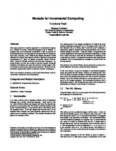
2.1 Virtualization Virtualization is a computing construct for running software (usually operating systems) concurrently and isolated from other programs on a single computer system [14]. Figure 2.1 shows the architecture of a virtualization platform. Typically, the architecture of OS virtualization includes a hypervisor, a software layer or subsystem that controls hardware and provides guest OSs with access to underlying hardware. The hypervisor allows multiple individual guest OSs to share the same physical system by offering virtualized hardware using various approaches (such as, full virtualization, paravirtualization and software virtualization) to mapping [15]. Guest OSs could be 32-bit or 64-bit Windows, Linux or Unix systems, which provides wide support for various applications and services. There are many different types of virtualization platforms, including Xen, KVM, VMware, VirtualBox, OpenVZ and Solaris containers.
4
Figure 2.1 The architecture of virtualization platform In our project, a Xen-based virtualization solution is used to support two product websites. The Xen framework is a very popular and common solution for the Linux platform. The Xen hypervisor contains three components, Domain 0, the Xen Hypervisor and Multiple Domain U [14]. These run directly on top of the physical machine, and act as the middle layer for the guest operating systems to access all hardware such as CPU, I/O, and disk. Domain 0 is the only domain that has privileges to access the Xen hypervisor. These privileges allow Domain 0 to manage and control all Domain Guests (DomUs), including starting, stopping, network requests, and so on.
2.2 Machine Learning 2.2.1 Classification and Prediction Classification, also called supervised learning, is the computational approach of finding a model from training data and predicting the class of testing data. The model built from training data set has the ability to characterize and distinguish prediction data sets with a form of rules, decision tree or mathematical functions. Sample sets are usually observations or measurements labeled with features and class. Features selected for the
5
samples should relate to the classes, and the labels predicted by the classifier are usually categorical. For models generating continuous numerical values, the labels can be obtained by discretization. Some typical classification algorithms are decision tree, random forest, support vector machine and naïve Bayesian. Various approaches can be used to validate the prediction result. The cross validation is one of the common and effective approaches. In this method, the sample data is randomly split into n sets. One set in the middle is used for testing and the other 𝑛 − 1 sets are used for training. Totally n iterations will be conducted, and the average of each result will be calculated to represent the performance.
2.2.2 Support Vector Machine Support Vector Machines (SVM) [16] are a computational method for data classification by constructing a hyperplane (or set of hyperplanes) in a high or infinite dimensional space, which can be used for regression, classification, or other further tasks. The original problem is often stated in a finite dimensional space in which the sets to discriminate are not linearly separable. The principle of SVM is to map the original finite-dimensional space into a much higher-dimensional space to make the separation easier. A hyperplane created by the SVM is based on the largest distance to the nearest training data points of any class (functional margin). To avoid overfitting the problem, a buffer (soft margin) is used to provide certain error tolerances during the training stage. There are many implementations of SVM, such as LibSVM [17], SVMlight [18] and
6
TinySVM [19]. In our project, we use LibSVM tools with different kernel functions to improvement Simple Sequence Repeats (SSR) redundancy of the CMD website.
2.2.3 Evaluation Criteria In order to measure the performance of classification result, multiple criteria were employed including sensitivity, specificity, precision, accuracy and F-measure. Four basic terminologies are used to definite these criteria which are true positive (TP), false positive (FP), true negative (TN) and false negative (FN) respectively. True positive is the correctly predicted positive data. True negative is the correctly predicted negative data. False positive is the predicted positive data that actually belong to the negative class. False negative is the predicted negative data that actually belong to the positive class. The definition of sensitivity, specificity, precision, accuracy and F-measure are shown here, Sensitivity is the probability of correctly predicted positive data over the total number of positive data. Sensitity =
TP
TP+FN
(2.1)
Specificity is the probability of correctly identified negative data over the total number of negative data. Speci�icity =
TN
TN+FN
(2.2)
Precision is the probability of correctly predicted positive data over the total number of predicted positive data. Precision =
7
TP
TP+FP
(2.3)
Accuracy is the probability of correctly predicted positive and negative data over the sum of positive and negative data. Accuracy =
TP+TN
TP+TN+FP+FN
(2.4)
The F-measure or F-score is a measure of the accuracy of testing data by considering both the precision and recall of the test to compute the score. The best Fmeasure score is 1 and the worst F-measure score is 0. F=
2×(Precision×Recall) (Precision+Recall)
(2.5)
Additionally, ROC (Receiver Operating Characteristic) curve and AUC (Area Under Curve) value serve to evaluate the discriminate power of models, and can be used to select the optimal models. ROC curve is used to measure the classifier in the cross validation study and the prediction performance. ROC curve plots the fraction of true positives against the false positive rate as the threshold of prediction varies. ROC evaluates the performance of classifiers based on the tradeoff between specificity and sensitivity. While ROC curve provides a visualization method to evaluate a classifier, AUC (area under the curve) score is widely used by providing a numeric value for the comparison of prediction performance. While an AUC value of 1 means perfect prediction, an area of 0.5 indicates random prediction. Most common models should have AUC values between 0.5 and 1.0. The higher the AUC value, the better the model. High AUC value means that lowering the threshold for the prediction only brings in limited false positive samples.
8
2.3 Partial Least Squares (PLS) Regression The PLS regression has been widely used to model the relationship between responses and predictor variables [20]. For example, responses are the properties of chemical samples and predicator variables are the composition of chemicals. In our study, the response is the binding intensity of glycan chains to glycan-binding proteins and the predictor variables are the sub-trees extracted from glycan chains. Unlike general multiple linear regression, the PLS regression can handle strong collinear data and the data in which number of predictors is larger than the number of observations. The PLS build the relationship between response and predictors through a few latent variables constructed from predictors. The number of latent variables is much smaller than that of the original predictors. Let vector y (n×1) denote the single response; matrix X (n×p) denote the n observations of p predictors and matrix T (n×h) denote n values of the h latent variables. The latent variables are linear combinations of the original predictors:
Tij = ∑ Wkj X ik
(2.6)
k
where matrix W (p×h) is the weights. Then, the response and observations of predictors can be expressed using T as follows [20]: X ik = ∑ Tij Pjk + Eik
(2.7)
y m = ∑ C mj Tij + f m
(2.8)
j
j
where matrix P (h×p) is the is called loadings (the regression coefficients of latent variables T for observations) and matrix C (h×1) is the regression coefficients of T for responses. The matrix E (n×p) and vector f (n×1) are the random errors of X and y. The
9
PLS regression decomposes the X and y simultaneously to find a set of latent variables that explain the covariance between X and y as much as possible [20]. The PLS regression was performed using the plsregress function in Matlab. The plsregress function takes three parameters: X, y and the number of components. It is important to determine the number of components in PLS regression. We employed the following procedure to select the number of components. We first ran the PLS regression using a large number of components, for example, 50. The plsregress returned the percentage of variance explained in response for each PLS component. Then, we counted the number of components that contribute to variance explained beyond a threshold. This number was our new number of components. In our study, we set the threshold to be 0.5% of variance explained. We then ran PLS regression again using the new number of components. The R2 of PLS regression is calculated using the formula: R 2 = SSerr SStotal . The SSerr is the sum of squares of fit errors: SSerr = ∑ f 'i , where f’ (n×1) is the regression i
errors. And the SStotal is the total sum of squares: SStotal = ∑ ( yi − y ) 2 , where y is the i
mean of y.
2.4 GMOD Generic Model Organism Database (GMOD) project, is a collection of open source software tools to create and manage genome-scale biological databases [21]. There are more than 37 components and 14 functionality areas in GMOD project. These components provide the functionality that is needed by all organism databases like Community Annotation, Comparative Genome Visualization, Database schema, Database
10
tools, Gene Expression Visualization, Genome Annotation, Genome Visualization & Editing, Ontology Visualization, Literature Tools, Workflow Management, Molecular Pathway Visualization, Middleware, Tool Integration and Sequence Alignment. In modern biology research area, bioinformatics applications and databases are begin developed at a steady rate. However, many of these tools are seldom used since the user may not have the resources or skills to install the tool and integrate them. There is need for a standardized solution to integrate those tools and databases together. GMOD provides such a platform for developers, scientists and laboratories to construct their own bioinformatics software.
2.5 BLAST and FASTA BLAST (Basic Local Alignment Search Tool) program [22] and FASTA program [23] are both tools for sequence similarity search which can be used to compare a query to a DNA/protein database by a stand-alone tool or a web interface. The difference between BLAST and FASTA is that they use different algorithm for comparison. FASTA is better for less similar sequences. BLAST may be faster than FASTA without significant loss of ability to find the similar sequences in the DNA/protein database. BLAST is one of the most widely used bioinformatics tools. There are several variants of BLAST programs that can compare between protein or nucleotide queries with protein or nucleotide databases.
11
2.6 BioPerl BioPerl is an open-source international project (since 1995) [5] to facilitate sequence alignments, genetic sequence manipulation and genomic analysis. It allows bioinformatieists, genetic researchers and computer scientists to collaboratively focus on providing a set of well-documented Perl modules [24]. It provides a set of foundational libraries that allow the building of complex bioinformatics tools for use in production quality software [4] and the construction of complex solutions to bioinformatics problems. BioPerl (version 1.6.9) gives support to read/write of multiple sequence file formats, sequence retrieval from web databases, sequence manipulation and alignment and sequence annotations.
2.7 Drupal Drupal is one of most widely used open source web Content Management Systems (CMS), which are used to create integrated web sites. Drupal web sites can include a blog, a portal web site for the organization, an e-commerce site, a social networking site and other componets [25]. The framework of the Drupal system is highly modular, extensible, and standards-compliant. The official version of Drupal only contains the basic core functionality, however, additional functionality can be added using built-in or third-party modules. There are more than 9,000 modules available to extend and customize Drupal functionality. To apply these modules does not require any modifications to the code in the core. CMS use in bioinformatics is growing [26]. Drupal is used for many applications, including in on-line analysis tools, intranet tools, collaboration tools, biology databases,
12
conference websites and lab websites. For example, Drupal is selected as the core development framework in GMOD Tripal project [27]. The Tripal modules allow the Drupal CMS to interact with Chado [28] data, as well as provide data loaders, display of Chado data and administrative interfaces for data management. Our glycan array QSAR tool also was developed as a module of Drupal platform by customizing Webform module and Theme module. Detailed discussion will be given at the next chapter.
13
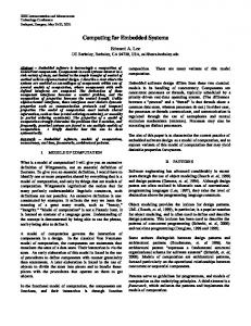
Chapter 3 Bioinformatics Platform Design, Implementation and Deployment In this chapter, we will discuss the design, implementation and deployment of the system platform regarding data-intensive bioinformatics applications. The primary design goal is to create a flexible, configurable and high-performance framework with a userfriendly web interface. Based on the new design, biologists with minimal computer science background can easily analyze massive data sets by using public computing infrastructure. Figure 3.1 shows the architecture of the data-intensive computing platform for bioinformatics applications using virtualization technologies and HPC infrastructures. Detailed description of the multi-tier architecture for the bioinformatics platform is presented in the following sections of the thesis.
3.1 Multi-tier Architecture Our design applies the software engineering concept of multi-tier architecture including presentation tier, logic tier and data/computing tier. It can seamlessly integrate the web user interface, scientific workflow and computing infrastructure (Figure 3.1).
14
Figure 3.1 The architecture of data-intensive computing platform for bioinformatics applications. Presentation tier The presentation tier is the top layer of the platform. The presentation tier provides user-friendly web interface related to various bioinformatics applications, such as tools for sequence alignment in similarity comparisons, protein sequence or nucleic acid assembly, genetic map views, SSR information retrieval, or glycan array data analysis. All computational parameters and input data sets are submitted from this tier, and then initial information is passed to the next tier. The presentation tier includes three services: a form validation service, the CMS service and a search service. The interface of this tier is implemented using HTML, Perl, PHP, JavaScript languages and the Drupal CMS module.
15
Logic tier The logic tier is a middle layer between the presentation tier and the data/computing tier. It acts as a workflow control center for the whole system. The logic tier accepts task requests from the front web user interface and generates the Portable Batch System (PBS) scripts for the HPC infrastructure based on the resource requirements of the bioinformatics applications. In necessary, the logic tier transfers input data sets and PBS scripts to the HPC infrastructure. It submits tasks to the task scheduler of the HPC infrastructure, monitors status of the tasks, collects and stores task results on the web server, parses and generates user-friendly results (e.g. Microsoft Excel format), and sends an email to users with a summary page linked to the task directory on the web server. The logic tier is composed of four services: the controller, the repository, the result server and the log server. The controller manages the life cycle of each task, transfers, and submits all tasks to the remote HPC infrastructure. The repository is a file archive service. It maintains a unique working directory for each task. All files including input data sets, parameter files, PBS scripts, output result files, parsed results and log files, are hosted in their corresponding directories. The result server receives the properly processed results and sends the confirmation email to the users. If any unexpected exception happens, the result server sends an error message to users and the system administrator. Finally, the log server records the execution details for each task, providing a real-time feedback to monitor the service quality of the current system.
16
Data/Computing tier This tier is the bottom layer of the platform. It consists of storage and computing resources including five components: the database system, the PVFS file system, the MPI (Message Passing Interface) library, the PBS job scheduler and bioinformatics applications. The database system stores the relational data sets presented on the bioinformatics website. The PVFS file system can support the management for petabytescale massive files [9], where the large amounts of protein databases and computational intensive applications are hosted. The MPI library provides the fundamental parallel mechanism for bioinformatics applications to achieve the high-performance and scalability. The PBS job scheduler controls batch jobs and distributed computing resources. Bioinformatics applications are installed on the shared storage system which allows all computing nodes to access the same version of program.
3.2 Presentation Tier 3.2.1 CMD Web Interface Home page The user interface of the CMD website consists of four functional areas including the menu area, the navigation area, the search area and the content area (Figure 3.2). The menu area includes four main sections: General Info, View, Search and Resources. Each has a drop down menu at the top of the home page, with further options seen along the grey bar. The user can quickly access needed sections by moving pointer over the green title of the link from the drop down menu, and they also can get the section name from
17
navigation area. The search bar at top of the every page is a convenient way for a user to retrieve the related information from whole website.
C
A B
D
Figure 3.2 Home page of the CMD website. A. The menu area. B. The navigation area. C. The search area. D. The content area.
18
The primer redundancy page The primer redundancy project page in CMD displays the results obtained from the analysis. The summary page explains the type of analysis performed, number of primers used, total number of redundant primers, threshold value for the analysis and the type of redundancy. The redundant primers page provides a list of redundant primers found in the CMD. The primer redundancy web interface can be accessed at http://www.cottonmarker.org/primer_redundancy/. Figure 3.3 shows a query result page of SSR ‘BNL3500’ where the user can explore all redundancy information related to the current SSR.
Figure 3.3. The web interface for primer redundancy page. A. The number of matched records. B. The name of the matched primer pair. C. Match type. D. Similarity of the mached pair Traits page The traits page visually displays and compares linkage groups/chromosomes of each cotton genetic cross available in CMD, including Quantitative Trait Locus (QTLs)
19
associated with the cross, as well as their exact positions on the respective chromosomes. Overall, all CMD features are intertwined, offering simple and easy access to published data related to cotton molecular breeding. For example, from the View Traits page (Figure 3.4A), one can gain access to published information about the trait-associated QTLs and nearest mapped SSR markers (Figure 3.4B), as well as detailed information about each QTL (Figure 3.4C) and associated marker information (Figure 3.4D). Genetic map (CMap) page CMap is part of GMOD [29] which allows the user to browse the map of interest and select other maps for comparisons. Users can view the number of correspondences among all selected maps in the CMap correspondence matrix. The feature search looks for a certain feature by name or species, accession ID and feature type. Currently, CMD contains data for 27 genetic maps. The anchored genetic markers can be viewed in several formats which includes an Excel spreadsheet, a database search interface, and a graphical interface for comparative SSR maps. Figure 3.6 shows the graphical interface of CMap in which the cotton genetic maps are displayed with anchored SSR markers, and the SSRs location is also compared between different crosses of cotton.
20
D
C
A
B
21
Figure 3.4 CMD Trait View Page. A. Full traits list page. B. The page for the same trait with different properties (QTL/Gene Name, SSR Linked). C. The representative trait information page. D. The page for associated marker. B
A
Figure 3.5 CMD CMap Viewer. A). The index page of CMap Viewer with 27 major genetic maps of cotton. B). An example (chromosome 24) displayed in CMap Viewer with the associated mapped QTLs (light-green bars represent QTLs with their names on the left).
3.2.2 BCI Glycan Array QSAR Tool Interface To facilitate the utilization of our QSAR method by biologists to analyze their own
glycan
array
data,
we
developed
a
web
tool
and
hosted
it
at
http://bci.clemson.edu/tools/glycan_array. The web interface as shown in Figure 3.6. The
22
users first need to choose three parameters: the array version, sub-tree features and zscore for selecting significant sub-trees. They then need to paste a one-column binding intensities of glycan array. After clicking the “Submit” button, the parameters and data are transferred to the server. A MATLAB program on the server side will perform the PLS regression and generate significant sub-trees. The server will then generate a results page and send back to client. As shown in Figure 3.7, the results page contains a summary section of input parameters and R2 value; a table of the significant sub-trees, their regression coefficients and glycan chains containing each feature; a figure that plots the percentage of variance explained against number of PLS components and a figure that plots the observed intensities against fitted intensities. The user will be able to download results and figures from the results page.
Figure 3.6 The web interface of Glycan Array QSAR Tool.
23
Figure 3.7 An example result of Glycan Array QSAR Tool showed the significant monosaccharide sub-trees binding specifically to Siglec-8.
24
3.3 Logic Tier 3.3.1 Data Flow on Bioinformatics Platform The web interface is the gateway between the user and bioinformatics computing resources. The initial information is sent from web interface and finally returned to the front web interface again. Figure 3.8 illustrates the lifecycle of data flow on the CMD system. The computing jobs are requested by the user from the server tools page in the CMD website. The controller in the logical tier schedules the current computing job to local computing server or remote HPC infrastructure based on the computing resources which the user requests. To execute large-scale computing jobs, the user request (including input files, parameters and an execution script) is transferred to the remote PBS scheduler that directs the job to the HPC infrastructure. When the computing job is finished, the controller will either send error message to the user and system administrator or pass the original output (raw data) to the result server.
25
Figure 3.8 The data flow on Cotton Marker Database. (A). Biologists retrieve the genetic information or submit job from the thin client side. (B). CMD user-friendly web interface. (C). Xen virtualization solution for all servers. (D). All data-intensive computing jobs are transferred to Palmetto HPC. (E). Remote snapshot can quickly mirror all virtual machines to another location.
3.3.2 CMD Web Tools The tools page in the CMD website provides access to a CAP3 Assembly server, an SSR server, and BLAST and FASTA sequence similarity search tools. These jobs are both time- and resource-consuming, and very difficult to process on a single machine. There are three protein databases with a total size of 16GB that need to be compared
26
during each computational job. The average computational time could take more than two weeks depending on the size of query file user submitted. In order to handle the larger size of sequence and also reduce job running time, we redesigned the job execution pipeline, and transfer most computational tasks to the Palmetto HPC platform. The Figure 3.9 illustrates the detailed workflow for job execution in the CMD platform.
Figure 3.9 CMD web tools execution workflow between the web server and Palmetto HPC. CMD web tools execution workflow including the following steps: 1. The user uploads the input file and parameters to analysis tools on CMD website. 2. Web server generates the PBS script based on the computational job requested by the user and then transfers all initial files (input file, PBS file, and parameter file) to Palmetto HPC using scp. 3. All jobs are submitted to PBS scheduler of HPC. 4. Jobs are distributed to computing nodes.
27
5. The job monitor keeps tracking the status of each job and sends the result back to CMD web server after each job is done. 6. The result server parses the output file to generate the result file with Excel format. 7. CMD web server sends an email with a link to the result page. SSR server SSR analysis tools are implemented using a Perl script SSRIT [30] and the FLIP [31] program of the Organelle Genome Megasequencing Project [32]. The information of Open Reading Frames (ORFs) is extracted by the FLIP program, and potential primers are identified using Primer3 [33]. Users can submit a SSR job using the web-based interface of the SSR server by uploading a batch of sequences with FASTA format and related parameters. The result is presented by a job summary page and users also receive an email which includes a URL link to the summary page of this job, which includes: a) a report of the SSR analysis b) a library file of sequences user submitted c) a library file of the SSR containing sequences d) an Excel file including the SSR-containing clones and its individual properties e) detailed properties page including sequence name, repeat(s) motif and number, length of the SSR-containing sequence, ORF start/stop position, SSR start/stop position, SSR location relative to the ORF, primer pairs and GC content of the sequence.
28
CAP3 server We have deployed the Contig Assembly Program called CAP3 [34] on the bioinformatics platform to allow users to assemble ESTs. Users can submit quality files of sequences with the percentage identity in the overlap region using the web interface. As more ESTs are available in the public database, the unigene of cotton can be continually refined via our CAP3 server, and more SSRs could be mined via the SSR server. Sequence similarity servers CMD FASTA and BLAST servers allow users to perform homology batch queries between their sequences and the cotton SSR sequences or protein databases by user-friendly web interface in CMD. In the result summary page, users can retrieve an original output file and an Excel file including any known function, the best match, match length, alignment length, match organism, percent identity, expectation value, and start and stop alignment positions. Our sequence similarity servers specifically designed for processing the larger-scale jobs in cotton research areas, which can help researchers compare new developed cotton sequences and reduce potential redundancy when developing new markers. Web query services The database query service is implemented using Perl language, JavaScript language, CPAN and BioPerl modules. Perl is a very popular and also regular programming language in the biology area because it is so well-suited to several
29
bioinformatics tasks. It is easier to use, more efficient and powerful than traditional programming languages [35]. All query pages are dynamically generated by Apache Perl CGI [36] module, and the result is extracted using SQL language from database. The concept of object oriented [37] design is applied to the development of CMD website.
3.3.3 BCI Glycan Array QSAR Tool The Glycan Array QSAR Tool provides a novel quantitative structure-activity relationship (QSAR) method to analyze the glycan array data. It first decomposes glycan chains into mono-, di-, tri-, or tetra-saccharide sub-trees. The bond information is also incorporated into the sub-trees to help distinguish the glycan chains structurally. Then, the tool performs PLS regression on glycan array data using the sub-trees as features. Based on the regression coefficients of PLS, the tool will report the sub-trees that determine the binding specificities of glycan-binding proteins. Figure 3.10 illustrates the detailed job execution workflow for this tool.
Figure 3.10 The BCI Glycan QSAR tool execution workflow between web server and Palmetto HPC.
30
BCI Glycan QSAQ tool execution workflow includes the following steps: 1. The user inputs parameters and glycan array data from the web interface. 2. The form program validates the correctness of input. 3. The corresponding predictor variables are passed to the regression program. 4. Perform the MATLAB PLS regression program and generate significant sub-trees. 5. Plot figures. 6. Generate the result page. 7. Send result page to user.
3.4 Data / Computing Tier 3.4.1 Database System There are two kinds of database management systems to serve the CMD website. The CMD main website is a relational database implemented by MySQL open source database version 5.0.77. Currently, the database of the CMD website contains 23 tables that host all the data set for the SSR projects, which include information on sequences, SSR-containing clones, primers flanking the SSRs, repeat motif, trait, project collaborators, genetic markers and maps, open reading frame position, standardized panel varieties, publications, data homology and primer redundancy. Figure 3.11 shows the database schema of the CMD website.
31
Figure 3.11 The database schema of CMD website
32
3.4.2 Directory Structure on Palmetto HPC Both data-intensive and computational-intensive bioinformatics jobs are transferred to Palmetto HPC. A hierarchical directory structure (Figure 3.12) is used to organize files (protein databases, bioinformatics applications, computing jobs, scoring matrices and utilities) on Palmetto HPC. /arabidopsis /dblibs /ExPASy /cmd_blast /jobs
/home
/cmd_cap3 /cmd_fasta
/CUID
/CAP3 /local
/fasta
/mat
/flip
/bin
Figure 3.12 The directory structure in Palmetto HPC dblibs All databases (totally 17,107,798 protein and DNA sequences) used by BLAST, FASAT and CAP3 server are stored in this directory. When a new version of update is released, our update script can automatically download and preprocess the new database file. jobs
33
We deploy several popular bioinformatics applications on Clemson HPC platform. Each computing job is assigned a unique job ID as the directory name of a working space, where input, output and log files is archived. local Packages and programs of bioinformatics applications are installed in this directory. These programs are invoked by PBS job script following with detailed parameters and requested computing resources. bin This directory hosts customized utilities and scripts. For example, we develop ‘submission.sh’ utility to monitor the status of computing jobs by wrapping PBS ‘qsub’ tool. This script can hold job submit terminal and does ‘polling search’. When job finish, the ‘submission.sh’ script can release job submit terminal. By this approach, the workflow control module of CMD system can get a signal of job execution status (waiting, running, success or failure) from the remote computing infrastructure. mat All protein similarity matrixes needed by BLAST and FASTA programs stores in this directory.
3.5 System Services 3.5.1 Email System The mail system is a major channel to build the communication between the user and websites. Technically, we use Google Groups in Google Apps as the mailing list
34
system, and invoke Perl CPAN module (Net::SMTP::TLS) to send the email via the authentication SMTP protocol from the web server. Figure 3.13 shows the management interface of mail list system. Below are two mail list groups for CMD project: -
[email protected] (52 users)
-
[email protected] (22 users)
Figure 3.13 The management interface of CMD mail list system
35
3.5.2 DNS Service DNS service of whole system is hosted at Clemson CCIT department. The domain name (www.cottonmarker.org) is pointed to the IP address of CMD VM web server (130.127.48.247), and the mail exchange (MX) records is pointed to Google Apps mail servers. Table 3.1 gives the configuration information for MX record. Table 3.1 MX records of CMD mail servers MX Server address ASPMX.L.GOOGLE.COM. ALT1.ASPMX.L.GOOGLE.COM. ALT2.ASPMX.L.GOOGLE.COM. ASPMX2.GOOGLEMAIL.COM. ASPMX3.GOOGLEMAIL.COM. ASPMX4.GOOGLEMAIL.COM. ASPMX5.GOOGLEMAIL.COM.
Priority 10 20 20 30 30 30 30
3.5.3 Web Analytics Web analytics is very important feature to the website, as it provides the collection, measurement, analysis and reporting of website access data that allow us to understand and optimize web usage [38]. In addition to measuring the website traffic, the web analytics can also be used as a tool to track the user behavior of accessing website. The Google Analytics [39] is a major engine used to track the access history for our websites. Figure 3.14 shows the interface of Google Analytics, which provides information about the number of page views and the number of visitors to a website; it generates traffic and popularity trends which are useful for CMD user distribution research; it also shows us how visitors found CMD website and how they interact with it. All of this information is presented in intuitive, thorough, visual reports. Web access log
36
files are archived at servers in Google instead of our server.
Figure 3.14 The interface of Google Analytics. It provides site usage, visitors, geography location, traffics sources and records of each page
3.6 Server Virtualization The presentation and logic tiers of bioinformatics platform are constructed using a CentOS 5.4 Xen-based virtualization solution. We create three VMs (CMD web server, BCI web server and database server) at the top of physical server. This design allows use of separate different services at the OS level (Figure 3.8C). The physical server use Logical Volume Manager (LVM) to maintain the file system. The guest VM use Logical Volume (LV) of physical server as the local disk. LVM allows the dynamical extension of partition space without destroying the whole file system. The guest VMs connect to
37
the public network though the network bridge between domain 0 and domain U. All packets sent or received from VMs will pass through the PREROUTING, FORWARD and POSTROUTING iptables chains of domain 0, in which we can apply the global security policy to monitor and filter the network traffic for all VMs. The server virtualization provides a lot of benefits for our bioinformatics platform. It increases the flexibility of deployment, reduces the complexity of platform design, improves the reliability of the platform and enhances the security of the whole system. For example, we can easily resolve the dependency conflict problem by deploying different applications in the individual VMs. We can backup whole systems by performing a backup of image file of VMs. Network configuration information There are two different types of networks, physical and virtual networks, associated with bioinformatics platform. A physical network is a network of physical machines that are connected each other to send and receive data. The Xen VM hosts on a physical machine. A virtual network is a network that connects virtual machines logically to each other on the same physical machine. The physical Ethernet adapter bridges a virtual network and a physical network. In our bioinformatics platform, the master node of private HPC (warriors.sc.clemson.edu) and the remote backup server use the physical network. The CMD web server, BCI web server and database server use the virtual network with the identifiable public IP address and host name. Table 3.2 shows the detailed network configuration information for our bioinformatics platform.
38
Table 3.2 The network configuration information Host Name Domain
Description
IP Address
MAC Address
Storage
warriors.cs.clemson .edu
The Private HPC, hosts all Xen VMs
130.127.48.117
00:1A:92: 69:49:9A
vmweb1.cs.clemso n.edu
CMD web server www / dev website
130.127.48.247
00:16:36: 21:f4:da
labweb1.cs.clemso n.edu
BCI web server www/dev website
130.127.48.10
00:16:36: 35:67:B6
databases
Databases server MySQL PostgreSQL
130.127.49.200
00:16:3E: 7F:68:3C
roc-desktop
Remote backup server
130.127.49.163
00:22:19: 1e:4e:ba
user.palmetto.clems on.edu
HPC login node
130.127.160.100
OS /dev/md1 Data /dev/mapper/vg0-data OS /dev/vg0/vm_cmdweb_os Websites /dev/vg0/vm_cmdweb_sites Swap /dev/vg0/cmdweb_swap OS /dev/vg0/vm_labweb_os Websites /dev/vg0/vm_labweb_sites Swap /dev/vg0/labweb_swap OS /dev/vg0/vm_databases_os Database /dev/vg0/vm_databases_data Swap /dev/vg0/vm_databases_swap OS /dev/sdb1 Backup /dev/mapper/backuplv_backup_01 Job working directory /home/pxuan/cmd
3.7 Backup It is a significant challenge to automatically back up everything of our bioinformatics platform without stopping services. An effective and reliable backup strategy is important as well as essential since there is not a full-time system administrator to maintain the whole system, and all system services need to stay live without interruption.
39
To meet the requirement of this situation, a robust, efficient and reliable backup scheme is designed and implemented to support bioinformatics platform. It provides an OS-level backup mechanism to make snapshot for each VM, and then transfers image files of VMs to the remote storage server. In our design, we select rsnapshot [38] as the backup tool, and use rsync [40] utility to synchronize all backups. The usage of disk space is only the basic space of one full backup plus incrementals. Because rsnapshot only keeps a fixed number of snapshots, the amount of disk space used will not continuously grow. Figure 3.15 illustrates the backup schema of CMD virtualization platform. The host domain 0 manages the physical storage as a Physical Volume (PV) by LVM file system. Each VM has its own Logical Volume (LV) partition from the PV. For VMs in CMD platform, this results in a single LV partition hosed on LVM. When rsnapshot is configured to back up one of these LVs, it runs through the following steps: a) Create temporary snapshots of VMs by their LVs b) Mount snapshots in a temporary directory c) Rotate the backup directory of the remote backup machine, making room for the current backup d) Rsync the snapshot of VMs into the remote backup location. e) Unmount snapshots of VMs f) Remove the temporary snapshots of VMs
40
Figure 3.15 Snapshot and rsync backup solution to CMD virtualization platform The current backup strategy is based on one week of daily backups (a rolling 7 days) and a manually static full backup. The structure of backup directory on the remote backup server is shown in Figure 3.16.
Figure 3.16 The structure of backup directory on the remote backup server
41
Chapter 4 Cotton Marker Database 4.1 Introduction Cotton has had a long history as an agriculturally and industrially important crop. To improve understanding of the biological principles controlling various traits of cotton and to enhance the economic competitiveness of cotton cultivars, large-scale genetic and genomic studies are underway by cotton research groups worldwide [41-43]. To make further improvement of cotton, a large amount of molecular markers have been employed to study the tetraploid genome of cultivated cotton. In 2004, Clemson University, in association with Cotton Incorporated, launched the Cotton Marker Database (CMD), a public database and website that provides an easy-access to the publicly available single nucleotide polymorphism (SNP) and SSR markers [44]. SSRs and SNPs hosed in the CMD have been developed by many research groups all over the world within the international cotton community. In collaboration with the principal investigators of the cotton marker development projects, we have annotated the CMD data by arranging, analyzing, integrating and refining the data with an efficient interface for user access. In the following sections, we describe the current CMD database updates with the new enhancements including: new SSRs, redundancy information of SSRs, new trait/QTL feature, extensive genetic maps, new SNP data, new database design and structure, and enhanced web-based and community resources.
42
4.2 New SSR Projects Compared to the previously reported number of SSR markers available through CMD [44], the current total number of cotton microsatellites has significantly increased from 3,452 SSRs in January of 2006 to 17,448 SSRs (including 312 SSR-containing RFLPs) by July of 2011. The 192 SSRs in the STV project were derived from multiple tissues of Gossypium hirsutum, including 150 primer pairs screened on the CMD panel [45]. The 2,937 SSR markers from the new MON project were provided by the Monsanto Company [46]. Bioinformatics analysis of the MON SSR sequences and primer pairs in comparison with the cotton SSR sequences already present in public databases revealed that these SSR primer pairs and target genomic sequences are unique and amplify about 4,000 unique marker loci in a tetraploid cotton genome depending on the germplasm analyzed [46]. Another new SSR project, DPL, contributed by the Delta and Pine Land Company, includes 200 microsatellites developed from G. hirsutum small insert genomic libraries enriched with multiple microsatellite motifs. Seven hundred SSRs from the new Gh project were initially evaluated for internal structure and potential for homodimer and heterodimer formation using publicly available web-based applications [47]. The HAU SSR project including 3,382 microsatellites was developed at the Huazhong Agricultural University. HAU001-HAU119 markers were developed and evaluated from 98 unique ESTs from the cDNA library of 2 – 25 day post anthesis (DPA) developing fibers from G. barbadense cv. Pima 3-79. Markers HAU120-HAU205 were developed from G. barbadense cv. Pima 3-79 using two different approaches: (i) cloning of ISSR amplified fragments and (ii) amplification using degenerate primers. A total of
43
1,831 new EST-SSRs were developed from the assembled cotton ESTs in the TIGR database (http://www.tigr.org): 346 from G. arboretum (HAU231-HAU576), 293 from G. raimondii (HAU577-HAU869), and 1192 from G. hirsutum (HAU870-HAU2061); 1047 unique EST-SSRs (HAU2062-HAU3108) were developed from ESTs released by Yuxian Zhu; 299 novel EST-SSRs (HAU3109-HAU3407) were developed from ESTs from developing fiber of G. barbadense acc. 3-79 [48, 49]. In addition, 2,233 markers from the NBRI SSR project (263 genomic SSRs and 1,970 EST-SSRs) were developed using four genomic libraries microsatellite-enriched for CAn, GAn, AAGn and ATGn repeats, as well as the transcriptome sequencing of five cDNA libraries of Gossypium herbaceum. Lastly, 312 SSR-containing RFLPs were included for the PGML project [50] . All new SSRs were incorporated into the existing CMD data display structure, with the SSR Project pages, View and Search pages, updated Homology and Downloads pages. On the SSR View Page, the marker name is linked to a detail page including marker info, sequence type, location of longest ORF and repeat motifs in the sequence. The FASTA and BLAST server databases were updated with all the new SSR sequences from different projects as separate databases, which allow CMD users to perform a batch query using a specific SSR project. In addition, three major protein databases used in the BLAST and FASTA servers in the Tools section were updated with the latest versions: UniProtKB/Swiss-Prot (release 2011.08), UniProtKB/TrEMBL (release 2011.08), and TAIR Arabidopsis (release 2010.12). Homology searches were performed for 1712,448
44
SSR sequences using all three updated protein databases. Recent homology search results are available on the CMD Downloads page (Homology Data section).
4.3 Primer Redundancy Information of SSRs Currently, 18,002 CMD microsatellite primer sequences have been checked using the CMD primer redundancy analysis tool. Any of the following criteria were considered as redundant: (i) identical primer pairs; (ii) identical forward primers; (iii) identical reverse primers; (iv) forward primer identical to reverse and vice versa. From this analysis, 85.7% of the microsatellite primer sequences checked were considered to be unique and noted accordingly in the database. The Primer redundancy analysis tool is a Perl package built around the pair wise comparison algorithm to create clusters of identical sequences in accordance to the threshold value specified for the analysis. The primer redundancy threshold value is the "global sequence identity" calculated as number of identical nucleotides in alignment divided by the full length of the shorter sequence. Based on the input threshold value, we construct clusters of sequences and search for identity. A threshold of 0.81 (81%) was chosen for the analysis after plotting the threshold values from 70% to 100% against the redundant primer counts. Table 4.1 gives the summary of primer redundancy to the threshold 81%. In Figure 4.1, the redundant primer counts are obtained for each of the individual threshold values. In the first quarter of 2009 the new feature Primer Redundancy was added to the View section. In the third quarter the section was updated with the new primer redundancy results. The new results were obtained after performing further data analysis based on the presence of the combined redundancy of the SSR primer sequences and
45
repeat motifs. MON SSR project data was not included in the primer redundancy analysis due to the lack of data on the target repeat motifs. Table 4.1 The summary of primer redundancy processing. Number of primer sequences analyzed (forward and reverse) Total number of redundant primer sequences found Total number of non-redundant primer sequences Threshold value for the analysis Total number of redundant primer pairs Total number of completely matched sequence pairs (match percentage 100) Total number of closely matched sequence pairs (match percentage 90-99) Total number of closely matched sequence pairs (match percentage 81-89) Type of primer sequence match (pairs) Forward-forward match Reverse-reverse sequence match Forward-reverse sequence match Reverse-forward sequence match Both forward-forward and reverse-reverse match Note: data presented in the table was retrieved from the CMD website.
18,002 2,570 15,432 81 1,422 940 280 202 460 414 232 316 103
Figure 4.1 The redundant primer counts obtained for each of the individual threshold values
46
4.4 SSR Redundancy Detection using SVM Machine Learning Approach Microsatellites or SSRs are used as molecular markers with wide-ranging applications in the field of cotton molecular breeding. CMD provides centralized access to publicly available cotton molecular data. In collaboration with the contributing researchers, we have summarized and provided high quality data for 17,488 SSRs displayed through CMD. However, SSR redundancy is common and inevitable issue for projects coming from different research groups. The method of SSR redundancy detection using the SSR-containing sequence alignment approach gives high number of false-positives even when applying stringent parameters, since the similarity identification is based only on the sequence comparison. To improve the accuracy of the redundant SSRs detection and to reduce the cost of expert intervention, we propose the application of machine learning based on the SVM machine learning approach.
4.4.1 Materials and Methods We choose LIBSVM program [51] as machine learning program because it has efficient multi-class classification, and we use cross validation method. We weight SVM for unbalanced data. Specially, LIBSVM can automatically select the model that can generate the contour of greatest cross valuation accuracy. This feature lets us more easily evaluate and select parameters for our SVM program. Figure 4.2 presents the workflow of SVM filtration with three phases: generate SVM model via the training data, verify the
47
performance via the testing data, and predict/refine SSR redundancy based on the result of sequence similarity.
Figure 4.2 The SVM machine learning workflow. The feature selection for machine learning is a critical and also challenging task, which usually requires an iterative approach. For our current problem we select a set of five features related to properties of SSRs which are likely to influence a human expert when classifying an SSR redundancy, including: percentage match for primer redundancy, primer match type, motif similarity, percentage match for SSR sequence and map position in the genetic map. The first four SSR features are selected for the machine learning approach, and the last feature is used to help the expert to verify the predicted result. The CMD SSR dataset (847 markers) is used as training, testing and prediction sets for the SVM algorithm. Table 4.2 describes the algorithm for the training data selection.
48
Percent match of primer sequences: The SSR primer sequence is an important referenced factor in genetic research. It is used to isolate targeted sections of DNA for amplification in PCR. The primer sequence alignment can be calculated by CD-HIT program [52]. Primer match type: Type 1 - forward to forward match, and reverse to reverse match; Type 2 - forward to reverse match, or reverse to reverse match. Motif similarity: SSR motif similarity is another important factor reflecting the degree of SSR redundancy. Percent match of SSR-containing sequences: BLAST search allows the comparison for a pair of SSRs, and identify them above a certain threshold. SSR genetic map position: Based on this feature, the training data were manually selected and the final results were evaluated.
4.4.2 Result The SVM approach with different kernel functions is applied to develop an accurate model for SSR redundancy detection. In our experiment, we select four different Kernel Functions to compare the performance of SVM based on optimal parameters C = 512 and gamma = 0.0078125. The ROC curve analysis which is generated based on the cross validation results (Figure 4.3) indicate the remarkable performances of the SVM approach. The high accuracy and F-score in Table 4.3 shows that the SVM-based machine learning method can identify SSR redundancy with the high predictive performance.
49
Table 4.2 The algorithm to select the SSR redundancy training data. No.
Action
Condition
Case 1
No mapping data for any marker.
Case 2
Two markers present once on the same chromosome of same map.
Case 3
OMIT
Two markers mapped once on the same chromosome of two different genetic maps, two chromosome bridged by 0 or 1 marker.
PROCEED OMIT
Either of the two markers present more than once on same Case 3 (A)
chromosome of same map (one of the 2 or both may provide
OMIT
clue for redundancy). Two markers mapped once on the same chromosome of two Case 4
different genetic maps, two chromosome bridged by at least 2
PROCEED
flanking markers each mapped once.
Two markers mapped once on same chromosome of two Case 4 (A)
different maps, but among flanking bridged markers one being
PROCEED
in paralog duplication Note: The four cases presented above are exclusive to each other. The process may be iterative. Once a first pair of markers has been validated (e.g. marker 1 and marker2 are synonyms), they may become informative in terms of additional bridges for others: for the next pair of markers formerly under case 3 this new information may result in a case 4 situation. Table 4.3 Evaluation of results obtained for the tested data. Kernel Function Linear Polynomial Radial Basis sigmoid
TP
FP
TN
FN
98 0
2 0
117 119
2 100
98% 0%
98.32% 100.00%
98.00% --
98.17% 54.33%
Fscore 98.00 --
97
2
117
3
97%
98.32%
97.98%
97.71%
97.31
99
3
116
1
99%
97.48%
97.06%
98.17%
98.02
Sensitivity Specificity Precision Accuracy
50
Figure 4.3 ROC curve analysis
4.5 QTL/Traits Feature and Cotton Genetic Maps In breeding, cotton cultivars have been grown and cross-bred to produce desirable, agronomically important traits, which are very often associated with combinations of several genes, called Quantitative Trait Loci (QTLs). To better understand and determine where particular traits of interest are located on chromosomes of a specific species of cotton, researchers have identified a large number of DNA molecular markers linked to certain traits and corresponding QTLs. These molecular markers include, but are not limited to, SNPs and SSRs, or microsatellites.
51
The total number of agriculturally important cotton traits displayed through CMD is currently 44, which corresponds to 76 trait symbols and 884 mapped QTL positions on 14 cotton genetic maps. The QTL information has been uploaded into the CMD Comparative Map Viewer (CMap) accessible from the CMD Homepage. In the past four years, 23 new cotton genetic map sets (21 genetic maps corresponding to individual crosses, 1 consensus map and 1 reference map), were added to the previously available 4 genetic maps, were added to the CMap Viewer [53] on the CMD website. In addition, we annotated the CMD cotton traits with the related information about the trait-associated genetic markers from the cotton genetic maps and represented their associations through the CMD-CMap connection. Specifically, the traits are annotated and linked in CMD with the trait description, aliases, published symbol(s), QTL/gene name(s), associated CMD marker(s), cross name(s), marker interval for QTLs, R-square value, genetic
linkage group information, genetic map positions and
corresponding publications.
52
Chapter 5 Quantitative Structure-activity Relationship (QSAR) Study on Glycan Array Data 5.1 Introduction Glycan-binding proteins play critical roles in many physiological and pathological processes [54], including inflammation and cancer [55-57], growth and development [5860] and microbial pathogenesis [61-64]. In order to understand the biology of glycanbinding proteins, it is essential to identify their glycan-binding specificities. Recently, glycan array technology [65-68] provided a high throughput method to simultaneously measure the binding levels of a certain glycan-binding protein to a large number of glycan molecules. The newest version (V5.0) of the glycan array from the Consortium for Functional Glycomics (CFG) [66] contains 611 glycan chains. Currently, large amounts of
glycan
array
data
are
freely
available
on
the
CFG
website
(www.functionalglycomics.org), and this number is still increasing. These glycan array data have opened up opportunities to discern the binding specificities for glycan-binding proteins. The glycan array data usually are very complex, and simple visual inspections may not be able to identify the binding specificities of glycan-binding proteins. This poses a great challenge to extract binding specificities of glycan-binding proteins from glycan array data [69]. Recently, Porter et al. (2010) proposed motif-based methods to discern the sub-structures that contribute to the binding intensities of glycan array to a
53
specific glycan-binding protein. Porter et al. manually generated a list of 63 motifs that are sub-structures of glycan chains identified previously by biological experiments. By comparing the enrichment of those motifs in high intensity and low intensity data (intensity segregation) or by statistical testing between glycan data with a certain motif and glycan data without a certain motif (motif segregation), Porter et al. (2010) were able to find motifs that represent binding specificities. However, such predefined motifs may not be sufficient to identify all glycan binding specificities. We have developed a novel quantitative structure-activity relationship (QSAR) method to analyze glycan array data. First, we automatically generated different size subtrees from glycan chains as our features. Then, we established the relationship between sub-tree features and glycan array data using the PLS regression. We demonstrated our QSAR method on glycan array data of different glycan-binding proteins. We were able to identify sub-trees that represent the glycan binding specificities of glycan-binding proteins using the regression coefficients of PLS regression. We also showed that the sub-tree features may be better representations of the glycan binding specificity than the motifs defined by Porter et al. (2010) are. Furthermore, we developed a user-friendly web tool to facilitate the rapid and automatic analysis of glycan array data. A complete description of our results and methods is given in the sections below.
54
5.2 Results 5.2.1 Coding Glycans using Sub-tree Features Glycan chains consist of different kinds of saccharides, such as glucose (Glc), fucose (Fuc), galactose (Gal), N-acetylglucosamine (GlcNAc), mannose (Man), and Nacetylgalactosamine (GalNAc). The structure of a glycan chain can be represented as a rooted tree. Figure 5.1 shows an example glycan chain that consists of five different saccharides. The binding specificity of a glycan chain to glycan-binding protein usually relies only on its substructures [64, 69]. In order to capture the structure characteristics of glycan chain, we parsed the glycan tree into four sets of sub-trees [70, 71], each of which has mono-, di-, tri-, or tetra-saccharide sub-tree respectively. Figure 5.2 shows that the example glycan chain in Figure 5.1 has been decomposed into five mono-saccharide sub-trees, five di-saccharide sub-trees, five tri-saccharide sub-trees, and four tetrasaccharide sub-trees, respectively. For each version of glycan array from the Consortium for Functional Glycomics (CFG) [66], we generated four sets of sub-trees for the glycan on the array, including mono-, di-, tri-, and tetra-saccharide sub-tree sets. For example, the CFG glycan array version 2.0 contains 264 glycan chains. We obtained 112 monosaccharide sub-trees, 280 di-saccharide sub-trees, 385 tri-saccharide sub-trees and 318 tetra-saccharide sub-trees from those 264 glycan chains. The four sets of sub-trees for the CFG glycan array version 2.0 are listed in Appendix A Table A-(I-IV).
55
Figure 5.1 An example of glycan chain and its structure. The Sp denotes the spacer arm attached to array.
Figure 5.2 An example of decomposing the glycan chain in Figure 5.1 into different subtrees. The N indicates the number of saccharide in each sub-tree. In order to represent better the sub-structural characteristics, we included also the bond information in the sub-trees. For each saccharide, we included the positions of its bond connections in its representation. Different mono-saccharide sub-trees will be generated if the same saccharide has different bond connections. For example, we had five mono-saccharide sub-trees for galactose (Gal): (2, 3Galβ); (2, 3Galβ1); (2, 4Galβ1); (2Galβ) and (2Galβ1) from the glycan chains of CFG version 2.0 array. Furthermore, the
56
di-saccharides are also represented differently if the bonds between the same pair of saccharides are different. For example, we had two di-saccharide sub-trees between Nacetylglucosamine
(GlcNAc)
and galactose
(Gal):
(3,4GlcNAcβ1-3Galβ1)
and
(3,4GlcNAcβ1-4Galβ1). With the bond information, the sub-trees extracted from glycan chains can help distinguish the glycan chains structurally to a certain extent. After obtaining the sub-trees, we used them as features to code the structures of glycan chains on the glycan array. This new coding system has an advantage over the motif-based approach in which the sub-tree features are more precise and more flexible. Many sub-structures potentially cannot be represented well in motif-based features since there have been only 63 defined motif features (Porter, A., et al. 2010). In contrast, the number of sub-tree features in our method can be much larger (e.g. 112 mono-saccharide sub-trees, 280 di-saccharide sub-trees, 385 tri-saccharide sub-trees and 318 tetrasaccharide sub-trees for the CFG glycan array version 2.0). Our method requires more computation than the motif-based method, but this fact shall not be considered a significant limitation of our method. The structures of glycan chains were obtained from the CFG website. The CFG glycan array version 2.0 data of plant lectins were also downloaded from the CFG website. Table 5.2 list all 52 plant lectins that we analyzed. For each glycan chain in a certain version of CFG glycan array, we coded one vector based on each set of mono-, di-, tri-, or tetra-saccharide sub-trees. The elements in each vector were 1 and 0. If a glycan chain contains a sub-tree, we coded the feature with 1; otherwise, we coded the feature with 0. Then, feature vectors were used for PLS
57
regression study. A Java program was implemented to automatically parse the glycan chains into mono-, di-, tri-, or tetra-saccharide sub-trees, and then code the glycan chains with different sub-trees.
5.2.2 PLS Regression on Glycan Array Data using Different Features We first applied the PLS regression to the glycan array data of three plant lectins: Concanavalin A (ConA), Vicia Villosa Lectin (VVL) and Wheat Germ Agglutinin (WGA), which were also studied by motif-based methods [69]. The binding specificities of ConA and VVL are relatively simple. A visual inspection may help to identify some common features from the data. For example, it is shown clearly from the data that ConA binds to the glycans that contain terminal N-acetylglucosamine (GlcNAc). On the other hand, the binding specificity of WGA is broad and cannot be determined easily by visual examination. To understand how different sub-structures contribute to binding specificity, we performed PLS regression studies on the glycan array data of those three plant lectins using the mono-, di-, tri-, and tetra-saccharide sub-tree features as well as the motif features of Porter et al. (2001). We first examined the percentage of variances of binding intensities that can be explained using PLS regression models. The percentage of variance explained measures the amount of variation in the given data that a regression model accounts for and it can be used to indicate how well the regression model is. The higher the percentage of variance explained is, the better the PLS regressions perform and the better the sub-tree features are. Figure 5.3 plots the percentage of variance explained in the binding intensities of three plant lectins against the number of latent variables
58
(components) in PLS regression. The number of components is automatically determined by their contributions to the variance (see Method section for more details). Thus, the number of components varied for PLS regressions using different features. Figure 5.3Figure 5.3 shows that the PLS regression using di-saccharide sub-trees achieved the highest percentage of variance explained for all three glycan array data. The PLS regression using mono-saccharide sub-trees achieved high percentage of variance explained in glycan array of ConA and the PLS regression using tri-saccharide sub-trees achieved high percentage of variance explained in glycan array of WGA. The PLS regression using tetra-saccharide sub-tree and motif features did not obtain high percentage of variance explained in all three glycan array data. Thus, the tetra-saccharide sub-tree and motif features cannot fully capture the intensity variations in those glycan array data. These results implied that the motif-based method may not have sufficient sensitivity to cover all binding specific sub-structures.
59
Figure 5.3 Plot of the percentage of variance explained in the binding intensities of glycan array data of three plant lectins against the number of components in PLS. Four sub-tree features and the motif features of Porter et al. [69] are used for PLS regression. A) ConA, B) VVL, C) WGA.
60
Then, we calculated the R2 statistics of PLS regressions. The R2 is a statistical measurement indicating how well a regression approximates real data. The R2 analysis (Table 5.1) is consistent with these results of variance explained above. For ConA, the PLS regressions with all five features can obtain an R2>0.8. For VVL, only the PLS regression using di-saccharide sub-trees as features can obtain a significant high R2=0.9955. For WGA, the PLS regression using both di- and tri-saccharide sub-trees can obtain high R2>0.8. Those results confirmed that di-saccharide sub-trees are good features for characterizing the glycan array data of three plant lectins. We also tested the PLS regression using di-saccharide sub-trees on glycan array data of more than 50 plant lectins (Table 5.2). We obtained good results (R2>0.8) on most of the glycan array data except two of them, which have good regression results using tri-saccharide sub-trees as features. To further examine the results of PLS regressions, we plotted the observed intensities against the fitted intensities calculated by PLS regression using di-saccharide sub-trees for all three plant lectins. As shown in Figure 5.4, there are good correlations between the observed intensities and fitted intensities for ConA, VVL and WGA. The dots in Figure 5.4C are distributed more widely than those in Figure 5.4A and Figure 5.4B, which is consistent with relatively low R2 value obtained by the PLS regression on glycan array data of WGA. Those plots implied that the di-saccharide sub-trees can represent the binding specificity of ConA, VVL and WGA well.
61
Table 5.1 The R2 of PLS regressions on glycan array data of different glycan-binding proteins using different features. Motifs Mono Di ConA 0.8052 0.9428 0.9539 VVL 0.4943 0.6893 0.9955 WGA 0.6242 0.7132 0.9002 PNA 0.7774 0.5752 0.9603 SNA 0.6760 0.7871 0.9085 DC-SIGN 0.4190 0.5490 0.9179 Siglec-8 N/A 0.9882 0.9927 Note: The highest values of R squares are highlighted in bold.
Tri 0.8276 0.7461 0.8742 0.9966 0.7431 0.9533 0.9969
Tetra 0.8021 0.3024 0.7027 0.7619 0.6509 0.8521 0.9949
Table 5.2 The highest R2 of PLS regressions on glycan array data of different glycanbinding proteins. Glycanbinding protein name AAL ABA ACL
AMA APA ASA BPL CA CAA ConA Crocus CSA DBA ECA
Glycan-binding protein full name Aleuria Aurantia Lectin Agaricus bisporus agglutinin (mushroom) Amaranthus cruentus lectin (red amaranth, purple amaranth) Arum maculatum agglutinin (lords and ladies) Allium porrum agglutinin Allium sativum agglutinin/lectin Bauhinia purpurea agglutinin Cymbidium agglutinin Caragana arborescens agglutinin (Siberian pea tree) Concanavalin A (Canavalia ensiformis, jack bean) Crocus Vernus Agglutinin Cytisus sessilifolius agglutinin (Portugal broome) Dolichos biflorus agglutinin (horse gram) Erythrina cristagalli agglutinin (cocks comb coral
62
Number of PLS component 9 10
R2
Features Vector Used
0.941 0.8904
Di Di
13
0.9939
Di
8
0.9022
Tri
8 13
0.9189 0.9018
Tri Di
10
0.937
Di
8 11
0.9503 0.8852
Di Di
10
0.9539
Di
12 13
0.8017 0.9926
Di Di
14
0.9711
Di
10
0.9173
Di
EEL GNL GSL_I GSL_II HHL Jacalin_CoreD Jacalin_CoreH LCA LEL LTL MAA MAL_CoreD MAL_CoreH MPA MPL NPL PHA_L PMA
PNA PSA PTL_I
PTL_II
RCA_I
tree) Euonymus Europaeus Lectin Peanut nodule lectin (Arachis hypogaea) Gerardia savaglia lectin (false foxglove) Gerardia savaglia lectin (false foxglove) Hippeastrum Hybrid Lectin Artocarpus heterophyllus (bread fruit tree) Artocarpus heterophyllus (bread fruit tree) Lens culinaris agglutinin (lentil) Loranthus europaeus lectin (loranthus, misteltoe) Lotus tetragonolobus agglutinin Maackia amurensis agglutinin/lectin Maackia amurensis agglutinin/lectin Maackia amurensis agglutinin/lectin Maclura pomifera agglutinin Maclura pomifera agglutinin Narcissus pseudonarcissus agglutinin/lectin Leucoagglutinating isolectin of PHA Polygonatum multiflorum lectin (common Solomon's seal) Arachis hypogaea agglutinin (peanut) Pisum sativum agglutinin (garden pea, common pea) Psophocarpus tetragonolobus agglutinin (goa bean, winged pea) Psophocarpus tetragonolobus agglutinin (goa bean, winged pea) Ricinus Communis Agglutinin I
63
10 17
0.8801 0.9616
Di Di
11
0.9671
Di
9
0.9542
Di
10 13
0.9495 0.9637
Di Di
12
0.9424
Di
12
0.9935
Di
12
0.9221
Di
14
0.9157
Di
13
0.977
Di
14
0.992
Di
15
0.9214
Di
10 12 10
0.995 0.9967 0.9436
Di Di Di
13
0.8511
Di
10
0.9148
Di
12
0.9122
Di
10
0.9815
Di
10
0.993
Di
9
0.9472
Di
10
0.8998
Di
Rcroc SBA SJA
SNA SNA_I SNA_II SNA_III SNA_IV SNA_V STL UEA_I VFA VVL WFA
WGA
Rhizoctonia crocorum Soybean agglutinin (Glycine max, soya bean) Sophora japonica agglutinin (Japanese/Chinese pagoda tree) Sambucus nigra agglutinin (elderberry, eldertree, elder) Sambucus nigra agglutinin (elderberry, eldertree, elder) Sambucus nigra agglutinin (elderberry, eldertree, elder) Sambucus nigra agglutinin (elderberry, eldertree, elder) Sambucus nigra agglutinin (elderberry, eldertree, elder) Sambucus nigra agglutinin (elderberry, eldertree, elder) Solanum tuberosum agglutinin (potato) Ulex europaeus agglutinin (furze, gorse) Vicia fava Vicia villosa agglutinin (hairy vetch) Wisteria floribunda agglutinin (Japanese wisteria) Wheat germ agglutinin (Triticum vulgare)
64
18 11
0.8209 0.9801
Di Di
8
0.8408
Di
19
0.9072
Di
12
0.902
Di
12
0.8459
Di
11
0.9567
Di
10
0.9782
Di
12
0.9705
Di
10
0.9617
Di
10
0.9149
Di
11 11
0.9625 0.9954
Di Di
10
0.9322
Di
10
0.8997
Di
Figure 5.4 Plot of observed intensities against the fitted intensities calculated by PLS regression using di-saccharide sub-trees as features. The black lines indicate the line of y=x. A) ConA, B) VVL, C) WGA.
65
5.2.3 Identification of Significant Structural Features in Glycans The PLS regression has established the relation between the response y and original predictors X as a multiple regression model:
y m = ∑ Bmk X ik + f ' m
(5.1)
k
where vector f’ (n×1) denote the regression errors and matrix B (p×1) denote the PLS regression coefficients and can be calculated by:
Bm = ∑ C miWki
(5.2)
i
Then, the significant predictors can be selected based on the values of regression coefficients from PLS regression, which is called the PLS-Beta method [72]. To select the significant sub-trees using regression coefficients, we modeled the distribution of regression coefficients as a Gaussian distribution. The plots of the regression coefficient distribution obtained from PLS regression on three plant lectins showed that approximating the coefficient distribution as Gaussian distributions is reasonable (Figure 5.5, Figure 5.6 and Figure 5.7 ). Then, we determined the significant regression coefficients based on z-score: z =
Bi − u
σ
, where u is the average of regression
coefficients and σ is the standard deviation of regression coefficients. We first calculated the z-score value for each coefficient. We selected the sub-trees whose regression coefficients with z-score larger than a threshold. The higher the z-score, the less number of sub-trees are selected.
66
Figure 5.5 The distribution of PLS regression coefficients (Beta values) obtained from glycan array data of ConA.
Figure 5.6 The distribution of PLS regression coefficients (Beta values) obtained from glycan array data of VVL.
67
Figure 5.7 The distribution of PLS regression coefficients (Beta values) obtained from glycan array data of WGA. We applied the PLS-Beta method (see Methods section for more details) to identify significant sub-trees from the PLS regressions of glycan array data. Table 5.3, Table 5.4 and Table 5.5 list the significant di-saccharide sub-trees binding to three plant lectins. A significant positive coefficient value indicates the corresponding sub-trees have high binding intensities whereas a negative coefficient value suggests the existence of the sub-tree feature will reduce the binding intensity. A negative co-efficient value can be achieved when two glycan chains contain the same sub-tree structure, one with high binding intensity and the other with low binding intensity. For ConA, we identified nine di-saccharide sub-trees, which cover all 19 glycan chains (Table 5.3) with high binding intensities. Among these nine di-saccharide sub-trees, alpha-linked mannose (Man) is involved in seven, and four of these alpha-linked mannoses locate at terminal. Both motif and intensity segregation methods [69] ranked the “terminal Mannoseα” as a
68
significant motif. The QSAR results showed internal alpha-linked mannose may also contribute to the binding specificity of ConA as four of our significant di-saccharides contained internal alpha-linked mannose. The QSAR method identified that a disaccharide: 3,6Manβ1-4GlcNAcβ1, contributed to binding of 10 glycan chains in CFG glycan array version 2.0: •
50 (Manα1-3(Manα1-6)Manβ1-4GlcNAcβ1-4GlcNAcβ-Gly)
•
51 (GlcNAcβ1-2Manα1-3(GlcNAcβ1-2Manα1-6)Manβ1-4GlcNAcβ1-4GlcNAcβGly)
•
52 (Galβ1-4GlcNAcβ1-2Manα1-3(Galβ1-4GlcNAcβ1-2Manα1-6)Manβ14GlcNAcβ1-4GlcNAcβ-Gly)
•
53 (Neu5Acα2-6Galβ1-4GlcNAcβ1-2Manα1-3(Neu5Acα2-6Galβ1-4GlcNAcβ12Manα1-6)Manβ1-4GlcNAcβ1-4GlcNAcβ-Gly)
•
54 (Neu5Acα2-6Galβ1-4GlcNAcβ1-2Manα1-3(Neu5Acα2-6Galβ1-4GlcNAcβ12Manα1-6)Manβ1-4GlcNAcβ1-4GlcNAcβ-Sp8)
•
192 (Manα1-6(Manα1-2Manα1-3)Manα1-6(Manα1-2Manα1-3)Manβ14GlcNAcβ1-4GlcNAcβ-Asn), 193 (Manα1-2Manα1-6(Manα1-3)Manα16(Manα1-2Manα1-2Manα1-3)Manβ1-4GlcNAcβ1-4GlcNAcβ-Asn)
•
194 (Manα1-2Manα1-2Manα1-3(Manα1-2Manα1-3(Manα1-2Manα1-6)Manα16)Manβ1-4GlcNAcβ1-4GlcNAcβ-Asn)
•
197 (Manα1-6(Manα1-3)Manα1-6(Manα1-2Manα1-3)Manβ1-4GlcNAcβ14GlcNAcβ-Asn)
69
•
198 (Manα1-6(Manα1-3)Manα1-6(Manα1-3)Manβ1-4GlcNAcβ1-4GlcNAcβAsn) This di-saccharide is a subset of both “N-glycan high mannose” and “N-Glycan
complex” that are identified as significant motifs by both motif and intensity segregation methods [69]. The “N-glycan high mannose” motif is defined by Porter et al. (2010) as “a glycan
chain
with
a
Manα1-3(Manα1-6(Manα1-3)Manα1-6)Manβ1-4GlcNAcβ1-
4GlcNAcβ base” and the “N-Glycan complex” is defined as “a glycan chain with a GlcNAcβ1-2Manα1-3(GlcNAcβ1-2Manα1-6)Manβ1-4GlcNAcβ1-4GlcNAcβ base” In CFG glycan array version 2.0, the “N-glycan high mannose” motif exists in five glycan chains: 192, 193, 194, 197, 198 and the “N-Glycan complex” motif also exists in five glycan chains: 51, 52, 53, 54 and 201 [69]. The glycan chain 201 (Neu5Acα2-3(Galβ13GalNAcβ1-4)Galβ1-4Glcβ-Sp0) does not contain the di-saccharide 3,6Manβ14GlcNAcβ1 and its binding intensity with ConA is low. We then performed similar motif segregation study to compare the di-saccharide 3,6Manβ1-4GlcNAcβ1 with the “Nglycan high mannose” and “N-Glycan complex” motifs. We used the two-tail unpaired ttest. The p-values are 2.45E-21 for the “N-glycan high mannose” and 1.18E-15 for the “N-Glycan complex” without counting glycan chain 201. On the other hand, the p-value for 3,6Manβ1-4GlcNAcβ1 is 4.61E-33. Thus, the di-saccharide 3,6Manβ1-4GlcNAcβ1 may be a better representation of the binding specificity of those 10 glycan chains. We also identified a significant di-saccharide, Glcα1-4Glcβ, which corresponds to the terminal glucose motifs identified by motif-based methods [69]. Furthermore, the listing of glycan chains that contain the significant di-saccharide in Table 5.3 shows that some
70
of those significant di-saccharides are dependent of each other. For example, 2Manα13Manα and 3Manα-Sp9 both exist in glycan chains 189 (Manα1-2Manα1-2Manα13Manα-Sp9) and 191 (Manα1-2Manα1-3Manα-Sp9). We may be able to merge them as a tri-saccharide: 2Manα1-3Manα-Sp9. Table 5.3 The significant di-saccharide sub-trees binding specifically to ConA. di-saccharide
Regression Glycan numbers Coefficient Man5-Asn 46769.84 199 α-D-Man-Sp8 46010.46 9 3,6Manα-Sp9 24403.98 190, 195, 196 Glcα1-4Glcβ 20758.13 177 3,6Manβ1-4GlcNAcβ1 18295.47 50, 51, 52, 53, 54, 192, 193, 194, 197, 198 2Manα1-3Manα 17959.44 189, 191 3Manα-Sp9 17959.44 189, 191 Manα1-3,6Manα 16141.64 195, 196 Manα1-3,6Manβ1 10828.64 50, 198 Note: The sub-trees are ordered in descending of coefficients from up to bottom. The numbers of glycan chains including the significant di-saccharide in CFG glycan array V2.0 are listed. The regression coefficients are obtained by PLS regression using disaccharide sub trees as features. The glycan numbers are the numbers of glycan chains in CFG glycan array V2.0. Table 5.4 The significant di-saccharide sub-trees binding specifically to VVL. di-saccharide GalNAcα1-3Galβ GalNAcβ1-4GlcNAcβ a-GalNAc-Sp8 b-GalNAc-Sp8 GalNAcβ1-2,3Galβ GalNAcβ1-3Galα1 Galα1-2,3Galβ GalNAcα1-2,3Galβ
RegressionCoefficient 47501.78 46390.05 44524.76 44432.05 36068.33 20391.86 -14522 -14717.1
71
Glycan numbers 86 92, 93 10 20 89 90 99 84
Note: The sub-trees are ordered in descending of coefficients from up to bottom. The numbers of glycan chains including the significant di-saccharide in CFG glycan array V2.0 are listed. The regression coefficients are obtained by PLS regression using disaccharide sub trees as features. The glycan numbers are the numbers of glycan chains in CFG glycan array V2.0. Table 5.5 The significant di-saccharide sub-trees binding specifically to WGA. di-saccharide Regression Coefficient Glycan numbers 42672.23 86 GalNAcα1-3Galβ (6OSO3)GlcNAcβ-Sp8 38904.61 47 GlcNAcβ1-4MDPLys 36691.11 168 GalNAcβ1-3,4GlcNAcβ 35613.5 91 34575.78 121, 159 GlcNAcβ1-3,6GlcNAcα β-GlcNAc-Sp0 33127.88 21 32604.2 84 GalNAcα1-2,3Galβ GlcNAcβ1-6Galβ1 31649.8 176 31345.39 10 α-GalNAc-Sp8 β-GlcNAc-Sp8 30441.15 22 GalNAcβ1-4GlcNAcβ 29082.38 92, 93 27593.5 157 GlcNAcα1-6Galβ1 2,3Galβ1-4GlcNAcβ 27091.45 81, 82, 97, 141, 142 Galβ1-4GlcNAcβ 26658.48 152, 153 2Galβ1-4GlcNAcβ1 26061.04 60, 70 GlcNAcβ1-3Galβ1 24471.77 163, 164, 165, 166, 167 -24945.3 77 Fucα1-4GlcNAcβ -25069.7 112 Galα1-4GlcNAcβ (6OSO3)Galβ1-4GlcNAcβ -25093.5 44 KDNa2-3Galβ1 -25176.4 187, 188 Note: The sub-trees are ordered in descending of coefficients from up to bottom. The numbers of glycan chains including the significant di-saccharide in CFG glycan array V2.0 are listed. The regression coefficients are obtained by PLS regression using disaccharide sub trees as features. The glycan numbers are the numbers of glycan chains in CFG glycan array V2.0. For VVL, we identified six di-saccharide sub-trees with significant positive regression coefficients (Table 5.4), which included all seven glycan chains with high binding intensities. All six di-saccharides involved terminal beta-linked GalNAcβ or
72
terminal alpha-linked GalNAcα. Previously, terminal beta-linked GalNAcβ was ranked high by both motif and intensity segregation methods, and terminal alpha-linked GalNAcα was only ranked high by the intensity segregation method [69]. In the CFG glycan array version 2.0, there are 10 glycan chains that have terminal alpha-linked GalNAcα and only two have high binding intensity with VVL. Moreover, there are 13 glycan chains that have terminal beta-linked GalNAcβ in the CFG glycan array version 2.0, and five of them have high binding intensity with VVL. Thus, using only terminal alpha- and beta- GalNAc to determine the binding specificity of VVL may be insufficient. When the terminal alpha- and beta- GalNAc are not attached directly to a spacer in the glycan array, our QSAR results implied that the saccharides attaching to terminal alpha- and beta-linked GalNAc affect the binding specificity to VVL. For example, in number 86 (GalNAcα1-3Galβ–Sp8) glycan chain of the CFG glycan array version 2.0, a terminal GalNAcα attached to a Gal with an α1-3 link and then attached to the spacer. This glycan chain has high binding intensity. However, when the galactose is also attached with a fucose, the glycan chain (number 84 (GalNAcα1-3(Fucα1-2)Galβ– Sp8) of the CFG glycan array version 2.0) loses its binding specificity. The QSAR method even showed that the GalNAcα1-2,3Galβ has a significant negative coefficient (Table 5.4). Similarly, a terminal GalNAc attached to a Gal with β1-3 linkage leads to high binding intensity as in number 89 (GalNAcβ1-3(Fucα1-2)Galβ-Sp8) and number 90 (GalNAcβ1-3Galα1-4Galβ1-4GlcNAcβ-Sp0) glycan chains of the CFG glycan array version 2.0. However, a terminal GalNAc attached to Gal with β1-4 linkage does not lead to high binding intensity as in five glycan chains of the CFG glycan array version 2.0: •
203
(NeuAca2-8NeuAca2-8NeuAca2-8NeuAca2-3(GalNAcb1-4)Galb1-4Glcb-
Sp0) •
204 (Neu5Aca2-8Neu5Aca2-8Neu5Aca2-3(GalNAcb1-4)Galb1-4Glcb-Sp0)
•
206 (Neu5Aca2-8Neu5Acα2-3(GalNAcβ1-4)Galβ1-4Glcβ–Sp0)
•
209 (Neu5Aca2-3(GalNAcb1-4)Galb1-4GlcNAcb-Sp0)
•
210 (Neu5Aca2-3(GalNAcb1-4)Galb1-4GlcNAcb-Sp8)
73
Our results suggested that the binding specificity of VVL needs to be determined more carefully by considering the saccharides attached to the terminal GalNAc and how they are attached. This is consistent with the variance explained and R2 results of the PLS regression study as the PLS regression using di-saccharide sub-trees as features gets much higher performance. Our results also suggested that visual inspection may not be able to identify the true binding specificities even for simple glycan array data. Furthermore, as shown in Table 5.4, each glycan chain contains only one significant disaccharide, which suggests that all significant di-saccharides binding to VVL are independent. For WGA, we identified 16 di-saccharide sub-trees with significant positive regression coefficients and four di-saccharide sub-trees with significant negative regression coefficient (Table 5.5). The 16 significant di-saccharides exist in 28 glycan chains of the CFG glycan array version 2.0, which all have high binding intensity with WGA. All 16 significant di-saccharides of WGA are independent as each glycan chain contains only one significant di-saccharide. There are three kinds of glycan in those 16 di-saccharides: Gal, GlcNAc and GalNAc. Those 16 di-saccharides cover the “terminal Lactosamine”, “internal Lactosamine”, “terminal GlcNAcβ”, “Branching”, and “terminal GalNAcα” motifs identified by motif and intensity segregation methods [69]. However, one highly ranked motif, “Terminal Neu5Acα2-3Gal”, identified by motif and intensity segregation methods is missing. We then carefully examined the glycan array data of WGA. There are 37 glycan chains in CFG glycan array version 2.0 containing the “Terminal Neu5Acα2-3Gal” motif. The binding intensities of those 37 glycan chains to WGA are very broad, from -73 to 50264. It is likely that the di-saccharide sub-tree, “Terminal Neu5Acα2-3Gal”, may not discern the binding specificity of those 37 glycan chains completely. We then used the tri- and tetra-saccharide sub-trees as features for the PLS regression. We were able to find one significant tri-saccharide (Neu5Acα2-3Galβ13GlcNAcβ) and four significant tetra-saccharide (Neu5Acα2-3Galβ1-3GlcNAcβ-Sp8, Neu5Acα2-3Galβ1-4(6OSO3)GlcNAcβ-Sp8,
Neu5Acα2-3Galβ1-4GlcNAcβ-Sp0,
Neu5Acα2-3Galβ1-4GlcNAcβ-Sp8) that contain terminal Neu5Acα2-3Gal. The results
74
implied that the terminal Neu5Acα2-3Gal may need to attach to a GlcNAc to make the binding to WGA more specific.
5.2.4 Evaluation of QSAR Model on Other Glycan-binding Proteins To further demonstrate the effectiveness of the QSAR method, we tested it on several glycan-binding proteins. We first apply the QSAR to glycan array data of two plant lectins: Peanut Agglutinin (PNA) and Sambucus Nigra Lectin (SNA). For PNA, the PLS regressions using di-saccharide and tri-saccharide sub-trees as features can obtain significant high R2 of 0.9603 and 0.9966 respectively (Table 5.1). We used PLS-Beta method to identify 11 tri-saccharide sub-trees with significant positive regression coefficients and three tri-saccharide sub-trees with significant negative regression coefficients (Table 5.6). Our results showed that PNA have high binding affinities with the terminal Galβ1–3GalNAc, which is consistent with previous study [73]. However, if there are other glycan attached to N-acetylgalactosamine (GalNAc) or the Galβ1– 3GalNAc is directly attached to spacer arm (SP), the binding intensity of Galβ1– 3GalNAc is reduced. We also observed that terminal galactose attached to another galactose with a β1-3 link also have high binding intensity. Furthermore, non-terminal Galβ1–3GalNAc has low binding affinity and leads to the negative coefficients. For SNA, the PLS regressions using di-saccharide sub-trees as features can obtain significant high R2 of 0.9085 Table 5.1). As shown in Table 5.7, the PLS-Beta method successfully identified that SNA have high binding affinities with α2–6-linked N-Glycolylneuraminic Acid (Neu5Gcα2-6) bound to galactose (Gal) or N-acetylgalactosamine (GalNAc) [74].
75
Table 5.6 The significant tri-saccharide sub-trees binding specifically to PNA. tri-saccharide Regression Coefficient Glycan numbers 50301.69 125 (Galβ1-3)-3GalNAcα-Sp8 (Galβ1-3)-3GalNAcβ-Sp8 49878.81 126 (Galβ1-3)-3Galβ-Sp8 47607.33 130 29692.31 120, 121, 122, 123 (Galβ1-3)-3,6GlcNAcα-Sp8 (Galβ1-3)-(3GalNAcβ1-4)-3,4Galβ1 28104.38 128, 201 27781.27 150, 174, 241, 256 (Galβ1-3)-3,6GalNAcα-Sp8 23494.39 127 (Galβ1-3)-(3GalNAcβ1-3)-3Galα1 (3GalNAcβ1-4)-(4Galβ1-4)-4Glcβ 15204.52 129 (4Galβ1-4)-4Glcβ-Sp8 15204.52 129 (Galβ1-3)-(3GalNAcβ1-4)-4Galβ1 15204.52 129 13740.78 241 (Galβ1-3)(Neu5Acα-6)-3,6GalNAcα -12988.4 223 (3Galβ1-3)-(3GalNAcβ1-3)-3Galα1 (2Galβ1-3)-(3GalNAcβ1-4)-3,4Galβ1 -13998.6 59, 60 (Neu5Acα2-3)-(3Galβ1-3)-19045.3 212, 223 3GalNAcβ1 Note: The sub-trees are ordered in descending of coefficients from up to bottom. The numbers of glycan chains including the significant tri-saccharide in CFG glycan array V2.0 are listed. The regression coefficients are obtained by PLS regression using trisaccharide sub trees as features. The glycan numbers are the numbers of glycan chains in CFG glycan array V2.0. Table 5.7 The significant di-saccharide sub-trees binding specifically to SNA. di-saccharide (Neu5Gcα2-6)-6Galβ1 (9NAcNeu5Acα2-6)-6Galβ1 (Neu5Acα2-6)-6Galβ1
Regression Coefficient 33419.7 29606.3
Glycan numbers 263 49 53, 54, 244, 245, 246, 27618.6 247, 248, 249, 250 (Neu5Acα2-6)-6Galβ 21657.7 251 (Neu5Acα2-6)-6GalNAcβ1 19823.3 243 (6GalNAcβ1-4)-4GlcNAcβ 19823.3 243 Note: The sub-trees are ordered in descending of coefficients from up to bottom. The numbers of glycan chains including the significant di-saccharide in CFG glycan array V2.0 are listed. The regression coefficients are obtained by PLS regression using di-
76
saccharide sub trees as features. The glycan numbers are the numbers of glycan chains in CFG glycan array V2.0. Then, we tested the QSAR method on the glycan array data of two animal lectins: sialic acid binding immunoglobulin-like lectin 8 (Siglec-8) and dendritic cell specific ICAM-3 grabbing non-integrin (DC-SIGN). For DC-SIGN, both PLS regression using disaccharide and tri-saccharide sub-trees as features obtained significant high R2 of 0.9179 and 0.9533 respectively (Table 5.1). The PLS-Beta method identified 22 tri-saccharide sub-trees with significant regression coefficients (Table 5.8). The top tri-saccharide, (Fucα1-3)(2Galβ1-4)-3,4GlcNAcβ (LeX) is known to bind with DC-SIGN [75]. However, there is no mannose in our identified tri-saccharides. This may be because glycans containing mannose have both high and low binding intensities. For example, glycan chain
197
(Manα1-6(Manα1-3)Manα1-6(Manα1-2Manα1-3)Manβ1-4GlcNAcβ1-
4GlcNAcβ-Asn) and glycan chain 198 (Manα1-6(Manα1-3)Manα1-6(Manα1-3)Manβ14GlcNAcβ1-4GlcNAcβ-Asn) in CFG glycan array V2.1 have similar structure. The glycan chain 197 is decomposed into 9 tri-saccharide sub-trees and glycan chain 198 is decomposed into 8 tri-saccharide sub-trees. Among them, six tri-saccharide sub-trees are the same. However, glycan chain 197 has a binding intensity of 6358.993 with DG-SIGN and glycan chain 198 have a binding intensity of 186.303 with DG-SIGN. For Siglec-8, PLS regression using all four types of sub-trees as features can obtain significant high R2>0.99 (Table 5.1). The PLS-Beta method successfully identified the sialylated-sulfated galactose as the specific binding motif of Siglec-8 (Table 5.9).
77
Table 5.8 The significant tri-saccharide sub-trees binding specifically to DC-SIGN. tri-saccharide
Regression Coefficient
(Fucα1-3)(2Galβ1-4)-3,4GlcNAcβ 4918.172 (Fucα1-2)-(2Galβ1-4)-3,4GlcNAcβ 4918.172 ((3OSO3)Galβ1-4)-4(6OSO3)Glcβ-Sp0 4891.928 (GalNAcα1-3)-3GalNAcβ-Sp8 4706.763 (GlcNAcβ1-3)-(3Galβ1-4)-4GlcNAcβ1 4336.227 (3,4GalNAcβ1-3)-(3Galβ1-4)4287.536 3,4GlcNAcβ (2Galβ1-4)-3,4GlcNAcβ-Sp0 4044.822 ((3OSO3)Galβ1-4)-4Glcβ-Sp8 4011.979 (3,4GlcNAcβ1-4)-(4Galβ1-4)3993.198 3,4GlcNAcβ1 (4Galβ1-4)-(3,4GlcNAcβ1-4)-4Galβ1 3993.198 (Fucα1-3)(4Galβ1-4)-3,4GlcNAcβ1 3993.198 (Galβ1-4)-3,4GlcNAcβ-Sp8 3947.659 (KDNa2-3)-(3Galβ1-4)-4GlcNAcβ 3605.753 (4Galβ1-4)-4GlcNAcβ-Sp8 3303.441 (GlcNAcβ1-4)-(4Galβ1-4)-4GlcNAcβ 3303.441 (2Galβ1-4)-(3,4GalNAcβ1-3)-3Galβ1 3135.134 (Fucα1-2)-(2Galβ1-4)-3,4GalNAcβ1 3135.134 (Fucα1-3)(2Galβ1-4)-3,4GalNAcβ1 3135.134 (Fucα1-3)-(3,4GalNAcβ1-3)-3Galβ1 3135.134 (Fucα1-4)-3,4GlcNAc-Sp8 3036.607 (Galβ1-3)-3,4GlcNAc-Sp8 3036.607 (Fucα1-2)-2Galβ-Sp8 2947.905 Note: The sub-trees are ordered in descending of coefficients from up
Glycan numbers 67, 68 67, 68 29 85 166 65 67 28 138 138 138 136 188 170 170 65, 66 65, 66 65, 66 65, 66 118 118 74 to bottom. The
numbers of glycan chains including the significant tri-saccharide in CFG glycan array V2.1 are listed. The regression coefficients are obtained by PLS regression using trisaccharide sub trees as features. The glycan numbers are the numbers of glycan chains in CFG glycan array V2.1. Table 5.9 The significant mono-saccharide sub-trees binding specifically to Siglec-8. mono-saccharide 3(6OSO3)Galβ1 3(6-O-Su)Galβ1
Regression Coefficient 8655.456 7816.967
78
Glycan numbers 246 354
Note: The sub-trees are ordered in descending of coefficients from up to bottom. The numbers of glycan chains including the significant mono-saccharide in CFG glycan array V4.1 are listed. The regression coefficients are obtained by PLS regression using monosaccharide sub trees as features. The glycan numbers are the numbers of glycan chains in CFG glycan array V4.1. Finally, we tested the QSAR method on the glycan array data of two antibodies: CSLEX1 (human CD15s antibody) and Sialyl Lewis x antibody (CD15s) - 10. For both antibodies, the PLS regression using tetra-saccharide sub-trees as features obtained the highest R2>0.99 (Table 5.10). For CSLEX1, the PLS-Beta method successfully identified the Sialy1 Lewis x, ((Neu5Acα2-3)-3Galβ1-4)(Fucα1-3)-3,4GlcNAcβ1, as the most significant tetra-saccharide sub-tree (Table 5.11). Meanwhile, the results showed that the glycan chain of (Neu5Acα2-3)-(3(6OSO3)Galβ1-4)-4GlcNAcβ also have binding affinity to the CSLEX1. For Sialyl Lewis x antibody (CD15s) - 10, the Sialy1 Lewis x, ((Neu5Acα2-3)-3Galβ1-4)(Fucα1-3)-3,4GlcNAcβ1, is also among the top significant tetra-saccharide sub-trees (Table 5.12). It is not the most significant sub-tree because two glycan
chains
6)GalNAcα-Sp14)
(number and
297 377
(Galβ1-3(Neu5Acα2-3Galβ1-4(Fucα1-3)GlcNAcβ1(Neu5Acα2-3Galβ1-4(Fucα1-3)GlcNAcβ1-3GalNAcα-
Sp14)) containing the Sialyl Lewis x structure have very low binding intensities. As shown in Table 5.12, the PLS regression assigned two other tetra-saccharide sub-trees [(3Galβ1-4)(Fucα1-3)-(3,4GlcNAcβ1-3)-3GalNAcα,
(3Galβ1-4)-(3,4GlcNAcβ1-3)-
3GalNAcα-Sp14] in glycan chain 377 with high negative coefficients in order to balance the high regression coefficient of Sialyl Lewis x. These results implied that the binding intensities of a Sialyl Lewis x are reduced if it is attached to an N-acetylgalactosamine.
79
Table 5.10 The R2 of PLS regressions on glycan array data of different antibodies using different features. Mono Di CSLEX1 (human CD15s antibody) 0.3954 0.6362 Sialyl Lewis x antibody-10 0.1374 0.5147 Note: The highest values of R squares are highlighted in bold.
Tri 0.983 0.9463
Tetra 0.9952 0.9949
Table 5.11 The significant tetra-saccharide sub-trees binding specifically to CSLEX1 (human CD15s antibody). tetra-saccharide
Regression Coefficient
((Neu5Acα2-3)-3Galβ1-4)(Fucα1-3)-3,4GlcNAcβ1
11142.85
Glycan numbers 242, 245, 246, 290, 332, 374 43 243, 244 242
(Neu5Acα2-3)-(3(6OSO3)Galβ1-4)-4GlcNAcβ-Sp8 9937.952 ((Neu5Acα2-3)-3Galβ1-4)(Fucα1-3)-3,4GlcNAcβ 9304.732 (3Galb1-4)-(3,4GlcNAcβ1-3)-(3Galβ1-4)8146.454 3,4GlcNAcβ1 ((Neu5Acα2-3)-3(6-O-Su)Galb1-4)(Fucα1-3)8145.086 220 3,4GlcNAcβ (Fucα1-3)(3(6-O-Su)Galβ1-4)-3,4GlcNAcβ-Sp8 8145.086 220 (Neu5Acα2-3)-(3(6-O-Su)Galβ1-4)-3,4GlcNAcβ-Sp8 8145.086 220 Note: The sub-trees are ordered in descending of coefficients from up to bottom. The numbers of glycan chains including the significant tetra-saccharide in CFG glycan array V4.0 are listed. The regression coefficients are obtained by PLS regression using tetrasaccharide sub trees as features. The glycan numbers are the numbers of glycan chains in CFG glycan array V4.0.
80
Table 5.12 The significant tetra-saccharide sub-trees binding specifically to Sialyl Lewis x antibody-10. Regression Coefficient
tetra-saccharide
Glycan numbers
(3Galβ1-4)-(3,4GlcNAcβ1-3)-(3Galβ1-4)1551.394 251 3,4GlcNAcβ1 ((Neu5Acα2-3)-3Galβ1-4)(Fucα1-3)251, 254, 255, 297, 1424.837 3,4GlcNAcβ1 377 (3Galβ1-4)(Fucα1-3)-(3,4GlcNAcβ1-3)863.0468 254 3Galβ (3Galβ1-4)-(3,4GlcNAcβ1-3)-3Galβ-Sp8 863.0468 254 (Fucα1-3)-(3,4GlcNAcβ1-3)-3Galβ-Sp8 863.0468 254 ((3,4GlcNAcβ1-3)-3Galβ1-4)(Fucα1-3)654.8089 70, 251 3,4GlcNAcβ1 (Fucα1-3)-(3,4GlcNAcβ1-3)-(3Galβ1-4)654.8089 70, 251 3,4GlcNAcβ1 (3Galβ1-4)(Fucα1-3)-(3,4GlcNAcβ1-3)-581.447 377 3GalNAcα (3Galβ1-4)-(3,4GlcNAcβ1-3)-3GalNAcα-581.447 377 Sp14 (2Galβ1-4)(Fucα1-3)-(3,4GlcNAcβ1-3)-702.1 69, 70 3Galβ1 (2Galβ1-4)-(3,4GlcNAcβ1-3)-(3Galβ1-4)-896.585 70 3,4GlcNAcβ1 Note: The sub-trees are ordered in descending of coefficients from up to bottom. The numbers of glycan chains including the significant tetra-saccharide in CFG glycan array V4.1 are listed. The regression coefficients are obtained by PLS regression using tetrasaccharide sub trees as features. The glycan numbers are the numbers of glycan chains in CFG glycan array V4.1.
5.3 Discussion The application of glycan array is impeded currently by the lack of automatic and systematic methods to extract useful information [69]. In this study, we proposed a novel quantitative structure-activity relationship (QSAR) method to address this need. We first automatically decomposed the glycan chains into sub-trees. Then, we applied PLS
81
regression to the glycan array data using sub-trees as features. Based on PLS regression, we were able to identify significant sub-tees that contribute to binding. We demonstrated our methods on glycan array data of multiple glycan binding proteins. Moreover, the substructure features are generated automatically. We also developed a user-friendly web tool that can facilitate the rapid and automatic analysis of glycan array data. Compared with predefined motifs, automatic decomposition of glycan chains into sub structures provides much broader features for selecting binding specificity. For example, in glycan array data of VVL, terminal alpha-linked GalNAc exists in glycan chains with both high and low binding intensities. Simply using terminal alpha-linked GalNAc as a feature to determine the binding specificity is insufficient. Actually, the motif segregation methods did not rank terminal alpha-linked GalNAc high. Meanwhile, by using di-saccharide sub-trees as features, our QSAR method successfully identified binding specific di-saccharides that include terminal alpha-linked GalNAc. Our results implied that the saccharide attached to terminal alpha-linked GalNAc also determined the binding specificity of VVL. Furthermore, the bindings of glycan chains to proteins are complex. Fixed features, like predefined motifs, may not be able to identify real binding specificity. For example, the QSAR method identified that a di-saccharide: 3,6Manβ14GlcNAcβ1, contributed to binding of ConA. This di-saccharide is a subset of both “Nglycan high mannose” and “N-Glycan complex” motifs. Further analysis showed that the 3,6Manβ1-4GlcNAcβ1 has a lower p-value based on motif segregation. Thus, the 3,6Manβ1-4GlcNAcβ1 may be the real contributor to the binding specificity of ConA.
82
Further experiments are needed to confirm the conclusion. But the QSAR method showed the potential to determine more representative binding specificities. Both motif and intensity segregation methods need to separate the glycan data into two groups and then select the significant motif based on statistical tests on the intensities of the two groups. For intensity segregation, a threshold is needed to determine high and low intensities, which will bring uncertainty to the results [69]. Meanwhile, as the number of glycan chains containing a certain motif is low, the motif segregation suffers from unbalanced data in the two groups [69]. Our QSAR method overcomes the uncertainty and bias as it does not need to separate the glycan data into two groups as motif and intensity segregation methods. Currently, we performed the PLS regression using different size sub-trees separately. Our current approach fixed the size of sub-structures to represent binding specificity. However, glycan-binding proteins may bind to different size sub-trees in glycan chains. For example, we showed that some di-saccharides of ConA are correlated and may be merged to tri-saccharide sub-trees. In the future, we will further develop the QSAR methods using all sub-trees under a certain size as features. However, directly using all sub-trees will lead to overfitting as features overlap. We are currently exploring feature selection methods to remove overlapped features. Then, the PLS regression will be performed on selected features. In conclusion, our QSAR method provides a new tool for efficient analysis of glycan array data. Our method is general and can be applied to different types of glycan
83
array of different glycan-binding proteins. Our method should prompt the utilization of glycan array and help understand the biology of glycan-binding proteins.
84
Chapter 6 Conclusion and Future Work In this thesis, we present a data-intensive computing platform for bioinformatics applications using virtualization technologies and HPC infrastructures. The platform seamlessly integrates the web user interface (presentation tier), scientific workflow (logic tier) and computing infrastructure (data/computing tier). This platform is demonstrated through two bioinformatics projects. At first project, we redesigned and deployed CMD website using the Xen-based virtualization solution. Now CMD is a centralized web portal in the cotton research community. To achieve high-performance and scalability for CMD web tools, we hosted the large amounts of protein databases and computational intensive applications of CMD on the Palmetto HPC of Clemson University. Biologists can easily utilize both bioinformatics applications and HPC resources through the CMD website even with little background in computer science. Since 2009, CMD has been accessed by users from 101 countries all over the world and 48 states in USA. Currently, CMD project hosts 18 projects with 17,448 publicly available SSRs, 312 mapped cotton RFLP sequences containing SSRs and 27 genetic maps for Gossypium genomics. Second, a web tool, Glycan Array QSAR Tool, was developed on our bioinformatics platform to analyze glycan array data. The user interface of this tool was developed at the top of Drupal Content Management Systems (CMS) and the computational part was implemented using MATLAB Compiler Runtime (MCR)
85
module. This QSAR method is general and can be applied to different types of glycan array of different glycan-binding proteins, and it should prompt the utilization of glycan array and help understanding the biology of glycan-binding proteins. In conclusion, our new bioinformatics computing platform enables the rapid deployment of data-intensive bioinformatics applications using an HPC and virtualization environment with a user-friendly web interface and bridges the gap between biological scientists and cyberinfrastructure. Some bioinformatics applications require specific computing environments, which are not provided by public computing infrastructures. For example, applications need a specific resource management system which is different with current HPC resources (e.g. SGE, Hadoop scheduler); prerequisite libraries or compliers conflict with its version in the current Operation System; the I/O access pattern does not match the storage system of HPC (e.g. Hadoop HDFS needs the shared-nothing file system). To overcome all difficulties related to the deployments of bioinformatics application on computing environment, our current solution is to port all those bioinformatics applications on the private computing infrastructures (e.g. remote private Linux cluster, local web server). However, for the larger-scale applications, the public HPC (e.g. Clemson Palmetto HPC) is the only feasible infrastructure which could provide sufficient computing resource. In our future research, we plan to extend the current virtualization solution from server virtualization to computing infrastructure virtualization. We will construct a virtual HPC cluster at the top of the public computing infrastructures, and
86
finally deploy all bioinformatics applications on public HPC or Cloud platforms. This new solution can bring many advantages: -
Improve the scalability of bioinformatics applications.
-
Increase the flexibility of deployment and reduce the complexity of bioinformatics platform.
-
Improve the reliability of whole system.
-
Enhance the security of whole system
87
Appendix A Table A-I. CFG array v2.0 mono-saccharide Features Summary Number of Feature 0 1 2 3 4 5 6 7 8 9 10 11 12 13 14 15 16 17 18 19 20 21 22 23 24 25 26 27 28 29 30 31 32 33 34 35 36 37 38 39 40 41 42
mono-saccharide (3OSO3)(6OSO3)Galb1 (3OSO3)Galb (3OSO3)Galb1 (4OSO3)(6OSO3)Galb1 (4OSO3)Galb1 (6H2PO3)Mana (6OSO3)Galb1 (6OSO3)GlcNAcb 2,3Galb 2,3Galb1 2,4Galb1 2Galb 2Galb1 2GlcNAcb 2Mana1 3(6-O-Su)Galb1 3(6OSO3)GalNAca 3(6OSO3)Galb1 3(6OSO3)GlcNAcb 3,4(6OSO3)GlcNAcb 3,4,6GlcNAc 3,4GalNAcb 3,4GalNAcb1 3,4Galb1 3,4GlcNAc 3,4GlcNAcb 3,4GlcNAcb1 3,6GalNAca 3,6GalNAcb 3,6Galb1 3,6GlcNAca 3,6GlcNAcb1 3,6Mana 3,6Mana1 3,6Manb1 3GalNAca 3GalNAcb 3GalNAcb1 3Gala 3Gala1 3Galb 3Galb1 3GlcNAca
88
43 44 45 46 47 48 49 50 51 52 53 54 55 56 57 58 59 60 61 62 63 64 65 66 67 68 69 70 71 72 73 74 75 76 77 78 79 80 81 82 83 84 85 86 87 88 89 90 91
3GlcNAcb 3GlcNAcb1 3Mana 4(6OSO3)GlcNAcb 4(6OSO3)Glcb 4,6GalNAca 4GalNAca1 4GalNAcb 4GalNAcb1 4Galb 4Galb1 4GlcNAcb 4GlcNAcb1 4Glca 4Glcb 4MDPLys 6GalNAca 6GalNAcb1 6Galb 6Galb1 6Glca1 6Glcb 8Neu5Aca 8Neu5Aca2 9NAcNeu5Aca 9NAcNeu5Aca2 Asn Fuca1 Fucb1 GalNAca1 GalNAcb1 Gala1 Galb1 GlcAa GlcAb GlcAb1 GlcNAca1 GlcNAcb1 Glca1 Glcb1 Gly KDNa2 Man5 Mana1 Manb1 Neu5Aca Neu5Aca2 Neu5Acb2 Neu5Gca
89
92 93 94 95 96 97 98 99 100 101 102 103 104 105 106 107 108 109 110 111
Neu5Gca2 Sp0 Sp10 Sp11 Sp8 Sp9 a-D-Gal a-D-Glc a-D-Man a-GalNAc a-L-Fuc a-L-Rha a-NeuAc b-D-Gal b-D-Glc b-D-Man b-GalNAc b-GlcN(Gc) b-GlcNAc b-NeuAc
90
Table A-II. CFG array v2.0 di-saccharide Features Summary Number of Feature 0 1 2 3 4 5 6 7 8 9 10 11 12 13 14 15 16 17 18 19 20 21 22 23 24 25 26 27 28 29 30 31 32 33 34 35 36 37 38 39 40 41 42 43 44 45 46
di-saccharide ((3OSO3)(6OSO3)Galb1-4)-4(6OSO3)GlcNAcb ((3OSO3)(6OSO3)Galb1-4)-4GlcNAcb ((3OSO3)Galb1-3)-3,4GlcNAcb ((3OSO3)Galb1-3)-3GalNAca ((3OSO3)Galb1-3)-3GlcNAcb ((3OSO3)Galb1-4)-3,4GlcNAcb ((3OSO3)Galb1-4)-4(6OSO3)GlcNAcb ((3OSO3)Galb1-4)-4(6OSO3)Glcb ((3OSO3)Galb1-4)-4GlcNAcb ((3OSO3)Galb1-4)-4Glcb ((4OSO3)(6OSO3)Galb1-4)-4GlcNAcb ((4OSO3)Galb1-4)-4GlcNAcb ((6OSO3)Galb1-4)-4(6OSO3)Glcb ((6OSO3)Galb1-4)-4GlcNAcb ((6OSO3)Galb1-4)-4Glcb (2,3Galb1-3)-3GlcNAcb (2,3Galb1-4)-3,4GlcNAcb (2,3Galb1-4)-4GlcNAcb (2,3Galb1-4)-4Glcb (2,4Galb1-4)-4GalNAcb (2,4Galb1-4)-4GlcNAcb (2Galb1-3)-3,4GlcNAcb (2Galb1-3)-3GalNAca (2Galb1-3)-3GalNAcb (2Galb1-3)-3GalNAcb1 (2Galb1-3)-3GlcNAca (2Galb1-4)-3,4GalNAcb1 (2Galb1-4)-3,4GlcNAcb (2Galb1-4)-4GlcNAcb (2Galb1-4)-4GlcNAcb1 (2Galb1-4)-4Glcb (2Mana1-2)-2Mana1 (2Mana1-3)-3,6Mana (2Mana1-3)-3,6Mana1 (2Mana1-3)-3,6Manb1 (2Mana1-3)-3Mana (2Mana1-6)-3,6Mana (2Mana1-6)-3,6Mana1 (2Mana1-6)-3,6Manb1 (3(6-O-Su)Galb1-4)-3,4GlcNAcb (3(6OSO3)Galb1-4)-4GlcNAcb (3,4GalNAcb1-3)-3Galb1 (3,4Galb1-4)-4GlcNAcb (3,4Galb1-4)-4Glcb (3,4GlcNAcb1-3)-3Galb (3,4GlcNAcb1-3)-3Galb1 (3,4GlcNAcb1-4)-4Galb1
91
47 48 49 50 51 52 53 54 55 56 57 58 59 60 61 62 63 64 65 66 67 68 69 70 71 72 73 74 75 76 77 78 79 80 81 82 83 84 85 86 87 88 89 90 91 92 93 94 95
(3,6Galb1-4)-4GlcNAcb (3,6GlcNAcb1-4)-4Galb1 (3,6Mana1-6)-3,6Manb1 (3,6Manb1-4)-4GlcNAcb1 (3GalNAcb1-3)-3Gala (3GalNAcb1-3)-3Gala1 (3GalNAcb1-3)-3Galb1 (3GalNAcb1-4)-3,4Galb1 (3GalNAcb1-4)-4Galb1 (3GalNAcb1-4)-4GlcNAcb (3Gala1-4)-4Galb1 (3Galb1-3)-3(6OSO3)GalNAca (3Galb1-3)-3(6OSO3)GlcNAcb (3Galb1-3)-3,4GlcNAcb (3Galb1-3)-3,4GlcNAcb1 (3Galb1-3)-3,6GalNAcb (3Galb1-3)-3GalNAca (3Galb1-3)-3GalNAcb1 (3Galb1-3)-3GlcNAcb (3Galb1-3)-3GlcNAcb1 (3Galb1-4)-3,4(6OSO3)GlcNAcb (3Galb1-4)-3,4GalNAcb (3Galb1-4)-3,4GlcNAcb (3Galb1-4)-3,4GlcNAcb1 (3Galb1-4)-4(6OSO3)GlcNAcb (3Galb1-4)-4GlcNAcb (3Galb1-4)-4GlcNAcb1 (3Galb1-4)-4Glcb (3GlcNAcb1-3)-3Galb1 (3OSO3)Galb-Sp8 (4GalNAca1-3)-2,3Galb1 (4GalNAcb1-3)-2,3Galb1 (4Galb1-4)-3,4GlcNAcb (4Galb1-4)-3,4GlcNAcb1 (4Galb1-4)-4GalNAcb (4Galb1-4)-4Galb (4Galb1-4)-4GlcNAcb (4Galb1-4)-4Glca (4Galb1-4)-4Glcb (4GlcNAcb1-2)-2Mana1 (4GlcNAcb1-3)-3,6GalNAca (4GlcNAcb1-3)-3GalNAca (4GlcNAcb1-3)-3Galb1 (4GlcNAcb1-4)-4GlcNAcb (4GlcNAcb1-6)-3,6GalNAca (4GlcNAcb1-6)-3,6GlcNAca (4GlcNAcb1-6)-6GalNAca (6GalNAcb1-4)-4GlcNAcb (6Galb1-4)-4(6OSO3)GlcNAcb
92
96 97 98 99 100 101 102 103 104 105 106 107 108 109 110 111 112 113 114 115 116 117 118 119 120 121 122 123 124 125 126 127 128 129 130 131 132 133 134 135 136 137 138 139 140 141 142 143 144
(6Galb1-4)-4GlcNAcb (6Galb1-4)-4GlcNAcb1 (6Galb1-4)-4Glcb (6Glca1-6)-6Glcb (6H2PO3)Mana-Sp8 (6OSO3)GlcNAcb-Sp8 (8Neu5Aca2-3)-3,4Galb1 (8Neu5Aca2-3)-3Galb1 (8Neu5Aca2-8)-8Neu5Aca (8Neu5Aca2-8)-8Neu5Aca2 (9NAcNeu5Aca2-6)-6Galb1 (Fuca1-2)-2,3Galb (Fuca1-2)-2,3Galb1 (Fuca1-2)-2,4Galb1 (Fuca1-2)-2Galb (Fuca1-2)-2Galb1 (Fuca1-2)-2GlcNAcb (Fuca1-3)-3,4(6OSO3)GlcNAcb (Fuca1-3)-3,4GalNAcb (Fuca1-3)-3,4GalNAcb1 (Fuca1-3)-3,4GlcNAcb (Fuca1-3)-3,4GlcNAcb1 (Fuca1-3)-3GlcNAcb (Fuca1-4)-3,4GlcNAc (Fuca1-4)-3,4GlcNAcb (Fuca1-4)-3,4GlcNAcb1 (Fuca1-4)-4GlcNAcb (Fucb1-3)-3GlcNAcb (GalNAca1-3)-2,3Galb (GalNAca1-3)-2,3Galb1 (GalNAca1-3)-3GalNAca (GalNAca1-3)-3GalNAcb (GalNAca1-3)-3Galb (GalNAca1-4)-2,4Galb1 (GalNAcb1-3)-2,3Galb (GalNAcb1-3)-3Gala1 (GalNAcb1-4)-3,4Galb1 (GalNAcb1-4)-3,4GlcNAcb (GalNAcb1-4)-4GlcNAcb (Gala1-2)-2Galb (Gala1-3)-2,3Galb (Gala1-3)-2,3Galb1 (Gala1-3)-3,4Galb1 (Gala1-3)-3Galb (Gala1-3)-3Galb1 (Gala1-3)-3GlcNAca (Gala1-3)-3GlcNAcb (Gala1-4)-2,4Galb1 (Gala1-4)-3,4Galb1
93
145 146 147 148 149 150 151 152 153 154 155 156 157 158 159 160 161 162 163 164 165 166 167 168 169 170 171 172 173 174 175 176 177 178 179 180 181 182 183 184 185 186 187 188 189 190 191 192 193
(Gala1-4)-4Galb1 (Gala1-4)-4GlcNAcb (Gala1-6)-6Glcb (Galb1-2)-2Galb (Galb1-3)-3,4GlcNAc (Galb1-3)-3,4GlcNAcb (Galb1-3)-3,4GlcNAcb1 (Galb1-3)-3,6GalNAca (Galb1-3)-3,6GlcNAca (Galb1-3)-3,6GlcNAcb1 (Galb1-3)-3GalNAca (Galb1-3)-3GalNAcb (Galb1-3)-3GalNAcb1 (Galb1-3)-3Galb (Galb1-3)-3GlcNAcb (Galb1-4)-3,4GlcNAcb (Galb1-4)-3,4GlcNAcb1 (Galb1-4)-4(6OSO3)Glcb (Galb1-4)-4GalNAca1 (Galb1-4)-4GalNAcb1 (Galb1-4)-4GlcNAcb (Galb1-4)-4GlcNAcb1 (Galb1-4)-4Glcb (GlcAb1-3)-3Galb (GlcAb1-6)-6Galb (GlcNAca1-3)-3Galb1 (GlcNAca1-6)-6Galb1 (GlcNAcb1-2)-2Galb1 (GlcNAcb1-2)-2Mana1 (GlcNAcb1-3)-3,4,6GlcNAc (GlcNAcb1-3)-3,6Galb1 (GlcNAcb1-3)-3,6GlcNAca (GlcNAcb1-3)-3GalNAca (GlcNAcb1-3)-3Galb (GlcNAcb1-3)-3Galb1 (GlcNAcb1-4)-3,4,6GlcNAc (GlcNAcb1-4)-4,6GalNAca (GlcNAcb1-4)-4Galb1 (GlcNAcb1-4)-4GlcNAcb1 (GlcNAcb1-6)-3,4,6GlcNAc (GlcNAcb1-6)-3,6GalNAca (GlcNAcb1-6)-3,6Galb1 (GlcNAcb1-6)-3,6GlcNAca (GlcNAcb1-6)-4,6GalNAca (GlcNAcb1-6)-6GalNAca (GlcNAcb1-6)-6Galb1 (Glca1-4)-4Glca (Glca1-4)-4Glcb (Glca1-6)-6Glca1
94
194 195 196 197 198 199 200 201 202 203 204 205 206 207 208 209 210 211 212 213 214 215 216 217 218 219 220 221 222 223 224 225 226 227 228 229 230 231 232 233 234 235 236 237 238 239 240 241 242
(Glcb1-4)-4Glcb (Glcb1-6)-6Glcb (KDNa2-3)-3Galb1 (Mana1-2)-2Mana1 (Mana1-3)-3,6Mana (Mana1-3)-3,6Mana1 (Mana1-3)-3,6Manb1 (Mana1-6)-3,6Mana (Mana1-6)-3,6Mana1 (Mana1-6)-3,6Manb1 (Manb1-4)-4GlcNAcb (Neu5Aca2-3)-3(6-O-Su)Galb1 (Neu5Aca2-3)-3(6OSO3)Galb1 (Neu5Aca2-3)-3,4Galb1 (Neu5Aca2-3)-3,6GalNAca (Neu5Aca2-3)-3GalNAca (Neu5Aca2-3)-3GalNAcb1 (Neu5Aca2-3)-3Galb (Neu5Aca2-3)-3Galb1 (Neu5Aca2-6)-3,6GalNAca (Neu5Aca2-6)-3,6GalNAcb (Neu5Aca2-6)-3,6GlcNAca (Neu5Aca2-6)-3,6GlcNAcb1 (Neu5Aca2-6)-6GalNAca (Neu5Aca2-6)-6GalNAcb1 (Neu5Aca2-6)-6Galb (Neu5Aca2-6)-6Galb1 (Neu5Aca2-8)-8Neu5Aca (Neu5Aca2-8)-8Neu5Aca2 (Neu5Acb2-6)-3,6GalNAca (Neu5Acb2-6)-3,6GlcNAca (Neu5Acb2-6)-6GalNAca (Neu5Acb2-6)-6Galb1 (Neu5Gca2-3)-3Galb1 (Neu5Gca2-6)-6GalNAca (Neu5Gca2-6)-6Galb1 2,3Galb-Sp8 2Galb-Sp8 2GlcNAcb-Sp8 3(6OSO3)GalNAca-Sp8 3(6OSO3)GlcNAcb-Sp8 3,4(6OSO3)GlcNAcb-Sp8 3,4,6GlcNAc-Sp8 3,4GalNAcb-Sp0 3,4GalNAcb-Sp8 3,4GlcNAc-Sp0 3,4GlcNAc-Sp8 3,4GlcNAcb-Sp0 3,4GlcNAcb-Sp8
95
243 244 245 246 247 248 249 250 251 252 253 254 255 256 257 258 259 260 261 262 263 264 265 266 267 268 269 270 271 272 273 274 275 276 277 278 279 280 281 282 283 284 285 286 287 288 289 290 291
3,6GalNAca-Sp8 3,6GalNAcb-Sp8 3,6GlcNAca-Sp8 3,6Mana-Sp9 3GalNAca-Sp8 3GalNAcb-Sp0 3GalNAcb-Sp8 3Gala-Sp9 3Galb-Sp8 3GlcNAca-Sp8 3GlcNAcb-Sp0 3GlcNAcb-Sp8 3Mana-Sp9 4(6OSO3)GlcNAcb-Sp0 4(6OSO3)GlcNAcb-Sp8 4(6OSO3)Glcb-Sp0 4(6OSO3)Glcb-Sp8 4,6GalNAca-Sp8 4GalNAcb-Sp0 4GalNAcb-Sp8 4Galb-Sp0 4GlcNAcb-Asn 4GlcNAcb-Gly 4GlcNAcb-Sp0 4GlcNAcb-Sp8 4GlcNAcb1-Sp8 4Glca-Sp8 4Glca-Sp9 4Glcb-Sp0 4Glcb-Sp10 4Glcb-Sp8 4Glcb-Sp9 6GalNAca-Sp0 6GalNAca-Sp8 6Galb-Sp8 6Glcb-Sp8 8Neu5Aca-Sp8 9NAcNeu5Aca-Sp8 GlcAa-Sp8 GlcAb-Sp8 GlcNAcb1-4MDPLys Man5-Asn Neu5Aca-Sp11 Neu5Gca-Sp8 a-D-Gal-Sp8 a-D-Glc-Sp8 a-D-Man-Sp8 a-GalNAc-Sp8 a-L-Fuc-Sp8
96
292 293 294 295 296 297 298 299 300 301 302
a-L-Fuc-Sp9 a-L-Rha-Sp8 a-NeuAc-Sp8 b-D-Gal-Sp8 b-D-Glc-Sp8 b-D-Man-Sp8 b-GalNAc-Sp8 b-GlcN(Gc)-Sp8 b-GlcNAc-Sp0 b-GlcNAc-Sp8 b-NeuAc-Sp8
97
Table A-III. CFG array v2.0 tri-saccharide Features Summary Number of Feature 0 1 2 3 4 5 6 7 8 9 10 11 12 13 14 15 16 17 18 19 20 21 22 23 24 25 26 27 28 29 30 31 32 33 34 35 36 37 38 39 40 41 42 43 44 45 46
tri-saccharide ((3OSO3)(6OSO3)Galb1-4)-4(6OSO3)GlcNAcb-Sp0 ((3OSO3)(6OSO3)Galb1-4)-4GlcNAcb-Sp0 ((3OSO3)Galb1-3)(Fuca1-4)-3,4GlcNAcb ((3OSO3)Galb1-3)-3,4GlcNAcb-Sp8 ((3OSO3)Galb1-3)-3GalNAca-Sp8 ((3OSO3)Galb1-3)-3GlcNAcb-Sp8 ((3OSO3)Galb1-4)-3,4GlcNAcb-Sp8 ((3OSO3)Galb1-4)-4(6OSO3)GlcNAcb-Sp8 ((3OSO3)Galb1-4)-4(6OSO3)Glcb-Sp0 ((3OSO3)Galb1-4)-4(6OSO3)Glcb-Sp8 ((3OSO3)Galb1-4)-4GlcNAcb-Sp0 ((3OSO3)Galb1-4)-4GlcNAcb-Sp8 ((3OSO3)Galb1-4)-4Glcb-Sp8 ((4OSO3)(6OSO3)Galb1-4)-4GlcNAcb-Sp0 ((4OSO3)Galb1-4)-4GlcNAcb-Sp8 ((6OSO3)Galb1-4)-4(6OSO3)Glcb-Sp8 ((6OSO3)Galb1-4)-4GlcNAcb-Sp8 ((6OSO3)Galb1-4)-4Glcb-Sp0 ((6OSO3)Galb1-4)-4Glcb-Sp8 (2,3Galb1-3)-3GlcNAcb-Sp0 (2,3Galb1-4)-3,4GlcNAcb-Sp0 (2,3Galb1-4)-4GlcNAcb-Sp0 (2,3Galb1-4)-4GlcNAcb-Sp8 (2,3Galb1-4)-4Glcb-Sp0 (2,4Galb1-4)-4GalNAcb-Sp8 (2,4Galb1-4)-4GlcNAcb-Sp8 (2Galb1-3)(Fuca1-4)-3,4GlcNAcb (2Galb1-3)-(3GalNAcb1-3)-3Gala (2Galb1-3)-(3GalNAcb1-3)-3Gala1 (2Galb1-3)-(3GalNAcb1-3)-3Galb1 (2Galb1-3)-(3GalNAcb1-4)-3,4Galb1 (2Galb1-3)-3,4GlcNAcb-Sp8 (2Galb1-3)-3GalNAca-Sp8 (2Galb1-3)-3GalNAcb-Sp0 (2Galb1-3)-3GalNAcb-Sp8 (2Galb1-3)-3GlcNAca-Sp8 (2Galb1-4)-(3,4GalNAcb1-3)-3Galb1 (2Galb1-4)-(4GlcNAcb1-3)-3Galb1 (2Galb1-4)-3,4GlcNAcb-Sp0 (2Galb1-4)-3,4GlcNAcb-Sp8 (2Galb1-4)-4GlcNAcb-Sp0 (2Galb1-4)-4GlcNAcb-Sp8 (2Galb1-4)-4Glcb-Sp0 (2Mana1-2)-(2Mana1-3)-3,6Manb1 (2Mana1-2)-(2Mana1-3)-3Mana (2Mana1-2)-(2Mana1-6)-3,6Mana (2Mana1-3)(2Mana1-6)-3,6Mana
98
47 48 49 50 51 52 53 54 55 56 57 58 59 60 61 62 63 64 65 66 67 68 69 70 71 72 73 74 75 76 77 78 79 80 81 82 83 84 85 86 87 88 89 90 91 92 93 94 95
(2Mana1-3)(2Mana1-6)-3,6Mana1 (2Mana1-3)(2Mana1-6)-3,6Manb1 (2Mana1-3)(3,6Mana1-6)-3,6Manb1 (2Mana1-3)(Mana1-6)-3,6Mana1 (2Mana1-3)-(3,6Mana1-6)-3,6Manb1 (2Mana1-3)-(3,6Manb1-4)-4GlcNAcb1 (2Mana1-3)-3,6Mana-Sp9 (2Mana1-3)-3Mana-Sp9 (2Mana1-6)-(3,6Mana1-6)-3,6Manb1 (2Mana1-6)-(3,6Manb1-4)-4GlcNAcb1 (2Mana1-6)-3,6Mana-Sp9 (3(6-O-Su)Galb1-4)-3,4GlcNAcb-Sp8 (3(6OSO3)Galb1-4)-4GlcNAcb-Sp8 (3,4GalNAcb1-3)-(3Galb1-4)-3,4GlcNAcb (3,4GalNAcb1-3)-(3Galb1-4)-3,4GlcNAcb1 (3,4Galb1-4)-4GlcNAcb-Sp0 (3,4Galb1-4)-4GlcNAcb-Sp8 (3,4Galb1-4)-4Glcb-Sp0 (3,4Galb1-4)-4Glcb-Sp9 (3,4GlcNAcb1-3)-(3Galb1-4)-3,4GalNAcb (3,4GlcNAcb1-3)-(3Galb1-4)-3,4GlcNAcb (3,4GlcNAcb1-3)-(3Galb1-4)-3,4GlcNAcb1 (3,4GlcNAcb1-3)-(3Galb1-4)-4GlcNAcb (3,4GlcNAcb1-3)-3Galb-Sp8 (3,4GlcNAcb1-4)-(4Galb1-4)-3,4GlcNAcb (3,4GlcNAcb1-4)-(4Galb1-4)-3,4GlcNAcb1 (3,6Galb1-4)-4GlcNAcb-Sp8 (3,6GlcNAcb1-4)-(4Galb1-4)-4Glcb (3,6Mana1-6)-(3,6Manb1-4)-4GlcNAcb1 (3,6Manb1-4)-(4GlcNAcb1-4)-4GlcNAcb (3GalNAcb1-3)-(3Gala1-4)-4Galb1 (3GalNAcb1-3)-(3Galb1-4)-4GlcNAcb (3GalNAcb1-3)-(3Galb1-4)-4Glcb (3GalNAcb1-3)-3Gala-Sp9 (3GalNAcb1-4)-(3,4Galb1-4)-4Glcb (3GalNAcb1-4)-(4Galb1-4)-4Glcb (3GalNAcb1-4)-4GlcNAcb-Sp0 (3Gala1-4)-(4Galb1-4)-4GlcNAcb (3Gala1-4)-(4Galb1-4)-4Glca (3Gala1-4)-(4Galb1-4)-4Glcb (3Galb1-3)(3Galb1-4)-3,4GlcNAcb (3Galb1-3)(Fuca1-4)-3,4GlcNAcb (3Galb1-3)(Fuca1-4)-3,4GlcNAcb1 (3Galb1-3)(Neu5Aca2-6)-3,6GalNAcb (3Galb1-3)-(3,4GlcNAcb1-3)-3Galb1 (3Galb1-3)-(3GalNAcb1-3)-3Gala1 (3Galb1-3)-(3GalNAcb1-4)-3,4Galb1 (3Galb1-3)-(3GlcNAcb1-3)-3Galb1 (3Galb1-3)-3(6OSO3)GalNAca-Sp8
99
96 97 98 99 100 101 102 103 104 105 106 107 108 109 110 111 112 113 114 115 116 117 118 119 120 121 122 123 124 125 126 127 128 129 130 131 132 133 134 135 136 137 138 139 140 141 142 143 144
(3Galb1-3)-3(6OSO3)GlcNAcb-Sp8 (3Galb1-3)-3,4GlcNAcb-Sp0 (3Galb1-3)-3,4GlcNAcb-Sp8 (3Galb1-3)-3,6GalNAcb-Sp8 (3Galb1-3)-3GalNAca-Sp8 (3Galb1-3)-3GlcNAcb-Sp0 (3Galb1-3)-3GlcNAcb-Sp8 (3Galb1-4)-(3,4GlcNAcb1-3)-3Galb (3Galb1-4)-(3,4GlcNAcb1-3)-3Galb1 (3Galb1-4)-(4GlcNAcb1-3)-3Galb1 (3Galb1-4)-3,4(6OSO3)GlcNAcb-Sp8 (3Galb1-4)-3,4GalNAcb-Sp0 (3Galb1-4)-3,4GalNAcb-Sp8 (3Galb1-4)-3,4GlcNAcb-Sp0 (3Galb1-4)-3,4GlcNAcb-Sp8 (3Galb1-4)-4(6OSO3)GlcNAcb-Sp8 (3Galb1-4)-4GlcNAcb-Sp0 (3Galb1-4)-4GlcNAcb-Sp8 (3Galb1-4)-4Glcb-Sp0 (3Galb1-4)-4Glcb-Sp10 (3Galb1-4)-4Glcb-Sp8 (3GlcNAcb1-3)-(3Galb1-4)-4GlcNAcb (4GalNAca1-3)-(2,3Galb1-4)-4GlcNAcb (4GalNAcb1-3)-(2,3Galb1-4)-4GlcNAcb (4Galb1-4)-(3,4GlcNAcb1-4)-4Galb1 (4Galb1-4)-3,4GlcNAcb-Sp0 (4Galb1-4)-4GalNAcb-Sp0 (4Galb1-4)-4GalNAcb-Sp8 (4Galb1-4)-4Galb-Sp0 (4Galb1-4)-4GlcNAcb-Sp0 (4Galb1-4)-4GlcNAcb-Sp8 (4Galb1-4)-4Glca-Sp9 (4Galb1-4)-4Glcb-Sp0 (4Galb1-4)-4Glcb-Sp10 (4Galb1-4)-4Glcb-Sp8 (4GlcNAcb1-2)-(2Mana1-3)-3,6Manb1 (4GlcNAcb1-2)-(2Mana1-6)-3,6Manb1 (4GlcNAcb1-3)(4GlcNAcb1-6)-3,6GalNAca (4GlcNAcb1-3)-(3Galb1-4)-3,4GlcNAcb (4GlcNAcb1-3)-(3Galb1-4)-3,4GlcNAcb1 (4GlcNAcb1-3)-(3Galb1-4)-4GlcNAcb (4GlcNAcb1-3)-(3Galb1-4)-4GlcNAcb1 (4GlcNAcb1-3)-(3Galb1-4)-4Glcb (4GlcNAcb1-3)-3,6GalNAca-Sp8 (4GlcNAcb1-3)-3GalNAca-Sp8 (4GlcNAcb1-4)-4GlcNAcb-Asn (4GlcNAcb1-4)-4GlcNAcb-Gly (4GlcNAcb1-4)-4GlcNAcb-Sp8 (4GlcNAcb1-6)-3,6GalNAca-Sp8
100
145 146 147 148 149 150 151 152 153 154 155 156 157 158 159 160 161 162 163 164 165 166 167 168 169 170 171 172 173 174 175 176 177 178 179 180 181 182 183 184 185 186 187 188 189 190 191 192 193
(4GlcNAcb1-6)-3,6GlcNAca-Sp8 (4GlcNAcb1-6)-6GalNAca-Sp8 (6GalNAcb1-4)-4GlcNAcb-Sp0 (6Galb1-4)-(4GlcNAcb1-2)-2Mana1 (6Galb1-4)-(4GlcNAcb1-3)-3Galb1 (6Galb1-4)-4(6OSO3)GlcNAcb-Sp8 (6Galb1-4)-4GlcNAcb-Sp0 (6Galb1-4)-4GlcNAcb-Sp8 (6Galb1-4)-4Glcb-Sp0 (6Galb1-4)-4Glcb-Sp8 (6Glca1-6)-6Glcb-Sp8 (8Neu5Aca2-3)(GalNAcb1-4)-3,4Galb1 (8Neu5Aca2-3)-(3,4Galb1-4)-4Glcb (8Neu5Aca2-3)-(3Galb1-4)-4Glcb (8Neu5Aca2-8)-(8Neu5Aca2-3)-3,4Galb1 (8Neu5Aca2-8)-(8Neu5Aca2-3)-3Galb1 (8Neu5Aca2-8)-8Neu5Aca-Sp8 (9NAcNeu5Aca2-6)-(6Galb1-4)-4GlcNAcb (Fuca1-2)(4GalNAca1-3)-2,3Galb1 (Fuca1-2)(4GalNAcb1-3)-2,3Galb1 (Fuca1-2)(GalNAca1-3)-2,3Galb (Fuca1-2)(GalNAca1-3)-2,3Galb1 (Fuca1-2)(GalNAca1-4)-2,4Galb1 (Fuca1-2)(GalNAcb1-3)-2,3Galb (Fuca1-2)(Gala1-3)-2,3Galb (Fuca1-2)(Gala1-3)-2,3Galb1 (Fuca1-2)(Gala1-4)-2,4Galb1 (Fuca1-2)-(2,3Galb1-3)-3GlcNAcb (Fuca1-2)-(2,3Galb1-4)-3,4GlcNAcb (Fuca1-2)-(2,3Galb1-4)-4GlcNAcb (Fuca1-2)-(2,3Galb1-4)-4Glcb (Fuca1-2)-(2,4Galb1-4)-4GalNAcb (Fuca1-2)-(2,4Galb1-4)-4GlcNAcb (Fuca1-2)-(2Galb1-3)-3,4GlcNAcb (Fuca1-2)-(2Galb1-3)-3GalNAca (Fuca1-2)-(2Galb1-3)-3GalNAcb (Fuca1-2)-(2Galb1-3)-3GalNAcb1 (Fuca1-2)-(2Galb1-4)-3,4GalNAcb1 (Fuca1-2)-(2Galb1-4)-3,4GlcNAcb (Fuca1-2)-(2Galb1-4)-4GlcNAcb (Fuca1-2)-(2Galb1-4)-4GlcNAcb1 (Fuca1-2)-(2Galb1-4)-4Glcb (Fuca1-2)-2,3Galb-Sp8 (Fuca1-2)-2Galb-Sp8 (Fuca1-2)-2GlcNAcb-Sp8 (Fuca1-3)((3OSO3)Galb1-4)-3,4GlcNAcb (Fuca1-3)(2,3Galb1-4)-3,4GlcNAcb (Fuca1-3)(2Galb1-4)-3,4GalNAcb1 (Fuca1-3)(2Galb1-4)-3,4GlcNAcb
101
194 195 196 197 198 199 200 201 202 203 204 205 206 207 208 209 210 211 212 213 214 215 216 217 218 219 220 221 222 223 224 225 226 227 228 229 230 231 232 233 234 235 236 237 238 239 240 241 242
(Fuca1-3)(3(6-O-Su)Galb1-4)-3,4GlcNAcb (Fuca1-3)(3Galb1-4)-3,4(6OSO3)GlcNAcb (Fuca1-3)(3Galb1-4)-3,4GalNAcb (Fuca1-3)(3Galb1-4)-3,4GlcNAcb (Fuca1-3)(3Galb1-4)-3,4GlcNAcb1 (Fuca1-3)(4Galb1-4)-3,4GlcNAcb (Fuca1-3)(4Galb1-4)-3,4GlcNAcb1 (Fuca1-3)(GalNAcb1-4)-3,4GlcNAcb (Fuca1-3)(Galb1-4)-3,4GlcNAcb (Fuca1-3)(Galb1-4)-3,4GlcNAcb1 (Fuca1-3)-(3,4GalNAcb1-3)-3Galb1 (Fuca1-3)-(3,4GlcNAcb1-3)-3Galb (Fuca1-3)-(3,4GlcNAcb1-3)-3Galb1 (Fuca1-3)-(3,4GlcNAcb1-4)-4Galb1 (Fuca1-3)-3,4(6OSO3)GlcNAcb-Sp8 (Fuca1-3)-3,4GalNAcb-Sp0 (Fuca1-3)-3,4GalNAcb-Sp8 (Fuca1-3)-3,4GlcNAcb-Sp0 (Fuca1-3)-3,4GlcNAcb-Sp8 (Fuca1-3)-3GlcNAcb-Sp8 (Fuca1-4)-(3,4GlcNAcb1-3)-3Galb1 (Fuca1-4)-3,4GlcNAc-Sp0 (Fuca1-4)-3,4GlcNAc-Sp8 (Fuca1-4)-3,4GlcNAcb-Sp0 (Fuca1-4)-3,4GlcNAcb-Sp8 (Fuca1-4)-4GlcNAcb-Sp8 (Fucb1-3)-3GlcNAcb-Sp8 (GalNAca1-3)-(2,3Galb1-3)-3GlcNAcb (GalNAca1-3)-(2,3Galb1-4)-3,4GlcNAcb (GalNAca1-3)-(2,3Galb1-4)-4GlcNAcb (GalNAca1-3)-(2,3Galb1-4)-4Glcb (GalNAca1-3)-2,3Galb-Sp8 (GalNAca1-3)-3GalNAca-Sp8 (GalNAca1-3)-3GalNAcb-Sp8 (GalNAca1-3)-3Galb-Sp8 (GalNAca1-4)-(2,4Galb1-4)-4GlcNAcb (GalNAcb1-3)-(3Gala1-4)-4Galb1 (GalNAcb1-3)-2,3Galb-Sp8 (GalNAcb1-4)-(3,4Galb1-4)-4GlcNAcb (GalNAcb1-4)-(3,4Galb1-4)-4Glcb (GalNAcb1-4)-3,4GlcNAcb-Sp0 (GalNAcb1-4)-4GlcNAcb-Sp0 (GalNAcb1-4)-4GlcNAcb-Sp8 (Gala1-2)-2Galb-Sp8 (Gala1-3)(Gala1-4)-3,4Galb1 (Gala1-3)-(2,3Galb1-3)-3GlcNAcb (Gala1-3)-(2,3Galb1-4)-3,4GlcNAcb (Gala1-3)-(2,3Galb1-4)-4GlcNAcb (Gala1-3)-(2,3Galb1-4)-4Glcb
102
243 244 245 246 247 248 249 250 251 252 253 254 255 256 257 258 259 260 261 262 263 264 265 266 267 268 269 270 271 272 273 274 275 276 277 278 279 280 281 282 283 284 285 286 287 288 289 290 291
(Gala1-3)-(3,4Galb1-4)-4GlcNAcb (Gala1-3)-(3Galb1-3)-3GlcNAcb (Gala1-3)-(3Galb1-4)-3,4GalNAcb (Gala1-3)-(3Galb1-4)-4GlcNAcb (Gala1-3)-(3Galb1-4)-4Glcb (Gala1-3)-2,3Galb-Sp8 (Gala1-3)-3Galb-Sp8 (Gala1-3)-3GlcNAca-Sp8 (Gala1-3)-3GlcNAcb-Sp8 (Gala1-4)-(2,4Galb1-4)-4GalNAcb (Gala1-4)-(3,4Galb1-4)-4GlcNAcb (Gala1-4)-(4Galb1-4)-4GalNAcb (Gala1-4)-(4Galb1-4)-4Galb (Gala1-4)-4GlcNAcb-Sp8 (Gala1-6)-6Glcb-Sp8 (Galb1-2)-2Galb-Sp8 (Galb1-3)(4GlcNAcb1-6)-3,6GalNAca (Galb1-3)(4GlcNAcb1-6)-3,6GlcNAca (Galb1-3)(Fuca1-4)-3,4GlcNAc (Galb1-3)(Fuca1-4)-3,4GlcNAcb (Galb1-3)(Fuca1-4)-3,4GlcNAcb1 (Galb1-3)(GlcNAcb1-6)-3,6GalNAca (Galb1-3)(GlcNAcb1-6)-3,6GlcNAca (Galb1-3)(Neu5Aca2-6)-3,6GalNAca (Galb1-3)(Neu5Aca2-6)-3,6GlcNAca (Galb1-3)(Neu5Aca2-6)-3,6GlcNAcb1 (Galb1-3)(Neu5Acb2-6)-3,6GalNAca (Galb1-3)(Neu5Acb2-6)-3,6GlcNAca (Galb1-3)-(3,4GlcNAcb1-3)-3Galb1 (Galb1-3)-(3,6GlcNAcb1-4)-4Galb1 (Galb1-3)-(3GalNAcb1-3)-3Gala1 (Galb1-3)-(3GalNAcb1-3)-3Galb1 (Galb1-3)-(3GalNAcb1-4)-3,4Galb1 (Galb1-3)-(3GalNAcb1-4)-4Galb1 (Galb1-3)-3,4GlcNAc-Sp0 (Galb1-3)-3,4GlcNAc-Sp8 (Galb1-3)-3,4GlcNAcb-Sp8 (Galb1-3)-3,6GalNAca-Sp8 (Galb1-3)-3,6GlcNAca-Sp8 (Galb1-3)-3GalNAca-Sp8 (Galb1-3)-3GalNAcb-Sp8 (Galb1-3)-3Galb-Sp8 (Galb1-3)-3GlcNAcb-Sp0 (Galb1-3)-3GlcNAcb-Sp8 (Galb1-4)-(3,4GlcNAcb1-4)-4Galb1 (Galb1-4)-(4GalNAca1-3)-2,3Galb1 (Galb1-4)-(4GalNAcb1-3)-2,3Galb1 (Galb1-4)-(4GlcNAcb1-2)-2Mana1 (Galb1-4)-(4GlcNAcb1-3)-3,6GalNAca
103
292 293 294 295 296 297 298 299 300 301 302 303 304 305 306 307 308 309 310 311 312 313 314 315 316 317 318 319 320 321 322 323 324 325 326 327 328 329 330 331 332 333 334 335 336 337 338 339 340
(Galb1-4)-(4GlcNAcb1-3)-3GalNAca (Galb1-4)-(4GlcNAcb1-3)-3Galb1 (Galb1-4)-(4GlcNAcb1-6)-3,6GalNAca (Galb1-4)-(4GlcNAcb1-6)-3,6GlcNAca (Galb1-4)-(4GlcNAcb1-6)-6GalNAca (Galb1-4)-3,4GlcNAcb-Sp0 (Galb1-4)-3,4GlcNAcb-Sp8 (Galb1-4)-4(6OSO3)Glcb-Sp0 (Galb1-4)-4(6OSO3)Glcb-Sp8 (Galb1-4)-4GlcNAcb-Sp0 (Galb1-4)-4GlcNAcb-Sp8 (Galb1-4)-4Glcb-Sp0 (Galb1-4)-4Glcb-Sp8 (GlcAb1-3)-3Galb-Sp8 (GlcAb1-6)-6Galb-Sp8 (GlcNAca1-3)-(3Galb1-4)-4GlcNAcb (GlcNAca1-6)-(6Galb1-4)-4GlcNAcb (GlcNAcb1-2)-(2Galb1-3)-3GlcNAca (GlcNAcb1-2)-(2Mana1-3)-3,6Manb1 (GlcNAcb1-2)-(2Mana1-6)-3,6Manb1 (GlcNAcb1-3)(GlcNAcb1-4)-3,4,6GlcNAc (GlcNAcb1-3)(GlcNAcb1-6)-3,4,6GlcNAc (GlcNAcb1-3)(GlcNAcb1-6)-3,6Galb1 (GlcNAcb1-3)(GlcNAcb1-6)-3,6GlcNAca (GlcNAcb1-3)-(3,6Galb1-4)-4GlcNAcb (GlcNAcb1-3)-(3Galb1-3)-3GalNAca (GlcNAcb1-3)-(3Galb1-4)-4GlcNAcb (GlcNAcb1-3)-(3Galb1-4)-4GlcNAcb1 (GlcNAcb1-3)-(3Galb1-4)-4Glcb (GlcNAcb1-3)-3,4,6GlcNAc-Sp8 (GlcNAcb1-3)-3,6GlcNAca-Sp8 (GlcNAcb1-3)-3GalNAca-Sp8 (GlcNAcb1-3)-3Galb-Sp8 (GlcNAcb1-4)(GlcNAcb1-6)-3,4,6GlcNAc (GlcNAcb1-4)(GlcNAcb1-6)-4,6GalNAca (GlcNAcb1-4)-(4Galb1-4)-4GlcNAcb (GlcNAcb1-4)-(4GlcNAcb1-4)-4GlcNAcb (GlcNAcb1-4)-3,4,6GlcNAc-Sp8 (GlcNAcb1-4)-4,6GalNAca-Sp8 (GlcNAcb1-4)-4GlcNAcb1-Sp8 (GlcNAcb1-6)-(3,6Galb1-4)-4GlcNAcb (GlcNAcb1-6)-(6Galb1-4)-4GlcNAcb (GlcNAcb1-6)-3,4,6GlcNAc-Sp8 (GlcNAcb1-6)-3,6GalNAca-Sp8 (GlcNAcb1-6)-3,6GlcNAca-Sp8 (GlcNAcb1-6)-4,6GalNAca-Sp8 (GlcNAcb1-6)-6GalNAca-Sp8 (Glca1-4)-4Glca-Sp8 (Glca1-4)-4Glcb-Sp8
104
341 342 343 344 345 346 347 348 349 350 351 352 353 354 355 356 357 358 359 360 361 362 363 364 365 366 367 368 369 370 371 372 373 374 375 376 377 378 379 380 381 382 383 384 385 386 387 388 389
(Glca1-6)-(6Glca1-6)-6Glcb (Glcb1-4)-4Glcb-Sp8 (Glcb1-6)-6Glcb-Sp8 (KDNa2-3)-(3Galb1-3)-3GlcNAcb (KDNa2-3)-(3Galb1-4)-4GlcNAcb (Mana1-2)-(2Mana1-2)-2Mana1 (Mana1-2)-(2Mana1-3)-3,6Mana (Mana1-2)-(2Mana1-3)-3,6Mana1 (Mana1-2)-(2Mana1-3)-3,6Manb1 (Mana1-2)-(2Mana1-3)-3Mana (Mana1-2)-(2Mana1-6)-3,6Mana (Mana1-2)-(2Mana1-6)-3,6Mana1 (Mana1-3)(2Mana1-6)-3,6Mana (Mana1-3)(2Mana1-6)-3,6Mana1 (Mana1-3)(3,6Mana1-6)-3,6Manb1 (Mana1-3)(Mana1-6)-3,6Mana (Mana1-3)(Mana1-6)-3,6Mana1 (Mana1-3)(Mana1-6)-3,6Manb1 (Mana1-3)-(3,6Mana1-6)-3,6Manb1 (Mana1-3)-(3,6Manb1-4)-4GlcNAcb1 (Mana1-3)-3,6Mana-Sp9 (Mana1-6)-(3,6Mana1-6)-3,6Manb1 (Mana1-6)-(3,6Manb1-4)-4GlcNAcb1 (Mana1-6)-3,6Mana-Sp9 (Manb1-4)-4GlcNAcb-Sp0 (Neu5Aca2-3)(3GalNAcb1-4)-3,4Galb1 (Neu5Aca2-3)(GalNAcb1-4)-3,4Galb1 (Neu5Aca2-3)(Neu5Aca2-6)-3,6GalNAca (Neu5Aca2-3)-(3(6-O-Su)Galb1-4)-3,4GlcNAcb (Neu5Aca2-3)-(3(6OSO3)Galb1-4)-4GlcNAcb (Neu5Aca2-3)-(3,4Galb1-4)-4GlcNAcb (Neu5Aca2-3)-(3,4Galb1-4)-4Glcb (Neu5Aca2-3)-(3GalNAcb1-4)-4GlcNAcb (Neu5Aca2-3)-(3Galb1-3)-3(6OSO3)GalNAca (Neu5Aca2-3)-(3Galb1-3)-3(6OSO3)GlcNAcb (Neu5Aca2-3)-(3Galb1-3)-3,4GlcNAcb (Neu5Aca2-3)-(3Galb1-3)-3,4GlcNAcb1 (Neu5Aca2-3)-(3Galb1-3)-3,6GalNAcb (Neu5Aca2-3)-(3Galb1-3)-3GalNAca (Neu5Aca2-3)-(3Galb1-3)-3GalNAcb1 (Neu5Aca2-3)-(3Galb1-3)-3GlcNAcb (Neu5Aca2-3)-(3Galb1-3)-3GlcNAcb1 (Neu5Aca2-3)-(3Galb1-4)-3,4(6OSO3)GlcNAcb (Neu5Aca2-3)-(3Galb1-4)-3,4GlcNAcb (Neu5Aca2-3)-(3Galb1-4)-3,4GlcNAcb1 (Neu5Aca2-3)-(3Galb1-4)-4(6OSO3)GlcNAcb (Neu5Aca2-3)-(3Galb1-4)-4GlcNAcb (Neu5Aca2-3)-(3Galb1-4)-4GlcNAcb1 (Neu5Aca2-3)-(3Galb1-4)-4Glcb
105
390 391 392 393 394 395 396 397 398 399 400 401 402 403 404 405 406 407 408 409 410 411 412 413 414 415 416 417
(Neu5Aca2-3)-3,6GalNAca-Sp8 (Neu5Aca2-3)-3GalNAca-Sp8 (Neu5Aca2-3)-3Galb-Sp8 (Neu5Aca2-6)-(3,6GlcNAcb1-4)-4Galb1 (Neu5Aca2-6)-(6GalNAcb1-4)-4GlcNAcb (Neu5Aca2-6)-(6Galb1-4)-4(6OSO3)GlcNAcb (Neu5Aca2-6)-(6Galb1-4)-4GlcNAcb (Neu5Aca2-6)-(6Galb1-4)-4GlcNAcb1 (Neu5Aca2-6)-(6Galb1-4)-4Glcb (Neu5Aca2-6)-3,6GalNAca-Sp8 (Neu5Aca2-6)-3,6GalNAcb-Sp8 (Neu5Aca2-6)-3,6GlcNAca-Sp8 (Neu5Aca2-6)-6GalNAca-Sp8 (Neu5Aca2-6)-6Galb-Sp8 (Neu5Aca2-8)-(8Neu5Aca2-3)-3,4Galb1 (Neu5Aca2-8)-(8Neu5Aca2-3)-3Galb1 (Neu5Aca2-8)-8Neu5Aca-Sp8 (Neu5Acb2-6)-(6Galb1-4)-4GlcNAcb (Neu5Acb2-6)-3,6GalNAca-Sp8 (Neu5Acb2-6)-3,6GlcNAca-Sp8 (Neu5Acb2-6)-6GalNAca-Sp8 (Neu5Gca2-3)-(3Galb1-3)-3,4GlcNAcb (Neu5Gca2-3)-(3Galb1-3)-3GlcNAcb (Neu5Gca2-3)-(3Galb1-4)-3,4GlcNAcb (Neu5Gca2-3)-(3Galb1-4)-4GlcNAcb (Neu5Gca2-3)-(3Galb1-4)-4Glcb (Neu5Gca2-6)-(6Galb1-4)-4GlcNAcb (Neu5Gca2-6)-6GalNAca-Sp0
106
Table A-IV. CFG array v2.0 tetra-saccharide Features Summary Number of Features 0 1 2 3 4 5 6 7 8 9 10 11 12 13 14 15 16 17 18 19 20 21 22 23 24 25 26 27 28 29 30 31 32 33 34 35 36 37 38 39 40 41 42 43 44 45 46
tetra-saccharide ((2Galb1-3)-3GalNAcb1-4)(Neu5Aca2-3)-3,4Galb1 ((2Mana1-2)-2Mana1-3)(3,6Mana1-6)-3,6Manb1 ((2Mana1-2)-2Mana1-6)(Mana1-3)-3,6Mana ((2Mana1-3)-3,6Mana1-6)(2Mana1-3)-3,6Manb1 ((2Mana1-6)-3,6Mana1-6)(2Mana1-3)-3,6Manb1 ((3,4GalNAcb1-3)-3Galb1-4)(Fuca1-3)-3,4GlcNAcb ((3,4GalNAcb1-3)-3Galb1-4)(Fuca1-3)-3,4GlcNAcb1 ((3,4GlcNAcb1-3)-3Galb1-4)(Fuca1-3)-3,4GalNAcb ((3,4GlcNAcb1-3)-3Galb1-4)(Fuca1-3)-3,4GlcNAcb ((3,4GlcNAcb1-3)-3Galb1-4)(Fuca1-3)-3,4GlcNAcb1 ((3,4GlcNAcb1-4)-4Galb1-4)(Fuca1-3)-3,4GlcNAcb ((3,4GlcNAcb1-4)-4Galb1-4)(Fuca1-3)-3,4GlcNAcb1 ((3Galb1-3)-3GalNAcb1-4)(Neu5Aca2-3)-3,4Galb1 ((3OSO3)Galb1-3)(Fuca1-4)-3,4GlcNAcb-Sp8 ((4GlcNAcb1-2)-2Mana1-3)(2Mana1-6)-3,6Manb1 ((4GlcNAcb1-2)-2Mana1-6)(2Mana1-3)-3,6Manb1 ((4GlcNAcb1-3)-3Galb1-4)(Fuca1-3)-3,4GlcNAcb ((4GlcNAcb1-3)-3Galb1-4)(Fuca1-3)-3,4GlcNAcb1 ((8Neu5Aca2-8)-8Neu5Aca2-3)(GalNAcb1-4)-3,4Galb1 ((Fuca1-2)-2,3Galb1-4)(Fuca1-3)-3,4GlcNAcb ((Fuca1-2)-2Galb1-3)(Fuca1-4)-3,4GlcNAcb ((Fuca1-2)-2Galb1-4)(Fuca1-3)-3,4GalNAcb1 ((Fuca1-2)-2Galb1-4)(Fuca1-3)-3,4GlcNAcb ((GalNAca1-3)-2,3Galb1-4)(Fuca1-3)-3,4GlcNAcb ((Gala1-3)-2,3Galb1-4)(Fuca1-3)-3,4GlcNAcb ((Gala1-3)-3Galb1-4)(Fuca1-3)-3,4GalNAcb ((Galb1-3)-3GalNAcb1-4)(Neu5Aca2-3)-3,4Galb1 ((Galb1-4)-4GalNAca1-3)(Fuca1-2)-2,3Galb1 ((Galb1-4)-4GalNAcb1-3)(Fuca1-2)-2,3Galb1 ((Galb1-4)-4GlcNAcb1-3)(4GlcNAcb1-6)-3,6GalNAca ((Galb1-4)-4GlcNAcb1-6)(4GlcNAcb1-3)-3,6GalNAca ((Galb1-4)-4GlcNAcb1-6)(Galb1-3)-3,6GalNAca ((Galb1-4)-4GlcNAcb1-6)(Galb1-3)-3,6GlcNAca ((GlcNAcb1-2)-2Mana1-3)(2Mana1-6)-3,6Manb1 ((GlcNAcb1-2)-2Mana1-6)(2Mana1-3)-3,6Manb1 ((Mana1-2)-2Mana1-3)(2Mana1-6)-3,6Mana ((Mana1-2)-2Mana1-3)(2Mana1-6)-3,6Mana1 ((Mana1-2)-2Mana1-3)(3,6Mana1-6)-3,6Manb1 ((Mana1-2)-2Mana1-3)(Mana1-6)-3,6Mana1 ((Mana1-2)-2Mana1-6)(2Mana1-3)-3,6Mana ((Mana1-2)-2Mana1-6)(2Mana1-3)-3,6Mana1 ((Mana1-2)-2Mana1-6)(Mana1-3)-3,6Mana1 ((Mana1-3)-3,6Mana1-6)(2Mana1-3)-3,6Manb1 ((Mana1-3)-3,6Mana1-6)(Mana1-3)-3,6Manb1 ((Mana1-6)-3,6Mana1-6)(2Mana1-3)-3,6Manb1 ((Mana1-6)-3,6Mana1-6)(Mana1-3)-3,6Manb1 ((Neu5Aca2-3)-3(6-O-Su)Galb1-4)(Fuca1-3)-3,4GlcNAcb
107
47 48 49 50 51 52 53 54 55 56 57 58 59 60 61 62 63 64 65 66 67 68 69 70 71 72 73 74 75 76 77 78 79 80 81 82 83 84 85 86 87 88 89 90 91 92 93 94 95
((Neu5Aca2-3)-3Galb1-3)(3Galb1-4)-3,4GlcNAcb ((Neu5Aca2-3)-3Galb1-3)(Fuca1-4)-3,4GlcNAcb ((Neu5Aca2-3)-3Galb1-3)(Fuca1-4)-3,4GlcNAcb1 ((Neu5Aca2-3)-3Galb1-3)(Neu5Aca2-6)-3,6GalNAcb ((Neu5Aca2-3)-3Galb1-4)(3Galb1-3)-3,4GlcNAcb ((Neu5Aca2-3)-3Galb1-4)(Fuca1-3)-3,4(6OSO3)GlcNAcb ((Neu5Aca2-3)-3Galb1-4)(Fuca1-3)-3,4GlcNAcb ((Neu5Aca2-3)-3Galb1-4)(Fuca1-3)-3,4GlcNAcb1 ((Neu5Aca2-8)-8Neu5Aca2-3)(GalNAcb1-4)-3,4Galb1 ((Neu5Gca2-3)-3Galb1-3)(Fuca1-4)-3,4GlcNAcb ((Neu5Gca2-3)-3Galb1-4)(Fuca1-3)-3,4GlcNAcb (2Galb1-3)(Fuca1-4)-3,4GlcNAcb-Sp8 (2Galb1-3)-(3GalNAcb1-3)-(3Gala1-4)4Galb1 (2Galb1-3)-(3GalNAcb1-3)-(3Galb1-4)4Glcb (2Galb1-3)-(3GalNAcb1-3)-3Gala-Sp9 (2Galb1-4)(Fuca1-3)-(3,4GalNAcb1-3)-3Galb1 (2Galb1-4)-(3,4GalNAcb1-3)-(3Galb1-4)3,4GlcNAcb (2Galb1-4)-(3,4GalNAcb1-3)-(3Galb1-4)3,4GlcNAcb1 (2Galb1-4)-(4GlcNAcb1-3)-(3Galb1-4)4GlcNAcb (2Galb1-4)-(4GlcNAcb1-3)-(3Galb1-4)4GlcNAcb1 (2Mana1-2)-(2Mana1-3)-3Mana-Sp9 (2Mana1-2)-(2Mana1-6)-3,6Mana-Sp9 (2Mana1-3)(2Mana1-6)-3,6Mana-Sp9 (2Mana1-6)(2Mana1-3)-(3,6Mana1-6)-3,6Manb1 (2Mana1-6)(2Mana1-3)-(3,6Manb1-4)-4GlcNAcb1 (2Mana1-6)(Mana1-3)-(3,6Mana1-6)-3,6Manb1 (2Mana1-6)-(3,6Mana1-6)-(3,6Manb1-4)4GlcNAcb1 (2Mana1-6)-(3,6Manb1-4)-(4GlcNAcb1-4)4GlcNAcb (3,4GalNAcb1-3)-(3Galb1-4)-3,4GlcNAcb-Sp0 (3,4GlcNAcb1-3)-(3Galb1-4)-3,4GalNAcb-Sp0 (3,4GlcNAcb1-3)-(3Galb1-4)-3,4GlcNAcb-Sp0 (3,4GlcNAcb1-3)-(3Galb1-4)-4GlcNAcb-Sp0 (3,4GlcNAcb1-3)-(3Galb1-4)-4GlcNAcb-Sp8 (3,4GlcNAcb1-4)-(4Galb1-4)-(3,4GlcNAcb1-4)4Galb1 (3,4GlcNAcb1-4)-(4Galb1-4)-3,4GlcNAcb-Sp0 (3,6GlcNAcb1-4)-(4Galb1-4)-4Glcb-Sp10 (3,6Mana1-6)(2Mana1-3)-(3,6Manb1-4)-4GlcNAcb1 (3,6Mana1-6)(Mana1-3)-(3,6Manb1-4)-4GlcNAcb1 (3,6Mana1-6)-(3,6Manb1-4)-(4GlcNAcb1-4)4GlcNAcb (3,6Manb1-4)-(4GlcNAcb1-4)-4GlcNAcb-Asn (3,6Manb1-4)-(4GlcNAcb1-4)-4GlcNAcb-Gly (3,6Manb1-4)-(4GlcNAcb1-4)-4GlcNAcb-Sp8 (3GalNAcb1-3)-(3Galb1-4)-4GlcNAcb-Sp0 (3GalNAcb1-3)-(3Galb1-4)-4Glcb-Sp10 (3GalNAcb1-3)-(3Galb1-4)-4Glcb-Sp8 (3GalNAcb1-4)(Neu5Aca2-3)-(3,4Galb1-4)-4Glcb (3GalNAcb1-4)-(3,4Galb1-4)-4Glcb-Sp0 (3GalNAcb1-4)-(3,4Galb1-4)-4Glcb-Sp9 (3GalNAcb1-4)-(4Galb1-4)-4Glcb-Sp8
108
96 97 98 99 100 101 102 103 104 105 106 107 108 109 110 111 112 113 114 115 116 117 118 119 120 121 122 123 124 125 126 127 128 129 130 131 132 133 134 135 136 137 138 139 140 141 142 143 144
(3Gala1-4)-(4Galb1-4)-4GlcNAcb-Sp0 (3Gala1-4)-(4Galb1-4)-4Glca-Sp9 (3Gala1-4)-(4Galb1-4)-4Glcb-Sp0 (3Galb1-3)(3Galb1-4)-3,4GlcNAcb-Sp8 (3Galb1-3)(Fuca1-4)-3,4GlcNAcb-Sp0 (3Galb1-3)(Fuca1-4)-3,4GlcNAcb-Sp8 (3Galb1-3)(Neu5Aca2-6)-3,6GalNAcb-Sp8 (3Galb1-3)-(3,4GlcNAcb1-3)-(3Galb1-4)3,4GlcNAcb (3Galb1-3)-(3GalNAcb1-3)-(3Gala1-4)4Galb1 (3Galb1-3)-(3GlcNAcb1-3)-(3Galb1-4)4GlcNAcb (3Galb1-4)(Fuca1-3)-(3,4GlcNAcb1-3)-3Galb (3Galb1-4)(Fuca1-3)-(3,4GlcNAcb1-3)-3Galb1 (3Galb1-4)-(3,4GlcNAcb1-3)-(3Galb1-4)3,4GalNAcb (3Galb1-4)-(3,4GlcNAcb1-3)-(3Galb1-4)3,4GlcNAcb (3Galb1-4)-(3,4GlcNAcb1-3)-(3Galb1-4)3,4GlcNAcb1 (3Galb1-4)-(3,4GlcNAcb1-3)-(3Galb1-4)4GlcNAcb (3Galb1-4)-(3,4GlcNAcb1-3)-3Galb-Sp8 (3Galb1-4)-(4GlcNAcb1-3)-(3Galb1-4)3,4GlcNAcb (3Galb1-4)-(4GlcNAcb1-3)-(3Galb1-4)4GlcNAcb (3Galb1-4)-(4GlcNAcb1-3)-(3Galb1-4)4GlcNAcb1 (3GlcNAcb1-3)-(3Galb1-4)-4GlcNAcb-Sp0 (4GalNAca1-3)(Fuca1-2)-(2,3Galb1-4)-4GlcNAcb (4GalNAca1-3)-(2,3Galb1-4)-4GlcNAcb-Sp8 (4GalNAcb1-3)(Fuca1-2)-(2,3Galb1-4)-4GlcNAcb (4GalNAcb1-3)-(2,3Galb1-4)-4GlcNAcb-Sp8 (4Galb1-4)(Fuca1-3)-(3,4GlcNAcb1-4)-4Galb1 (4Galb1-4)-(3,4GlcNAcb1-4)-(4Galb1-4)3,4GlcNAcb (4GlcNAcb1-3)(4GlcNAcb1-6)-3,6GalNAca-Sp8 (4GlcNAcb1-3)-(3Galb1-4)-3,4GlcNAcb-Sp0 (4GlcNAcb1-3)-(3Galb1-4)-4GlcNAcb-Sp0 (4GlcNAcb1-3)-(3Galb1-4)-4Glcb-Sp0 (4GlcNAcb1-3)-(3Galb1-4)-4Glcb-Sp8 (6Galb1-4)-(4GlcNAcb1-2)-(2Mana1-3)3,6Manb1 (6Galb1-4)-(4GlcNAcb1-2)-(2Mana1-6)3,6Manb1 (6Galb1-4)-(4GlcNAcb1-3)-(3Galb1-4)3,4GlcNAcb1 (6Galb1-4)-(4GlcNAcb1-3)-(3Galb1-4)4GlcNAcb (8Neu5Aca2-3)-(3,4Galb1-4)-4Glcb-Sp0 (8Neu5Aca2-3)-(3Galb1-4)-4Glcb-Sp0 (8Neu5Aca2-8)-(8Neu5Aca2-3)-(3,4Galb1-4)4Glcb (8Neu5Aca2-8)-(8Neu5Aca2-3)-(3Galb1-4)4Glcb (9NAcNeu5Aca2-6)-(6Galb1-4)-4GlcNAcb-Sp8 (Fuca1-2)(GalNAca1-3)-2,3Galb-Sp8 (Fuca1-2)(GalNAcb1-3)-2,3Galb-Sp8 (Fuca1-2)(Gala1-3)-2,3Galb-Sp8 (Fuca1-2)-(2,3Galb1-3)-3GlcNAcb-Sp0 (Fuca1-2)-(2,3Galb1-4)-3,4GlcNAcb-Sp0 (Fuca1-2)-(2,3Galb1-4)-4GlcNAcb-Sp0 (Fuca1-2)-(2,3Galb1-4)-4GlcNAcb-Sp8 (Fuca1-2)-(2,3Galb1-4)-4Glcb-Sp0
109
145 146 147 148 149 150 151 152 153 154 155 156 157 158 159 160 161 162 163 164 165 166 167 168 169 170 171 172 173 174 175 176 177 178 179 180 181 182 183 184 185 186 187 188 189 190 191 192 193
(Fuca1-2)-(2,4Galb1-4)-4GalNAcb-Sp8 (Fuca1-2)-(2,4Galb1-4)-4GlcNAcb-Sp8 (Fuca1-2)-(2Galb1-3)-3,4GlcNAcb-Sp8 (Fuca1-2)-(2Galb1-3)-3GalNAca-Sp8 (Fuca1-2)-(2Galb1-3)-3GalNAcb-Sp0 (Fuca1-2)-(2Galb1-3)-3GalNAcb-Sp8 (Fuca1-2)-(2Galb1-4)-3,4GlcNAcb-Sp0 (Fuca1-2)-(2Galb1-4)-3,4GlcNAcb-Sp8 (Fuca1-2)-(2Galb1-4)-4GlcNAcb-Sp0 (Fuca1-2)-(2Galb1-4)-4GlcNAcb-Sp8 (Fuca1-2)-(2Galb1-4)-4Glcb-Sp0 (Fuca1-3)((3OSO3)Galb1-4)-3,4GlcNAcb-Sp8 (Fuca1-3)(2,3Galb1-4)-3,4GlcNAcb-Sp0 (Fuca1-3)(2Galb1-4)-3,4GlcNAcb-Sp0 (Fuca1-3)(2Galb1-4)-3,4GlcNAcb-Sp8 (Fuca1-3)(3(6-O-Su)Galb1-4)-3,4GlcNAcb-Sp8 (Fuca1-3)(3Galb1-4)-3,4(6OSO3)GlcNAcb-Sp8 (Fuca1-3)(3Galb1-4)-3,4GalNAcb-Sp0 (Fuca1-3)(3Galb1-4)-3,4GalNAcb-Sp8 (Fuca1-3)(3Galb1-4)-3,4GlcNAcb-Sp0 (Fuca1-3)(3Galb1-4)-3,4GlcNAcb-Sp8 (Fuca1-3)(4Galb1-4)-3,4GlcNAcb-Sp0 (Fuca1-3)(GalNAcb1-4)-3,4GlcNAcb-Sp0 (Fuca1-3)(Galb1-4)-3,4GlcNAcb-Sp0 (Fuca1-3)(Galb1-4)-3,4GlcNAcb-Sp8 (Fuca1-3)-(3,4GalNAcb1-3)-(3Galb1-4)3,4GlcNAcb (Fuca1-3)-(3,4GalNAcb1-3)-(3Galb1-4)3,4GlcNAcb1 (Fuca1-3)-(3,4GlcNAcb1-3)-(3Galb1-4)3,4GalNAcb (Fuca1-3)-(3,4GlcNAcb1-3)-(3Galb1-4)3,4GlcNAcb (Fuca1-3)-(3,4GlcNAcb1-3)-(3Galb1-4)3,4GlcNAcb1 (Fuca1-3)-(3,4GlcNAcb1-3)-(3Galb1-4)4GlcNAcb (Fuca1-3)-(3,4GlcNAcb1-3)-3Galb-Sp8 (Fuca1-4)(3Galb1-3)-(3,4GlcNAcb1-3)-3Galb1 (Fuca1-4)(Galb1-3)-(3,4GlcNAcb1-3)-3Galb1 (Fuca1-4)-(3,4GlcNAcb1-3)-(3Galb1-4)3,4GlcNAcb (Fuca1-4)-(3,4GlcNAcb1-3)-(3Galb1-4)4GlcNAcb (GalNAca1-3)(Fuca1-2)-(2,3Galb1-3)-3GlcNAcb (GalNAca1-3)(Fuca1-2)-(2,3Galb1-4)-3,4GlcNAcb (GalNAca1-3)(Fuca1-2)-(2,3Galb1-4)-4GlcNAcb (GalNAca1-3)(Fuca1-2)-(2,3Galb1-4)-4Glcb (GalNAca1-3)-(2,3Galb1-3)-3GlcNAcb-Sp0 (GalNAca1-3)-(2,3Galb1-4)-3,4GlcNAcb-Sp0 (GalNAca1-3)-(2,3Galb1-4)-4GlcNAcb-Sp0 (GalNAca1-3)-(2,3Galb1-4)-4GlcNAcb-Sp8 (GalNAca1-3)-(2,3Galb1-4)-4Glcb-Sp0 (GalNAca1-4)(Fuca1-2)-(2,4Galb1-4)-4GlcNAcb (GalNAca1-4)-(2,4Galb1-4)-4GlcNAcb-Sp8 (GalNAcb1-4)(8Neu5Aca2-3)-(3,4Galb1-4)-4Glcb (GalNAcb1-4)(Neu5Aca2-3)-(3,4Galb1-4)-4GlcNAcb
110
194 195 196 197 198 199 200 201 202 203 204 205 206 207 208 209 210 211 212 213 214 215 216 217 218 219 220 221 222 223 224 225 226 227 228 229 230 231 232 233 234 235 236 237 238 239 240 241 242
(GalNAcb1-4)(Neu5Aca2-3)-(3,4Galb1-4)-4Glcb (GalNAcb1-4)-(3,4Galb1-4)-4GlcNAcb-Sp0 (GalNAcb1-4)-(3,4Galb1-4)-4GlcNAcb-Sp8 (GalNAcb1-4)-(3,4Galb1-4)-4Glcb-Sp0 (Gala1-3)(Fuca1-2)-(2,3Galb1-3)-3GlcNAcb (Gala1-3)(Fuca1-2)-(2,3Galb1-4)-3,4GlcNAcb (Gala1-3)(Fuca1-2)-(2,3Galb1-4)-4GlcNAcb (Gala1-3)(Fuca1-2)-(2,3Galb1-4)-4Glcb (Gala1-3)-(2,3Galb1-3)-3GlcNAcb-Sp0 (Gala1-3)-(2,3Galb1-4)-3,4GlcNAcb-Sp0 (Gala1-3)-(2,3Galb1-4)-4GlcNAcb-Sp0 (Gala1-3)-(2,3Galb1-4)-4Glcb-Sp0 (Gala1-3)-(3,4Galb1-4)-4GlcNAcb-Sp8 (Gala1-3)-(3Galb1-3)-3GlcNAcb-Sp0 (Gala1-3)-(3Galb1-4)-3,4GalNAcb-Sp8 (Gala1-3)-(3Galb1-4)-4GlcNAcb-Sp8 (Gala1-3)-(3Galb1-4)-4Glcb-Sp0 (Gala1-4)(Fuca1-2)-(2,4Galb1-4)-4GalNAcb (Gala1-4)(Gala1-3)-(3,4Galb1-4)-4GlcNAcb (Gala1-4)-(2,4Galb1-4)-4GalNAcb-Sp8 (Gala1-4)-(3,4Galb1-4)-4GlcNAcb-Sp8 (Gala1-4)-(4Galb1-4)-4GalNAcb-Sp0 (Gala1-4)-(4Galb1-4)-4GalNAcb-Sp8 (Gala1-4)-(4Galb1-4)-4Galb-Sp0 (Galb1-3)(4GlcNAcb1-6)-3,6GalNAca-Sp8 (Galb1-3)(4GlcNAcb1-6)-3,6GlcNAca-Sp8 (Galb1-3)(Fuca1-4)-3,4GlcNAc-Sp0 (Galb1-3)(Fuca1-4)-3,4GlcNAc-Sp8 (Galb1-3)(Fuca1-4)-3,4GlcNAcb-Sp8 (Galb1-3)(GlcNAcb1-6)-3,6GalNAca-Sp8 (Galb1-3)(GlcNAcb1-6)-3,6GlcNAca-Sp8 (Galb1-3)(Neu5Aca2-6)-3,6GalNAca-Sp8 (Galb1-3)(Neu5Aca2-6)-3,6GlcNAca-Sp8 (Galb1-3)(Neu5Acb2-6)-3,6GalNAca-Sp8 (Galb1-3)(Neu5Acb2-6)-3,6GlcNAca-Sp8 (Galb1-3)-(3,4GlcNAcb1-3)-(3Galb1-4)3,4GlcNAcb (Galb1-3)-(3,4GlcNAcb1-3)-(3Galb1-4)4GlcNAcb (Galb1-3)-(3GalNAcb1-3)-(3Gala1-4)4Galb1 (Galb1-3)-(3GalNAcb1-3)-(3Galb1-4)4GlcNAcb (Galb1-3)-(3GalNAcb1-3)-(3Galb1-4)4Glcb (Galb1-4)(Fuca1-3)-(3,4GlcNAcb1-4)-4Galb1 (Galb1-4)-(3,4GlcNAcb1-4)-(4Galb1-4)3,4GlcNAcb (Galb1-4)-(3,4GlcNAcb1-4)-(4Galb1-4)3,4GlcNAcb1 (Galb1-4)-(4GalNAca1-3)-(2,3Galb1-4)4GlcNAcb (Galb1-4)-(4GalNAcb1-3)-(2,3Galb1-4)4GlcNAcb (Galb1-4)-(4GlcNAcb1-2)-(2Mana1-3)3,6Manb1 (Galb1-4)-(4GlcNAcb1-2)-(2Mana1-6)3,6Manb1 (Galb1-4)-(4GlcNAcb1-3)-(3Galb1-4)3,4GlcNAcb1 (Galb1-4)-(4GlcNAcb1-3)-(3Galb1-4)4GlcNAcb
111
243 244 245 246 247 248 249 250 251 252 253 254 255 256 257 258 259 260 261 262 263 264 265 266 267 268 269 270 271 272 273 274 275 276 277 278 279 280 281 282 283 284 285 286 287 288 289 290 291
(Galb1-4)-(4GlcNAcb1-3)-(3Galb1-4)4GlcNAcb1 (Galb1-4)-(4GlcNAcb1-3)-(3Galb1-4)4Glcb (Galb1-4)-(4GlcNAcb1-3)-3,6GalNAca-Sp8 (Galb1-4)-(4GlcNAcb1-3)-3GalNAca-Sp8 (Galb1-4)-(4GlcNAcb1-6)-3,6GalNAca-Sp8 (Galb1-4)-(4GlcNAcb1-6)-3,6GlcNAca-Sp8 (Galb1-4)-(4GlcNAcb1-6)-6GalNAca-Sp8 (GlcNAca1-3)-(3Galb1-4)-4GlcNAcb-Sp8 (GlcNAca1-6)-(6Galb1-4)-4GlcNAcb-Sp8 (GlcNAcb1-2)-(2Galb1-3)-3GlcNAca-Sp8 (GlcNAcb1-3)(GlcNAcb1-4)(GlcNAcb1-6)-3,4,6GlcNAc (GlcNAcb1-3)(GlcNAcb1-4)-3,4,6GlcNAc-Sp8 (GlcNAcb1-3)(GlcNAcb1-6)-3,4,6GlcNAc-Sp8 (GlcNAcb1-3)(GlcNAcb1-6)-3,6GlcNAca-Sp8 (GlcNAcb1-3)-(3,6Galb1-4)-4GlcNAcb-Sp8 (GlcNAcb1-3)-(3Galb1-3)-3GalNAca-Sp8 (GlcNAcb1-3)-(3Galb1-4)-4GlcNAcb-Sp0 (GlcNAcb1-3)-(3Galb1-4)-4GlcNAcb-Sp8 (GlcNAcb1-3)-(3Galb1-4)-4Glcb-Sp0 (GlcNAcb1-4)(GlcNAcb1-6)-3,4,6GlcNAc-Sp8 (GlcNAcb1-4)(GlcNAcb1-6)-4,6GalNAca-Sp8 (GlcNAcb1-4)-(4Galb1-4)-4GlcNAcb-Sp8 (GlcNAcb1-4)-(4GlcNAcb1-4)-4GlcNAcb-Sp8 (GlcNAcb1-6)(GlcNAcb1-3)-(3,6Galb1-4)-4GlcNAcb (GlcNAcb1-6)-(3,6Galb1-4)-4GlcNAcb-Sp8 (GlcNAcb1-6)-(6Galb1-4)-4GlcNAcb-Sp8 (Glca1-6)-(6Glca1-6)-6Glcb-Sp8 (KDNa2-3)-(3Galb1-3)-3GlcNAcb-Sp0 (KDNa2-3)-(3Galb1-4)-4GlcNAcb-Sp0 (Mana1-2)-(2Mana1-2)-(2Mana1-3)3,6Manb1 (Mana1-2)-(2Mana1-2)-(2Mana1-3)3Mana (Mana1-2)-(2Mana1-2)-(2Mana1-6)3,6Mana (Mana1-2)-(2Mana1-3)-3,6Mana-Sp9 (Mana1-2)-(2Mana1-3)-3Mana-Sp9 (Mana1-2)-(2Mana1-6)-3,6Mana-Sp9 (Mana1-3)(2Mana1-6)-3,6Mana-Sp9 (Mana1-3)(Mana1-6)-3,6Mana-Sp9 (Mana1-6)(2Mana1-3)-(3,6Mana1-6)-3,6Manb1 (Mana1-6)(Mana1-3)-(3,6Mana1-6)-3,6Manb1 (Mana1-6)(Mana1-3)-(3,6Manb1-4)-4GlcNAcb1 (Mana1-6)-(3,6Mana1-6)-(3,6Manb1-4)4GlcNAcb1 (Mana1-6)-(3,6Manb1-4)-(4GlcNAcb1-4)4GlcNAcb (Neu5Aca2-3)(Neu5Aca2-6)-3,6GalNAca-Sp8 (Neu5Aca2-3)-(3(6-O-Su)Galb1-4)-3,4GlcNAcb-Sp8 (Neu5Aca2-3)-(3(6OSO3)Galb1-4)-4GlcNAcb-Sp8 (Neu5Aca2-3)-(3,4Galb1-4)-4GlcNAcb-Sp0 (Neu5Aca2-3)-(3,4Galb1-4)-4GlcNAcb-Sp8 (Neu5Aca2-3)-(3,4Galb1-4)-4Glcb-Sp0 (Neu5Aca2-3)-(3,4Galb1-4)-4Glcb-Sp9
112
292 293 294 295 296 297 298 299 300 301 302 303 304 305 306 307 308 309 310 311 312 313 314 315 316 317 318 319 320 321 322 323 324 325 326 327 328 329 330 331
(Neu5Aca2-3)-(3GalNAcb1-4)-4GlcNAcb-Sp0 (Neu5Aca2-3)-(3Galb1-3)-(3,4GlcNAcb1-3)3Galb1 (Neu5Aca2-3)-(3Galb1-3)-(3GalNAcb1-3)3Gala1 (Neu5Aca2-3)-(3Galb1-3)-(3GalNAcb1-4)3,4Galb1 (Neu5Aca2-3)-(3Galb1-3)-(3GlcNAcb1-3)3Galb1 (Neu5Aca2-3)-(3Galb1-3)-3(6OSO3)GalNAca-Sp8 (Neu5Aca2-3)-(3Galb1-3)-3(6OSO3)GlcNAcb-Sp8 (Neu5Aca2-3)-(3Galb1-3)-3,4GlcNAcb-Sp8 (Neu5Aca2-3)-(3Galb1-3)-3,6GalNAcb-Sp8 (Neu5Aca2-3)-(3Galb1-3)-3GalNAca-Sp8 (Neu5Aca2-3)-(3Galb1-3)-3GlcNAcb-Sp0 (Neu5Aca2-3)-(3Galb1-3)-3GlcNAcb-Sp8 (Neu5Aca2-3)-(3Galb1-4)-3,4(6OSO3)GlcNAcb-Sp8 (Neu5Aca2-3)-(3Galb1-4)-3,4GlcNAcb-Sp0 (Neu5Aca2-3)-(3Galb1-4)-3,4GlcNAcb-Sp8 (Neu5Aca2-3)-(3Galb1-4)-4(6OSO3)GlcNAcb-Sp8 (Neu5Aca2-3)-(3Galb1-4)-4GlcNAcb-Sp0 (Neu5Aca2-3)-(3Galb1-4)-4GlcNAcb-Sp8 (Neu5Aca2-3)-(3Galb1-4)-4Glcb-Sp0 (Neu5Aca2-3)-(3Galb1-4)-4Glcb-Sp8 (Neu5Aca2-6)(Galb1-3)-(3,6GlcNAcb1-4)-4Galb1 (Neu5Aca2-6)-(3,6GlcNAcb1-4)-(4Galb1-4)4Glcb (Neu5Aca2-6)-(6GalNAcb1-4)-4GlcNAcb-Sp0 (Neu5Aca2-6)-(6Galb1-4)-(4GlcNAcb1-2)2Mana1 (Neu5Aca2-6)-(6Galb1-4)-(4GlcNAcb1-3)3Galb1 (Neu5Aca2-6)-(6Galb1-4)-4(6OSO3)GlcNAcb-Sp8 (Neu5Aca2-6)-(6Galb1-4)-4GlcNAcb-Sp0 (Neu5Aca2-6)-(6Galb1-4)-4GlcNAcb-Sp8 (Neu5Aca2-6)-(6Galb1-4)-4Glcb-Sp0 (Neu5Aca2-6)-(6Galb1-4)-4Glcb-Sp8 (Neu5Aca2-8)-(8Neu5Aca2-3)-(3,4Galb1-4)4Glcb (Neu5Aca2-8)-(8Neu5Aca2-3)-(3Galb1-4)4Glcb (Neu5Aca2-8)-(8Neu5Aca2-8)-8Neu5Aca-Sp8 (Neu5Acb2-6)-(6Galb1-4)-4GlcNAcb-Sp8 (Neu5Gca2-3)-(3Galb1-3)-3,4GlcNAcb-Sp0 (Neu5Gca2-3)-(3Galb1-3)-3GlcNAcb-Sp0 (Neu5Gca2-3)-(3Galb1-4)-3,4GlcNAcb-Sp0 (Neu5Gca2-3)-(3Galb1-4)-4GlcNAcb-Sp0 (Neu5Gca2-3)-(3Galb1-4)-4Glcb-Sp0 (Neu5Gca2-6)-(6Galb1-4)-4GlcNAcb-Sp0
113
References [1]
B. T. S. Da Wei Huang and R. A. Lempicki, "Systematic and integrative analysis of large gene lists using DAVID bioinformatics resources," Nature protocols, vol. 4, pp. 44-57, 2008.
[2]
D. Gilbert, "Pise: Software for building bioinformatics webs," Briefings in bioinformatics, vol. 3, p. 405, 2002.
[3]
A. G. Rust, et al., "Genome annotation techniques: new approaches and challenges," Drug discovery today, vol. 7, pp. S70-S76, 2002.
[4]
D. Gilbert, "Bioinformatics software resources," Briefings in bioinformatics, vol. 5, p. 300, 2004.
[5]
D. S. Roos, "Bioinformatics--trying to swim in a sea of data," Science, vol. 291, p. 1260, 2001.
[6]
N. Siva, "1000 Genomes project," Nature biotechnology, vol. 26, pp. 256-256, 2008.
[7]
D. J. Munroe and T. J. R. Harris, "Third-generation sequencing fireworks at Marco Island," Nature biotechnology, vol. 28, pp. 426-428, 2010.
[8]
B. A. Flusberg, et al., "Direct detection of DNA methylation during singlemolecule, real-time sequencing," Nature methods, vol. 7, p. 461, 2010.
[9]
P. H. Carns, et al., "PVFS: A parallel file system for linux clusters," 2000, pp. 2828.
[10]
A. S. Foundation., "Hadoop Distributed File System," http://hadoop.apache.org/hdfs/, 2011.
[11]
F. Schmuck and R. Haskin, "GPFS: A shared-disk file system for large computing clusters," 2002, pp. 231–244.
[12]
P. Schwan, "Lustre: Building a file system for 1000-node clusters," 2003.
[13]
A. Bayat, "Bioinformatics," Bmj, vol. 324, p. 1018, 2002.
[14]
P. Barham, et al., "Xen and the art of virtualization," 2003, pp. 164-177.
[15]
I. Habib, "Virtualization with kvm," Linux Journal, vol. 2008, p. 8, 2008.
114
[16]
C. Cortes and V. Vapnik, "Support-vector networks," Machine learning, vol. 20, pp. 273-297, 1995.
[17]
R. E. Fan, et al., "Working set selection using second order information for training support vector machines," The Journal of Machine Learning Research, vol. 6, pp. 1889-1918, 2005.
[18]
T. Joachims, "Making large scale SVM learning practical," 1999.
[19]
T. Kudoh, "Tinysvm: Support vector machines," http://cl.aist-nara. ac. jp/~ takuku/software/TinySVM/index. html, 2000.
[20]
S. Wold, et al., "PLS-regression: a basic tool of chemometrics," Chemometrics and intelligent laboratory systems, vol. 58, pp. 109-130, 2001.
[21]
GMOD, "Overview," http://gmod.org/wiki/Overview, 2011.
[22]
S. F. Altschul, et al., "Basic local alignment search tool," Journal of molecular biology, vol. 215, pp. 403-410, 1990.
[23]
W. R. Pearson and D. J. Lipman, "Improved tools for biological sequence comparison," Proceedings of the National Academy of Sciences, vol. 85, p. 2444, 1988.
[24]
J. Stajich and E. Birney, "The Bioperl project: motivation and usage," ACM SIGBIO Newsletter, vol. 20, pp. 13-14, 2000.
[25]
J. K. VanDyk, Pro Drupal Development: Springer, 2008.
[26]
S. D. Mooney and P. H. Baenziger, "Extensible open source content management systems and frameworks: a solution for many needs of a bioinformatics group," Briefings in bioinformatics, vol. 9, p. 69, 2008.
[27]
S. P. Ficklin, et al., "Tripal: a construction toolkit for online genome databases," Database, vol. 2011, 2011.
[28]
C. J. Mungall and D. B. Emmert, "A Chado case study: an ontology-based modular schema for representing genome-associated biological information," Bioinformatics, vol. 23, p. i337, 2007.
[29]
"Generic Model Organism Database (GMOD) Project ".
[30]
S. Temnykh, et al., "Computational and experimental analysis of microsatellites in rice (Oryza sativa L.): frequency, length variation, transposon associations, and genetic marker potential," Genome research, vol. 11, p. 1441, 2001.
115
[31]
B. N, "FLIP: a Unix C program used to find/translate orfs," bionet software, 1997.
[32]
"Organelle Genome Megasequencing Project (OGMP), Biochemistry Department, University of Montreal," http://www.bch.umontreal.ca/ogmp/manlinks/flip.txt.
[33]
S. Rozen and H. Skaletsky, "Primer3 on the WWW for general users and for biologist programmers," Methods Mol Biol, vol. 132, pp. 365-386, 2000.
[34]
X. Huang and A. Madan, "CAP3: A DNA sequence assembly program," Genome research, vol. 9, p. 868, 1999.
[35]
J. D. Tisdall, Beginning Perl for bioinformatics: O'Reilly Media, 2001.
[36]
S. Guelich, et al., CGI programming with Perl: O'Reilly & Associates, Inc., 2000.
[37]
G. Booch, "Object-oriented design," ACM SIGAda Ada Letters, vol. 1, pp. 64-76, 1982.
[38]
M. Rubel, "Rsnapshot: A Remote Filesystem Snapshot Utility Based on Rsync. 2005," URL http://rsnapshot. org.
[39]
J. L. Ledford, et al., Google analytics: Wiley, 2010.
[40]
"rsync," http://rsync.samba.org/, 2011.
[41]
Z. J. Chen, et al., "Toward sequencing cotton (Gossypium) genomes," Plant physiology, vol. 145, p. 1303, 2007.
[42]
J. A. Udall, et al., "A global assembly of cotton ESTs," Genome research, vol. 16, p. 441, 2006.
[43]
H. B. Zhang, et al., "Recent advances in cotton genomics," Int J Plant Genomics, vol. 742304, 2008.
[44]
A. Blenda, et al., "CMD: a cotton microsatellite database resource for Gossypium genomics," BMC genomics, vol. 7, p. 132, 2006.
[45]
E. Taliercio, et al., "Analysis of ESTs from multiple Gossypium hirsutum tissues and identification of SSRs," Genome, vol. 49, pp. 306-319, 2006.
[46]
J. Xiao, et al., "New SSR Markers for Use in Cotton (Gossypium spp.) Improvement," 2009.
[47]
S. Hoffman, et al., "Identification of 700 new microsatellite loci from cotton (G. hirsutum L.)," 2007.
116
[48]
L. L. Tu, et al., "Genes expression analyses of sea-island cotton (Gossypium barbadense L.) during fiber development," Plant cell reports, vol. 26, pp. 13091320, 2007.
[49]
T. S. T. Schwarzacher, et al., "Characteristics and analysis of simple sequence repeats in the cotton genome based on a linkage map constructed from a BC1 population between Gossypium hirsutum and G. barbadense," Genome, vol. 51, pp. 534-546, 2008.
[50]
J. Rong, et al., "A 3347-locus genetic recombination map of sequence-tagged sites reveals features of genome organization, transmission and evolution of cotton (Gossypium)," Genetics, vol. 166, p. 389, 2004.
[51]
C. C. Chang and C. J. Lin, "LIBSVM: a library for support vector machines," 2001.
[52]
W. Li and A. Godzik, "Cd-hit: a fast program for clustering and comparing large sets of protein or nucleotide sequences," Bioinformatics, vol. 22, pp. 1658-1659, 2006.
[53]
K. Youens-Clark, et al., "CMap 1.01: a comparative mapping application for the Internet," Bioinformatics, vol. 25, p. 3040, 2009.
[54]
A. Varki, Essentials of glycobiology: Cold Spring Harbor Laboratory Pr, 1999.
[55]
D. H. Dube and C. R. Bertozzi, "Glycans in cancer and inflammation - potential for therapeutics and diagnostics," Nat Rev Drug Discov, vol. 4, pp. 477-488, 2005.
[56]
M. M. Fuster and J. D. Esko, "The sweet and sour of cancer: glycans as novel therapeutic targets," Nat Rev Cancer, vol. 5, pp. 526-542, 2005.
[57]
K. S. Lau and J. W. Dennis, "N-Glycans in cancer progression," Glycobiology, vol. 18, pp. 750-760, October 1, 2008 2008.
[58]
N. Perrimon and M. Bernfield, "Specificities of heparan sulphate proteoglycans in developmental processes," Nature, vol. 404, pp. 725-728, 2000.
[59]
X. Lin, "Functions of heparan sulfate proteoglycans in cell signaling during development," Development, vol. 131, pp. 6009-6021, December 15, 2004 2004.
[60]
J. W. Dennis, et al., "Protein glycosylation in development and disease," BioEssays, vol. 21, pp. 412-421, 1999.
117
[61]
J. Stevens, et al., "Glycan microarray analysis of the hemagglutinins from modern and pandemic influenza viruses reveals different receptor specificities," Journal of molecular biology, vol. 355, pp. 1143-1155, 2006.
[62]
A. Alkhalil, et al., "Structural Requirements for the Adherence ofPlasmodium falciparum-infected Erythrocytes to Chondroitin Sulfate Proteoglycans of Human Placenta," Journal of Biological Chemistry, vol. 275, pp. 40357-40364, December 22, 2000 2000.
[63]
J. Liu, et al., "Characterization of a Heparan Sulfate Octasaccharide That Binds to Herpes Simplex Virus Type 1 Glycoprotein D," Journal of Biological Chemistry, vol. 277, pp. 33456-33467, September 6, 2002 2002.
[64]
A. Chandrasekaran, et al., "Glycan topology determines human adaptation of avian H5N1 virus hemagglutinin," Nature biotechnology, vol. 26, pp. 107-113, 2008.
[65]
C. Y. Wu, et al., "New development of glycan arrays," Org. Biomol. Chem., vol. 7, pp. 2247-2254, 2009.
[66]
O. Blixt, et al., "Printed covalent glycan array for ligand profiling of diverse glycan binding proteins," Proceedings of the National Academy of Sciences of the United States of America, vol. 101, p. 17033, 2004.
[67]
M. E. Taylor and K. Drickamer, "Structural insights into what glycan arrays tell us about how glycan-binding proteins interact with their ligands," Glycobiology, vol. 19, p. 1155, 2009.
[68]
K. Drickamer and M. E. Taylor, "Glycan arrays for functional glycomics," Genome Biol, vol. 3, p. 1034, 2002.
[69]
A. Porter, et al., "A motif-based analysis of glycan array data to determine the specificities of glycan-binding proteins," Glycobiology, vol. 20, p. 369, 2010.
[70]
Y. Yamanishi, et al., "Glycan classification with tree kernels," Bioinformatics, vol. 23, p. 1211, 2007.
[71]
T. Kuboyama, et al., "A gram distribution kernel applied to glycan classification and motif extraction," Genome Informatics Series, vol. 17, p. 25, 2006.
[72]
I. G. Chong and C. H. Jun, "Performance of some variable selection methods when multicollinearity is present," Chemometrics and intelligent laboratory systems, vol. 78, pp. 103-112, 2005.
118
[73]
H. Yamamoto, et al., "Correlation index-based responsible-enzyme gene screening (CIRES), a novel DNA microarray-based method for enzyme gene involved in glycan biosynthesis," PloS one, vol. 2, p. e1232, 2007.
[74]
Y. Naito, et al., "Germinal center marker GL7 probes activation-dependent repression of N-glycolylneuraminic acid, a sialic acid species involved in the negative modulation of B-cell activation," Molecular and cellular biology, vol. 27, pp. 3008-22, Apr 2007.
[75]
E. v. Liempt, et al., "Specificity of DC-SIGN for mannose- and fucose-containing glycans," FEBS letters, vol. 580, pp. 6123-31, Nov 13 2006.
119