WestminsterResearch http://www.wmin.ac.uk/westminsterresearch Data mining an EEG dataset with an emphasis on dimensionality reduction Pari Jahankhani Kenneth Revett Vassilis Kodogiannis Harrow School of Computer Science
Copyright © [2007] IEEE. Reprinted from the IEEE Symposium on Computational Intelligence and Data Mining (CIDM), 01-05 Apr 2007, Honolulu, Hawaii, USA. IEEE, Los Alamitos, USA, pp. 405-412. ISBN 1424407052. This material is posted here with permission of the IEEE. Such permission of the IEEE does not in any way imply IEEE endorsement of any of the University of Westminster's products or services. Personal use of this material is permitted. However, permission to reprint/republish this material for advertising or promotional purposes or for creating new collective works for resale or redistribution to servers or lists, or to reuse any copyrighted component of this work in other works must be obtained from the IEEE. By choosing to view this document, you agree to all provisions of the copyright laws protecting it. The WestminsterResearch online digital archive at the University of Westminster aims to make the research output of the University available to a wider audience. Copyright and Moral Rights remain with the authors and/or copyright owners. Users are permitted to download and/or print one copy for non-commercial private study or research. Further distribution and any use of material from within this archive for profit-making enterprises or for commercial gain is strictly forbidden. Whilst further distribution of specific materials from within this archive is forbidden, you may freely distribute the URL of the University of Westminster Eprints (http://www.wmin.ac.uk/westminsterresearch). In case of abuse or copyright appearing without permission e-mail
[email protected].
Proceedings of the 2007 IEEE Symposium on Computational Intelligence and Data Mining (CIDM 2007)
Data Mining an EEG Dataset With an Emphasis on Dimensionality Reduction Pari Jahankhani, Kenneth Revett and Vassilis Kodogiannis
Abstract⎯ The human brain is obviously a complex system, and exhibits rich spatiotemporal dynamics. Among the noninvasive techniques for probing human brain dynamics, electroencephalography (EEG) provides a direct measure of cortical activity with millisecond temporal resolution. Early attempts to analyse EEG data relied on visual inspection of EEG records. Since the introduction of EEG recordings, the volume of data generated from a study involving a single patient has increased exponentially. Therefore, automation based on pattern classification techniques have been applied with considerable success. In this study, a multi-step approach for the classification of EEG signal has been adopted. We have analysed sets of EEG time series recording from healthy volunteers with open eyes and intracranial EEG recordings from patients with epilepsy during ictal (seizure) periods. In the present work, we have employed a discrete wavelet transform to the EEG data in order to extract temporal information in the form of changes in the frequency domain over time – that is they are able to extract non-stationary signals embedded in the noisy background of the human brain. Principal Components Analysis (PCA) and Rough Sets have been used to reduce the data dimensionality. A multi-classifier scheme consists of LVQ2.1 neural networks have been developed for the classification task. The experimental results validated the proposed methodology. Index Terms⎯ Discrete wavelet transform (DWT), electroencephalogram (EEG), neural networks, principal component analysis, and rough sets
I. INTRODUCTION The human brain is obviously a complex system, and exhibits rich spatiotemporal dynamics. Among the noninvasive techniques for probing human brain dynamics, electroencephalography (EEG) provides a direct measure of cortical activity with millisecond temporal resolution. Early on, EEG analysis was restricted to visual inspection of EEG records. Since there is no definite criterion evaluated by the experts, visual analysis of EEG signals is insufficient. For Pari Jahankhani is with the Mechatronics Group, School of Computer Science, Univ. of Westminster, London HA1 3TP, UK (e-mail:
[email protected]) Dr. K. Revett is with the School of Computer Science, Univ. of Westminster, London HA1 3TP, UK Dr. Vassilis Kodogiannis is with the Centre of Systems Analysis and the Mechatronics Group, School of Computer Science, Univ. of Westminster, London HA1 3TP, UK ( e-mail:
[email protected])
1-4244-0705-2/07/$20.00 ©2007 IEEE
example, in the case of dominant alpha activity delta and theta activities are not noticed. Routine clinical diagnosis needs to analysis of EEG signals. Therefore, some automation and computer techniques have been used for this aim [1]. Since the early days of automatic EEG processing, representations based on a Fourier transform have been most commonly applied. This approach is based on earlier observations that the EEG spectrum contains some characteristic waveforms that fall primarily within four frequency bands—delta (1–4 Hz), theta (4–8 Hz), alpha (8– 13 Hz), and beta (13–30 Hz). Such methods have proved beneficial for various EEG characterizations, but fast Fourier transform (FFT), suffer from large noise sensitivity. Parametric power spectrum estimation methods such as AR, reduces the spectral loss problems and gives better frequency resolution. Also AR method has an advantage over FFT that, it needs shorter duration data records than FFT [2]. A powerful method was proposed in the late 1980s to perform time-scale analysis of signals: the wavelet transforms (WT). This method provides a unified framework for different techniques that have been developed for various applications. Since the WT is appropriate for analysis of non-stationary signals and this represents a major advantage over spectral analysis, it is well suited to locating transient events, which may occur during epileptic seizures. Wavelet’s feature extraction and representation properties can be used to analyse various transient events in biological signals. Adeli et al. [3] gave an overview of the discrete wavelet transform (DWT) developed for recognising and quantifying spikes, sharp waves and spike-waves. They used wavelet transform to analyze and characterise epileptiform discharges in the form of 3-Hz spike and wave complex in patients with absence seizure. Through wavelet decomposition of the EEG records, transient features are accurately captured and localised in both time and frequency context. The capability of this mathematical microscope to analyse different scales of neural rhythms is shown to be a powerful tool for investigating small-scale oscillations of the brain signals. A better understanding of the dynamics of the human brain through EEG analysis can be obtained through further analysis of such EEG records. Numerous other techniques from the theory of signal analysis have been used to obtain representations and extract the features of interest for classification purposes. Neural
405
Authorized licensed use limited to: University of Westminster. Downloaded on June 8, 2009 at 06:29 from IEEE Xplore. Restrictions apply.
Proceedings of the 2007 IEEE Symposium on Computational Intelligence and Data Mining (CIDM 2007)
networks and statistical pattern recognition methods have been applied to EEG analysis. Neural network (NN) detection systems have been proposed by a number of researchers. Pradhan et al. [4] used the raw EEG as an input to a neural network while Weng and Khorasani [5] used the features proposed by Gotman with an adaptive structure neural network, but his results show a poor false detection rate. Petrosian et al. [6] showed that the ability of specifically designed and trained recurrent neural networks (RNN) combined with wavelet pre-processing, to predict the onset of epileptic seizures both on scalp and intracranial recordings only one-channel of electroencephalogram. In order to provide faster and efficient algorithm, Folkers et al. [7] proposed a versatile signal processing and analysis framework for bioelectrical data and in particular for neural recordings and 128- channel EEG. Within this framework the signal is decomposed into sub-bands using fast wavelet transform algorithms, executed in real-time on a current digital signal processor hardware platform. Neuro-fuzzy systems harness the power of the two paradigms: fuzzy logic and NNs by utilising the mathematical properties of NNs in tuning rule-based fuzzy systems that approximate the way human process information. A specific approach in neurofuzzy development is the adaptive neuro-fuzzy inference system (ANFIS), which has shown significant results in modelling nonlinear functions. In ANFIS, the membership function parameters are extracted from a data set that describes the system behaviour. The ANFIS learns features in the data set and adjusts the system parameters according to a given error criterion. Successful implementations of ANFIS in EEG analysis have been reported [8]. As compared to the conventional method of frequency analysis using Fourier transform or short time Fourier transform, wavelets enable analysis with a coarse to fine multi-resolution perspective of the signal. In this work, DWT has been applied for the time–frequency analysis of EEG signals and NNs for the classification using wavelet coefficients. EEG signals were decomposed into frequency sub-bands using discrete wavelet transform (DWT). A neural network system was implemented to classify the EEG signal to one of the categories: epileptic or normal. The aim of this study was to develop a simple algorithm for the detection of epileptic seizure which could also be applied to real-time. In this study, a new approach based on the multipleclassifier concept will be presented for epileptic seizure detection. A neural network classifier, Learning Vector Quantisation (LVQ2.1), is employed to classify unknown EEGs belonging to one set of signal. Here we investigated the potential of new statistical technique, Rough Set and Principal Component Analysis (PCA) that capture the second-order statistical structure of the data. Figure1 shows overall computation scheme. Input Signal
Dimensionality Reduction (PCA or RS)
LVQ (Classification) Fig1. Computation scheme for classifying signals II. DATA SELECTION AND RECORDING
We have used the publicly available data described in Andrzejak et al. [9]. The complete data set consists of f two sets (denoted A and E) each containing 100 single-channel EEG segments. These segments were selected and cut out from continuous multi-channel EEG recordings after visual inspection for artefacts, e.g., due to muscle activity or eye movements. Sets A consisted of segments taken from surface EEG recordings that were carried out on five healthy volunteers using a standardised electrode placement scheme (Fig. 2).
Fig. 2: The 10–20 international system of electrode placement c images of normal and abnormal cases.
Volunteers were relaxed in an awake-state with eyes open (A) . Sets E originated from EEG archive of pre-surgical diagnosis. EEGs from five patients were selected, all of whom had achieved complete seizure control after resection of one of the hippocampal formations, which was therefore correctly diagnosed to be the epileptogenic zone. Segments , set E only contained seizure activity.
Fig. 2: Examples of five different sets of EEG signals taken from different subjects.
Feature extraction Wavelet
Here segments were selected from all recording sites
406
Authorized licensed use limited to: University of Westminster. Downloaded on June 8, 2009 at 06:29 from IEEE Xplore. Restrictions apply.
Proceedings of the 2007 IEEE Symposium on Computational Intelligence and Data Mining (CIDM 2007)
(1)
where G(z) denotes the z-transform of the filter g. Its complementary high-pass filter can be defined as
a4
(2)
100
0
0
-200
0
100
200
300
-100
200 a3
A sequence of filters with increasing length (indexed by i) can be obtained
200 d4
III. ANALYSIS USING DWT
Wavelet transform is a spectral estimation technique in which any general function can be expressed as an infinite series of wavelets. The basic idea underlying wavelet analysis consists of expressing a signal as a linear combination of a particular set of functions (wavelet transform, WT), obtained by shifting and dilating one single function called a mother wavelet. The decomposition of the signal leads to a set of coefficients called wavelet coefficients. Therefore the signal can be reconstructed as a linear combination of the wavelet functions weighted by the wavelet coefficients. In order to obtain an exact reconstruction of the signal, adequate number of coefficients must be computed. The key feature of wavelets is the time-frequency localisation. It means that most of the energy of the wavelet is restricted to a finite time interval. Frequency localisation means that the Fourier transform is band limited. When compared to STFT, the advantage of time-frequency localisation is that wavelet analysis varies the time-frequency aspect ratio, producing good frequency localization at low frequencies (long time windows), and good time localisation at high frequencies (short time windows). This produces a segmentation, or tiling of the time-frequency plane that is appropriate for most physical signals, especially those of a transient nature. The wavelet technique applied to the EEG signal will reveal features related to the transient nature of the signal, which are not obvious by the Fourier, transform. In general, it must be said that no time-frequency regions but rather time-scale regions are defined [10]. All wavelet transforms can be specified in terms of a low-pass filter g, which satisfies the standard quadrature mirror filter condition
One area in which the DWT has been particularly successful is the epileptic seizure detection because it captures transient features and localises them in both time and frequency content accurately. DWT analyses the signal at different frequency bands, with different resolutions by decomposing the signal into a coarse approximation and detail information. DWT employs two sets of functions called scaling functions and wavelet functions, which are related to low-pass and high-pass filters, respectively. The decomposition of the signal into the different frequency bands is merely obtained by consecutive high-pass and lowpass filtering of the time domain signal. The procedure of multi-resolution decomposition of a signal x[n] is schematically shown in Fig. 3. Each stage of this scheme consists of two digital filters and two down-samplers by 2. The first filter, h[.] is the discrete mother wavelet, high-pass in nature, and the second, g[.] is its mirror version, low-pass in nature. The down-sampled outputs of first high-pass and low-pass filters provide the detail, D1 and the approximation, A1, respectively. Selection of suitable wavelet and the number of decomposition levels is very important in analysis of signals using the DWT. The number of decomposition levels is chosen based on the dominant frequency components of the signal. The levels are chosen such that those parts of the signal that correlates well with the frequencies necessary for classification of the signal are retained in the wavelet coefficients. In the present study, since the EEG signals do not have any useful frequency components above 30 Hz, the number of decomposition levels was chosen to be 4. Thus, the EEG signals were decomposed into details D1–D4 and one final approximation, A4. Usually, tests are performed with different types of wavelets and the one, which gives maximum efficiency, is selected for the particular application. The smoothing feature of the Daubechies wavelet of order 2 (db2) made it more appropriate to detect changes of EEG signals. Hence, the wavelet coefficients were computed using the db4 in the present study. The proposed method was applied on both data set of EEG data (Sets A and E). Fig. 4 shows approximation (A4) and details (D1–D4) of an epileptic EEG signal.
0 -200
0
100
200
300
where the subscript [.]↑ m indicates the up-sampling by a
300
0
100
200
300
d2 0
100
200
0
100
200
300
0
100
200
300
0 -20
300
200
10 d1
0 -200
200
20
0 -200
a1
(4)
a2
with the initial condition G0(z) = 1. It is expressed as a twoscale relation in time domain
100
0 -50
200
(3)
0
50 d3
exhibiting ictal activity. All EEG signals were recorded with the same 128-channel amplifier system, using an average common reference. The data were digitised at 173.61 samples per second using 12 bit resolution. Band-pass filter settings were 0.53–40 Hz (12dB/oct). In this study, we used two dataset (A and E) of the complete dataset. Typical EEGs are depicted in Fig. 2.
0
100
200
300
0 -10
factor of m and k is the equally sampled discrete time.
407
Authorized licensed use limited to: University of Westminster. Downloaded on June 8, 2009 at 06:29 from IEEE Xplore. Restrictions apply.
Proceedings of the 2007 IEEE Symposium on Computational Intelligence and Data Mining (CIDM 2007)
statistics from these windows (each corresponding to approximately 1.5 seconds). The DWT was performed at 4 levels, and resulted in five sub-bands: d1-d4 and a4 (detail and approximation coefficients respectively). For each of these sub-bands, we extracted four measures of dispersion, yielding a total of 20 attributes per sample window. Since our classifiers use supervised learning, we must also provide the outputs, which was simply a class label (for the experiments presented in this paper, there were 2, corresponding to classes A and E).
Original signal 150
100
Amplitude
50
0
-50
TABLE2: THE EXTRACTED FEATURES OF TWO WINDOWS FROM A & E CLASSES
-100
0
50
100
150 Time(Sample)
200
250
300
Fig. 4: Approximate and detailed coefficients of EEG signal taken from unhealthy subject (epileptic patient).
A. Feature Extraction The extracted wavelet coefficients provide a compact representation that shows the energy distribution of the EEG signal in time and frequency. Table 1 presents frequencies corresponding to different levels of decomposition for Daubechies order-2 wavelet with a sampling frequency of 173.6 Hz. In order to further decrease the dimensionality of the extracted feature vectors, statistics over the set of the wavelet coefficients was used [11]. The following statistical features were used to represent the time frequency distribution of the EEG signals: • Maximum of the wavelet coefficients in each sub-band. • Minimum of the wavelet coefficients in each sub-band. • Mean of the wavelet coefficients in each subband • Standard deviation of the wavelet coefficients in each sub-band Extracted features for two recorded class A and E shown in Table 2. The data was acquired using a standard 100 electrode net covering the entire surface of the calvarium (see Figure 1). TABLE 1: FREQUENCIES CORRESPONDING TO DIFFERENT LEVELS OF DECOMPOSITION
The total recording time was 23.6 seconds, corresponding to a total sampling of 4,096 points. To reduce the volume of data, the sample (time points) was partitioned into 16 windows of 256 times points each. From these sub-samples, we performed the DWT and derived measures of dispersion
IV. INTELLIGENT CLASSIFIERS
Recently, the concept of combining multiple classifiers has been actively exploited for developing highly reliable “diagnostic” systems [12]. One of the key issues of this approach is how to combine the results of the various systems to give the best estimate of the optimal result. A straightforward approach is to decompose the problem into manageable ones for several different sub-systems and combine them via a gating network. The presumption is that each classifier/sub-system is “an expert” in some local area of the feature space. The sub-systems are local in the sense that the weights in one “expert” are decoupled from the weights in other sub-networks. In this study, 16 subsystems have been developed, and each of them was associated with the each of the windows across each electrode (16/electrode). Each subsystem was modelled with an appropriate intelligent learning scheme. In our case, two alternative schemes have been proposed: the classic MLP network and the RBF network using the orthogonal least squares learning algorithm. Such schemes provide a degree of certainty for each classification based on the statistics for each plane. The outputs of each of these networks must then be combined to produce a total output for the system A. Learning Vector Quantization network The Vector quantisation (VQ) methods are closely related to certain paradigms of self-organising Neural Networks. Learning Vector Quantisation (LVQ) [13] found a very important role in statistical pattern classification [14]. A detailed description of LVQ training algorithm can be found in [15]. LVQ can be included in a broad family of learning algorithms based on Stochastic Gradient Descent [8lvq]. In the 1980’s, Kohonen proposed a number of improvements in his algorithm generating the LVQ2, LVQ2.1, and LVQ3 [15, 13].
408
Authorized licensed use limited to: University of Westminster. Downloaded on June 8, 2009 at 06:29 from IEEE Xplore. Restrictions apply.
Proceedings of the 2007 IEEE Symposium on Computational Intelligence and Data Mining (CIDM 2007)
Categorisation of signal patterns is one of the most usual Neural Network (NN) applications. In this study we used LVQ2.1 algorithm to locate the nearest two exemplars to the training case. Step1: Initialise the codebook (centre) vector. Step2:Find Min (di/dj, dj/di) >(1-w )/(1+w) where di and dj are the Euclidean distances from 2 classes and window( w) in range 0.2 to 0.3 around the mid-plane of neighbouring codebook vectors mi and mj .Let mi belong to class Ci and mj to class Cj repectively. Step3: Update the centres (codebook vectors) at each step, namely, the “winner” and the “ runner-up” mi(t+1)=mi(t) – α(t)[x(t)-mi(t)] mj(t+1)=mj(t) + α(t)[x(t)-mj(t)] where x is the codebook vector. B. Rough Sets Rough set theory is a relatively new data-mining technique used in the discovery of patterns within data first formally introduced by Pawlak in 1982 [17,18]. Since its inception, the rough sets approach has been successfully applied to deal with vague or imprecise concepts, extract knowledge from data, and to reason about knowledge derived from the data [19, 20]. We demonstrate that rough sets has the capacity to evaluate the importance (information content) of attributes, discovers patterns within data, eliminates redundant attributes, and yields the minimum subset of attributes for the purpose of knowledge extraction. The first step in the process of mining any dataset using rough sets is to transform the data into a decision table. In a decision table (DT), each row consists of an observation (also called an object) and each column is an attribute, one of which is the decision attribute for the observation {d}. Formally, a DT is a pair A = (U, A∪{d}) where d ϖ A is the decision attribute, U is a finite non-empty set of objects called the universe and A is a finite non-empty set of attributes such that a:U->Va is called the value set of a. Once the DT has been produced, the next stage entails cleansing the data. There are several issues involved in small datasets – such as missing values, various types of data (categorical, nominal and interval) and multiple decision classes. Each of these potential problems must be addressed in order to maximise the information gain from a DT. Missing values is very often a problem in biomedical datasets and can arise in two different ways. It may be that an omission of a value for one or more subject was intentional – there was no reason to collect that measurement for this particular subject (i.e. ‘not applicable’ as opposed to ‘not recorded’). In the second case, data was not available for a particular subject and therefore was omitted from the table. We have 2 options available to us: remove the incomplete records from the DT or try to estimate what the missing value(s) should be. The first method is obviously the simplest, but we may not be able to afford removing records if the DT is small to begin with. So we must derive some method for filling in missing data
without biasing the DT. In many cases, an expert with the appropriate domain knowledge may provide assistance in determining what the missing value should be – or else is able to provide feedback on the estimation generated by the data collector. In this study, we employ a conditioned mean/mode fill method for data imputation. In each case, the mean or mode is used (in the event of a tie in the mode version, a random selection is used) to fill in the missing values, based on the particular attribute in question, conditioned on the particular decision class the attribute belongs to. There are many variations on this theme, and the interested reader is directed to [17, 18] for an extended discussion on this critical issue. Once missing values are handled, the next step is to discretise the dataset. Rarely is the data contained within a DT all of ordinal type – they generally are composed of a mixture of ordinal and interval data. Discretisation refers to partitioning attributes into intervals – tantamount to searching for “cuts” in a decision tree. All values that lie within a given range are mapped onto the same value, transforming interval into categorical data. As an example of a discretisation technique, one can apply equal frequency binning, where a number of bins n is selected and after examining the histogram of each attribute, n-1 cuts are generated so that there is approximately the same number of items in each bin. See the discussion in [18] for details on this and other methods of discretisation that have been successfully applied in rough sets. Now that the DT has been pre-processed, the rough sets algorithm can be applied to the DT for the purposes of supervised classification. The basic philosophy of rough sets is to reduce the elements (attributes) in a DT based on the information content of each attribute or collection of attributes (objects) such that the there is a mapping between similar objects and a corresponding decision class. In general, not all of the information contained in a DT is required: many of the attributes may be redundant in the sense that they do not directly influence which decision class a particular object belongs to. One of the primary goals of rough sets is to eliminate attributes that are redundant. Rough sets use the notion of the lower and upper approximation of sets in order to generate decision boundaries that are employed to classify objects. Consider a decision table A = (U, A∪{d}) and let B ⊆ A and X ⊆ U. What we wish to do is to approximate X by the information contained in B by constructing the Blower (BL) and B-upper (BU) approximation of X. The objects in BL (BLX) can be classified with certainty as members of X, while objects in BU are not guaranteed to be members of X. The difference between the 2 approximations: BU - BL, determines whether the set is rough or not: if it is empty, the set is crisp otherwise it is a rough set. What we wish to do then is to partition the objects in the DT such that objects that are similar to one another (by virtue of their attribute values) are treated as a single entity. One potential difficulty arises in this regard is if the DT contains inconsistent data. In this case, antecedents with the same values map to different decision outcomes (or the same decision class maps to two or more sets of antecedents). The next step is to reduce the DT to a collection of attributes/values that maximises the information content of
409
Authorized licensed use limited to: University of Westminster. Downloaded on June 8, 2009 at 06:29 from IEEE Xplore. Restrictions apply.
Proceedings of the 2007 IEEE Symposium on Computational Intelligence and Data Mining (CIDM 2007)
the decision table. This step is accomplished through the use of the indiscernibility relation IND(B) and is defined for any subset B ⊆ A ( B ⊆ A ∪ {d } ) as follows: IND(B)= ({ x,y) ∈U×U:foreverya∈Ba(x) =a(y)} (1)
is beyond the scope of this paper and the interested reader is directed towards [20] for a detailed discussion of these alternatives.
The elements of IND(B) correspond to the notion of an equivalence class. The advantage of this process is that any member of the equivalence class can be used to represent the entire class – thereby reducing the dimensionality of the objects in the DT. This leads directly into the concept of a reduct, which is the minimal set of attributes from a DT that preserves the equivalence relation between conditioned attributes and decision values. It is the minimal amount of information required to distinguish objects with in U. The collection of all reducts that together provide classification of all objects in the DT is called the CORE(A). The CORE specifies the minimal set of elements/values in the DT which are required to correctly classify objects in the DT. Removing any element from this set reduces the classification accuracy. It should be noted that searching for minimal reducts is an NP-hard problem, but fortunately there are good heuristics that can compute a sufficient amount of reducts in reasonable time to be usable. In the software system that we employ an order based genetic algorithm (o-GA) which is used to search through the decision table for approximate reducts [19]. The reducts are approximate because we do not perform an exhaustive search via the o-GA which may miss one or more attributes that should be included as a reduct. Once we have our set of reducts, we are ready to produce a set of rules that will form the basis for object classification. Rough sets generates a collection of ‘if..then..’ decision rules that are used to classify the objects in the DT. These rules are generated from the application of reducts to the decision table, looking for instances where the conditionals match those contained in the set of reducts and reading off the values from the DT. If the data is consistent, then all objects with the same conditional values as those found in a particular reduct will always map to the same decision value. In many cases though, the DT is not consistent, and instead we must contend with some amount of indeterminism. In this case, a decision has to be made regarding which decision class should be used when there are more than 1 matching conditioned attribute values. Simple voting may work in many cases, where votes are cast in proportion to the support of the particular class of objects. In addition to inconsistencies within the data, the primary challenge in inducing rules from decision tables is in the determination of which attributes should be included in the conditional part of the rule. If the rules are too detailed (i.e. they incorporate reducts that are maximal in length), they will tend to overfit the training set and classify weakly on test cases. What are generally sought in this regard are rules that possess low cardinality, as this makes the rules more generally applicable. This idea is analogous to the building block hypothesis used in genetics algorithms, where we wish to select for highly accurate and low defining length gene segments. There are many variations on rule generation, which are implemented through the formation of alternative types of reducts such as dynamic and approximate reducts. Discussion of these ideas
One well-known linear transform for dimensionality reduction is PCA (Devijver and Kittler, 1982 , 11pca). PCA reduces a large number of original variables in to a smaller number of “components” that represent most of the variance in the original data. The transform is derived from eigenvectors corresponding to the largest eigenvalues of the covariance matrix for data of all classes. Computation of the principal components can be presented with the following algorithm: 1. Calculate the covariance matrix from the input data. 2. Compute the eigenvalues and eigenvectors and then sort them in a decending order with respect to the eigenvalues. 3. From the actual transition matrix by taking the predefined number of components (eigenvectors) 4. The lower-dimensional matrix can be obtained by multiply the original feature space with the obtained transition matrix. Table 3 shows how the variation is partitioned between the 8 factors.
C. Principal Component Analysis (PCA)
V.
RESULTS
The proposed diagnostic system consists of a preprocessing /feature selection and one classifier subsystem. Duabechies Wavelets order-2 with 4 levels have been used for pre-processing in order to achieve the same dimensionality reduction of wavelet coefficients. In this work, the 100 time series of 4096 samples for each class partitioned by a rectangular window composed of 256 discrete data and then training and test sets were formed by 3200 vectors (1600 vectors from each class) of 20 Table 3. This table displays the total variance for the first 8 principle components contained within the original dataset. Comp onent
Initial Eigenvalues % of Varianc Cumula tive % Total e
Extraction Sums of Squared Loadings % of Varianc Cumulativ e% Total e
1
13.404
67.019
67.019
13.404
2
2.302
11.509
78.528
2.302
11.509
78.528
3
1.125
5.624
84.152
1.125
5.624
84.152
4
.905
4.525
88.677
.905
4.525
88.677
5
.818
4.092
92.769
.818
4.092
92.769
6
.620
3.098
95.867
.620
3.098
95.867
7
.213
1.066
96.933
.213
1.066
96.933
8
.148
.741
97.674
.148
.741
97.674
67.019
Table 4. Principal Component Analysis, displaying the first 8 components that were extracted (in the form of a component
410
Authorized licensed use limited to: University of Westminster. Downloaded on June 8, 2009 at 06:29 from IEEE Xplore. Restrictions apply.
Proceedings of the 2007 IEEE Symposium on Computational Intelligence and Data Mining (CIDM 2007)
matrix). The symbols in the left most column refer to the level of the detail (D) or approximation (A) coefficients. The order is the following: Max, Min, Mean, and Standard Deviation. Component
Matrix (a)
1
2
3
4
5
6
D1
.926
-.008
-.040
-.028
.244
-.025
7
8
D1
-.945
.002
.070
-.008
-.172
.032
.109
.112
D1
.164
.896
-.054
-.028
-.137
-.373
-.013
.010
D1
.948
.002
-.018
.044
.240
-.047
.116
.111
D2
.953
-.019
-.043
-.019
.225
-.003
-.097
-.019
D2
-.959
.002
.079
-.015
-.183
.030
.081
.015
D2
-.116
-.965
-.113
.104
.000
.141
.010
-.004
D2
.956
.007
-.032
.047
.209
-.036
.143
.115
D3
.970
.000
-.031
-.008
.141
.005
-.006
-.013
D3
-.973
.006
.063
-.016
-.088
.016
-.001
-.013
D3
-.083
.733
.084
.096
.136
.648
-.010
.013
D3
.972
.006
-.021
.033
.085
-.004
.194
.067
D4
.943
.001
.023
-.079
-.236
.060
.037
-.141
D4
-.937
.009
-.010
.016
.273
-.076
-.047
.103
D4
.021
-.114
.767
-.611
.151
-.008
.023
-.005
D4
.923
.016
.002
-.041
-.246
.054
.214
-.127
A
.885
-.021
.106
.005
-.369
.065
-.125
.076
A
-.920
.113
-.070
.071
.206
-.036
.151
-.152
A
.153
-.032
.685
.700
.025
-.113
-.008
-.040
A
.927
-.058
.075
.015
-.281
.063
-.044
.118
-.151 -.115
This dataset contains both a spatial and a temporal component – the electrodes are placed on spatially distinct regions of the calvarium. There are several diseases that yield a characteristic signature that can be detected reproducibly using standard EEG equipment. For instance epilepsy yields a characteristic change in the power spectrum within the temporal lobe region. This would indicate that there will be a spatial signal that requires proper spatial localisation within the appropriate brain region. In addition, symptoms may change over time – and thus the temporal resolution of the recording must be such that it is samples at the correct frequency – without yielding Nyquist or other sampling errors. In the present work, we employed a discrete wavelet transform to the dataset in order to extract temporal information in the form of changes in the frequency domain over time – that is they are able to extract non-stationary signals embedded in the noisy background of the human brain. In this study, we examined the difference(s) between normal and epileptic EEG signals – over a reasonable duration of approximately 24 seconds. We extracted statistical information from the wavelet coefficients, which we used as inputs to a set of supervised learning algorithms – LVQ 2.1 based neural networks. The attributes (inputs) used were measures of dispersion – which captured the statistical variations found within the particular time series. The results from this preliminary study will be expanded to include a more complete range of pathologies. In this work, we focused on the extremes that are found within the EEG spectrum – normal and epileptic time series. These two series were chosen as they would more than likely lead to the maximal dispersion between the 2 signals and is amenable for training of the classifiers. In the next stage of this research, we have datasets that are intermediate in the signal changes they present. This will provide a more challenging set of data to work with – and will allow us to refine our learning algorithms and/or approaches to the problem of EEG analysis. We will also consider additional attributes - are these attributes the most critical in terms of classification? These are interesting research questions that need to be addressed. Lastly, we may also investigate additional preprocessing steps such as clustering and related techniques.
dimensions (dimension of the extracted feature vectors). The proposed multi-classifier scheme consists of 16 subsystems/classifiers. For each one of these sub-systems, LVQ network structure has been utilized. The average concept of combining the individual output of the 16 classifiers has been adopted in this study. The architecture of LVQ is based on straightforward approach with 20 input and two outputs, with 2000 epochs training. The 20 inputs correspond to the four features times the number of wavelet decomposition (D1-D4 & ACKNOWLEDGEMENTS A4). Table 5. Summary of the correctly classified objects in the The authors wish to thank Andrzejak et al., 2001 for making testing set for each of the classification algorithms employed the data publicly available at (http://www.meb.uniin this study (note the maximum number was 1,600) bonn.de/epile-ptologie/science/physik/eegdata.html LVQ Applied to All A & E Attributes Attribute MaxD4 8 attributes using PCA Rough sets VI.
Class A 1600 1600 1568 1600
Class E 1558 1596 1558 1600
REFERENCES [1]
Guler, I., Kiymik, M. K., Akin, M., & Alkan, A. AR spectral analysis of EEG signals by using maximum likelihood estimation. Computers in Biology and Medicine, 31, 441–450, 2001.
[2] Zoubir, M., & Boashash, B. Seizure detection of newborn EEG using a model approach. IEEE Transactions on Biomedical Engineering, 45, 673–685, 1998.
CONCLUSIONS
The results from this study indicate that the hybrid approach to the classification of a complex dataset such as an EEG time series can be achieved with a high degree of accuracy.
[3] Adeli H, Zhou Z, Dadmehr N. Analysis of EEG records in an epileptic patient using wavelet transform. J Neurosci Methods ;123(1):69–87, 2003.
411
Authorized licensed use limited to: University of Westminster. Downloaded on June 8, 2009 at 06:29 from IEEE Xplore. Restrictions apply.
Proceedings of the 2007 IEEE Symposium on Computational Intelligence and Data Mining (CIDM 2007) [4] Pradhan, N., Sadasivan, P. K., & Arunodaya, G. R. Detection of seizure activity in EEG by an artificial neural network: A preliminary study. Computers and Biomedical Research, 29, 303–313, 1996. [5] Weng, W., & Khorasani, K. An adaptive structure neural network with application to EEG automatic seizure detection. Neural Networks, 9, 1223–1240, 1996. [6] Petrosian, A., Prokhorov, D., Homan, R., Dashei, R., & Wunsch, D. Recurrent neural network based prediction of epileptic seizures in intraand extracranial EEG. Neurocomputing, 30, 201–218, 2000. [7] Folkers, A., Mosch, F., Malina, T., & Hofmann, U. G. Realtime bioelectrical data acquisition and processing from 128 channels utilizing the wavelet-transformation. Neurocomputing, 52–54, 247–254, 2003. [8] Guler I, Ubeyli ED. Application of adaptive neuro-fuzzy inference system for detection of electrocardiographic changes in patients with partial epilepsy using feature extraction. Expert Syst Appl ;27(3):323–30, 2004. [9] Andrzejak RG, Lehnertz K, Mormann F, Rieke C, David P, Elger CE. Indications of nonlinear deterministic and finite-dimensional structures in time series of brain electrical activity: dependence [10] Subasi, A. Automatic recognition of alertness level from EEG by using neural network and wavelet coefficients. Expert Systems with Applications, 28, 701–711,2005. [11] Kandaswamy, A., Kumar, C. S., Ramanathan, R. P., Jayaraman, S., & Malmurugan, N. Neural classification of lung sounds using wavelet coefficients. Computers in Biology and Medicine, 34(6), 523–537,2004. [12] M. Boulougoura, E. Wadge, V.S. Kodogiannis, H.S. Chowdrey, “Intelligent systems for computer-assisted clinical endoscopic image analysis”, 2nd IASTED Int. Conf . on BIOMEDICAL ENGINEERING, Innsbruck, Austria, pp. 405-408, 2004 [13] Kohonen ,T., self-Organising Maps, Berlin Heidelberg: SpringerVerlag, third ed. 2001 [14] Kohonen ,T,” An Introduction to Neural Computing”, Neural Networks pp. 3-16, 1988
[15] K.Crammer, R. Gilad-Bachrach, and A.Tishby, “Marging Analysis of the LVQ Algorithm”, Proc. 15th Ann.Conf. Neural Information Processing systems 2002. [16] L.Bottou, “Stochastic Learning”, Lecture Notes in Artificail Intelligence, Vol. 3176, pp 146-168, 2004. [17] Z. Pawlak . Rough Sets, International Journal of Computer and Information Sciences, 11, pp. 341-356, 1982. [18] Pawlak, Z.: Rough sets – Theoretical aspects of reasoning about data. Kluwer (1991). [19] J. Wroblewski.: “Theoretical Foundations of Order-Based Genetic Algorithms”. Fundamenta Informaticae 28(3-4) pp. 423–430, 1996. [20] D. Slezak.: “Approximate Entropy Reducts”. Fundamenta Informaticae, 2002. [21] Jolliffe, I.T. Principal Component Analysis. Springer, New York, NY, 198
412
Authorized licensed use limited to: University of Westminster. Downloaded on June 8, 2009 at 06:29 from IEEE Xplore. Restrictions apply.