Data Security in Unattended Wireless Sensor Networks - CiteSeerX

IEEE TRANSACTIONS ON NETWORKING SPECIAL ISSUE ON AUTONOMIC NETWORK COMPUTING

1

Data Security in Unattended Wireless Sensor Networks Roberto Di Pietro, Luigi V. Mancini, Claudio Soriente, Angelo Spognardi, Gene Tsudik Abstract—In recent years, Wireless Sensor Networks (WSNs) have been a very popular research topic, offering a treasure trove of systems, networking, hardware, security and application-related problems. Much of prior research assumes that the WSN is supervised by a constantly present sink and sensors can quickly off-load collected data. In this paper, we focus on Unattended WSNs (UWSNs) characterized by intermittent sink presence and operation in hostile settings. Potentially lengthy intervals of sink absence offer greatly increased opportunities for attacks resulting in erasure, modification or disclosure of sensor-collected data. This paper presents an in-depth investigation of security problems unique to UWSNs (including a new adversarial model) and proposes some simple and effective countermeasures for a certain class of attacks. Index Terms—Wireless Sensor Networks, Data survival, Mobile Adversary

F

1

I NTRODUCTION

E

VER since initially appearing on the research horizon in mid 90-s, sensors and sensor networks have received a great deal of attention from diverse CS communities, including: hardware, networking, operating systems, database, security, and various application-specific areas. Wireless Sensor Networks (WSNs) – composed of a large number of small resource-limited sensors – are of particular interest. According to the large body of accumulated research literature, WSNs have many real, anticipated and imagined applications. Many (or even most) Wireless Sensor Networks (WSNs) are assumed to operate in real-time mode where, soon after acquiring data, sensors communicate it to a trusted on-line entity, i.e., a sink. There are also other application settings where the real-time mode is not viable, due to the intermittent or sporadic sink presence. We identify some reasons for this, listed in the order of perceived likelihood: 1) The sink, as a centralized and trusted collection point, represents a critical resource. It is a single point of failure and a very attractive attack target. Destroying or incapacitating the sink essentially “kills” the entire network, whereas, compromising the sink yields a collection of potentially valuable data. 2) The operating environment can preclude sink’s constant presence. In addition to collecting data from its constituent sensors, the sink often serves as the WSN’s gateway to the outside. However, if a WSN operates in a location which is too remote, R. Di Pietro is with the UNESCO Chair in Data Privacy, Universitat Rovira i Virgili and with Dipartimento di Matematica, Universit`a di Roma Tre L. V. Mancini is with Dipartimento di Informatica, Universit`a degli studi di Roma “La Sapienza” C. Soriente and G. Tsudik are with Computer Science Department, University of California Irvine A. Spognardi is with INRIA, Rhˆone-Alpes

communication between the sink (if it were on-site) and the rest of the world might be impossible. 3) On a related note, if the scale (in terms of number of sensors) and/or the coverage (in terms of geographical area) of the WSN is very large, the sink needs to be itinerant. 4) As a computationally powerful entity involved in massive data processing and communication with a multitude of sensors, the sink requires a lot of energy. Thus, although the sink may be physically present at all times, it might need to be switched off periodically in order to conserve energy. The entire class of WSNs with intermittent sink presence is referred to as Unattended Wireless Sensor Networks or UWSNs [8]. Envisaged UWSN settings include: •

•

•

•

A UWSN situated in a remote area of a national park monitoring firearm discharge, illicit crop cultivation and other illegal activities. A UWSN deployed along an international border to monitor drug/weapons smuggling and human trafficking. A treaty compliance UWSN operating under a United Nations mandate in a rogue nation, in order to monitor nuclear emissions. A military UWSN in a battlefield setting monitoring troop movements and other enemy activity.

Not coincidentally, these examples have a common feature of being deployed in hostile environments, albeit, the level of “hostility” clearly varies. Regardless of the specifics, a hostile environment implies the existence of an adversary. In prior WSN security literature, adversary’s goals typically include: deletion, injection and modification of data sent by sensors to the sink, or commands sent by the sink to the sensors. Other types of attacks might involve cloning of compromised sensors, creation of routing anomalies and sleep deprivation (which causes battery depletion). Also, prior work usu-

IEEE TRANSACTIONS ON NETWORKING SPECIAL ISSUE ON AUTONOMIC NETWORK COMPUTING

ally assumes that some upper-bounded number of sensors will be compromised over the entire life-time of the network. (Individual sensor compromise is viable since tamper-resistance is unrealistic for most WSN settings.) However, an on-line sink can detect and isolate compromised sensors, thus mitigating attack consequences. This line of defense is clearly impossible in a UWSN. In this paper, we focus on UWSNs operating in hostile settings where the adversary’s goals and abilities are tailored to the unattended nature of the network. We assume that the adversary (ADV from now on) can compromise at most a certain number (or fraction) of sensors at any given time. Awareness of sink’s absence allows ADV to move between sets of compromised sensors, gradually undermining overall UWSN security. Assuming that ADV needs certain time to compromise one set of sensors and migrate to the next, the time between successive sink visits can be viewed as a sequence of compromise intervals or rounds. Regardless of its goals (which might vary as discussed below), our adversary’s most distinctive feature is its mobility – the ability to seamlessly move between sets of compromised sensors. A seemingly similar mobile adversary is well-known in the theoretical cryptography community, since the pioneering work of Ostrovsky and Yung in 1991 [24]. However, as discussed in Section 2.2 below, there are some major differences between our envisaged mobile adversary and its pre-existing counterpart. This paper makes several contributions. First, it defines and explores a new mobile adversary model unique to UWSNs. This model turns out to have multiple “flavors”, depending on specific attack goals. Second, it develops and evaluates several techniques that mitigate mobile adversary attacks aimed at both targeted and indiscriminate erasure of data. Finally, it opens up new research directions and identifies challenges in the context of UWSN security. The rest of the paper is organized as follows: Section 2 introduces our assumptions, adversarial model and proposed defense strategies. Next, Section 3 and Section 4 analyze effectiveness of our solutions in the presence of an adversary focused on erasing sensor-collected data. Section 5 shows how replication can further increase the odds of data survival. Section 6 overviews relevant prior work and Section 7 provides conclusions and future research directions. Finally, Appendix A compares a fragmentation-based approach with simple data replication.

2

P RELIMINARIES

This section presents our assumptions about the network and the anticipated adversary, and defines the scope of this paper. Table 1 summarizes our notation. 2.1 Network We assume that the network is composed of a large number (e.g., hundreds or thousands) of homogeneous

ADV n i, j si r x sˇr ˚ sr v k Cr

2

mobile adversary # of sensors, i.e., the size of the UWSN sensor indexes sensor i round index target data sensor in possession of x at the start of round r sensor that receives x during round r maximum number of rounds between successive sink visits maximum number of concurrently compromised sensors set of compromised sensors at round r

TABLE 1 Notation

sensors. The network is always connected: any two sensors can communicate, either directly or via other sensors. The network is unattended most of the time. A global parameter v represents the maximum number of rounds between consecutive sink visits. At each visit, the sink collects all data from all sensors. Upon collection, each sensor erases all previously collected data and securely re-initilizes all sensors. Each sensor acquires one data unit per round and has enough storage to accommodate O(v) sensed data. Also, each sensor has a pseudo-random number generator. No other cryptographic facilities are assumed at this point. All sensors are assumed to have loosely synchronized clocks [12]. Sensors are programmed to acquire data from the environment at fixed intervals. (We use the terms interval and round interchangeably). In this paper, we do not consider networks that operate on a query basis, i.e., where data acquisition is performed only upon explicit request by the sink. This is because, in such networks, sensors do not accumulate data during sink absence and only acquire data when the sink is present. At least initially, we are not concerned with power consumption, since our primary goal is data security and survivability. However, proposed solutions do take energy consumption into account. 2.2

Adversary

We envision a powerful mobile adversary. One important feature that separates it from other adversarial models is mobility. We assume that ADV can compromise a subset (up to a certain size) of sensors within a particular time interval. However, we do not assume that the subset of compromised sensors is clustered or contiguous, i.e., concurrently compromised sensors can be spread through the entire network. Furthermore, in the next interval, ADV can migrate and compromise a different subset1 . Given enough intervals, ADV can gradually subvert the entire UWSN. While it occupies a given sensor, ADV can read from, and possibly write to, the 1. There is no requirement for ADV to move, however, mobility is clearly in its interest.

IEEE TRANSACTIONS ON NETWORKING SPECIAL ISSUE ON AUTONOMIC NETWORK COMPUTING

compromised sensor’s storage and any of its communication interfaces. It can thus learn all the sensor’s secrets as well as eavesdrop on all incident communication. Based on our discussion thus far, ADV resembles its dual well-known in the cryptographic literature as the mobile adversary [24]. An entire branch of cryptographic research, called Proactive Cryptography, has been developing cryptographic techniques that preserve security in the presence of this mobile adversary, e.g., [11], [27]. However, there is one crucial difference: the goal of the cryptographic mobile adversary is to discover some system-wide secret (usually, a decryption or a signature key) which has been pre-distributed via secret sharing [28] techniques among the system components. Whereas, our mobile adversary’s goal is to read, erase or modify data collected by unattended sensors. (There is, indeed, no system-wide secret in our context.) Consequently, research results in proactive cryptography do not apply to the problem at hand. We consider several ADV flavors, each with different goals. Curious: aims to learn as much sensed data as possible. In general, it is not difficult to read data from both RAM and ROM of a commodity sensor, as demonstrated in [6]. If no countermeasures are taken, ADV can simply compromise sensors and learn the data directly. Of course, ADV might be focused on learning specific sensor measurements that represent critical or high-value data. Polluter: aims to mislead or confuse the sink by introducing fraudulent data into the network. Such data may change sensing statistics and, as a consequence, affect sink’s (and higher-level) actions. Note that a polluter does not alter any existing measurements. Search-and-Erase: aims to prevent certain target data from reaching the sink. Consider, for example, a sensor network monitoring nuclear emissions where the sink raises an alarm if one of the sensors reports a value above a certain threshold. ADV’s goal is to find that value and erase it before it reaches the sink. If we assume that the sink tolerates some missing measurements (due to occasional errors or malfunctions), ADV will remain undetected even if it succeeds in erasing the target data. Search-and-Replace: if the sink has no tolerance for lost data (and ADV knows this), the corresponding model changes from Search-and-Erase to Search-andReplace. This ADV also aims to prevent some target data from reaching the sink; however, it wants to replace the target data with some concocted value. Eraser: aims to indiscriminately erase as much data as possible, i.e., its main goal being denial-of-service. It is easy to envision other types of adversarial behavior in UWSNs. Any combination of the above types is possible and viable. In practice, ADV does not have to neatly fit into the pigeon-holes outlined above. However, we focus on these basic types of adversarial behavior, since successful mitigation of their respective attacks will allow us to combine techniques and address most, or

3

even all, hybrid variants. We also acknowledge that nothing prevents ADV from physically destroying or damaging sensors, especially, since the network is unattended most of the time. However, such crude behavior leaves physical evidence and we assume it to be in ADV’s interest to be subtle and, whenever possible, stealthy. This means that, depending on the type of attack, ADV strives to remain undetected. If it succeeds in doing so, its movements become not only unpredictable but also untraceable. In particular, it might be impossible to detect if and when ADV ever compromised a particular sensor. As evident from the description of ADV types, stealth is not always possible. In other words, the ability to remain undetected is based on the ADV’s goal. Clearly, a Curious ADV is expected to be invisible. A Search-andErase ADV might take advantage of knowing that the sink has a certain tolerance for missing data and also remain stealthy. The Search-and-Replace ADV is even more likely to remain stealthy since, if it succeeds, the sink will detect no missing (and no extra) data. Whereas, neither Polluter nor Eraser can avoid detection, since their goal is pure denial-of-service. We further distinguish between a proactive and a reactive adversary. The latter is assumed to be dormant (inactive) until it gets a signal to respond to certain target data. As soon as this happens, ADV reacts and starts compromising sensors in order to accomplish its goal. In contrast, a proactive ADV roams the network ahead of time, compromises subsets of sensors and waits for a signal to respond to certain target data. A proactive ADV, as we discuss below, has some definite advantages over its reactive counterpart. Table 2 summarizes the adversary’s potential based on attack goals and visibility. 2.3

Scope and Defense Strategies

Although all adversarial types outlined above have some features in common, their unique goals call for distinct defense strategies. It is well-known that various cryptographic techniques (e.g., signatures, encryption, MACs) are quite effective against certain attacks. Nevertheless, cryptography comes at a cost. While symmetric cryptography is generally considered viable for sensors, public key cryptography is considered too expensive in terms of energy and computational costs. Even symmetric cryptography can be burdensome, since it requires sophisticated (and scalable) key distribution and management techniques. Even if cost were not an issue, the use of cryptography is not a panacea. As illustrated in other recent work [23], [7], [8], public key cryptography is only worthwhile (i.e., secure) if it is coupled with a per-sensor True Random Number Generator (TRNG). Also symmetric cryptography is practically useless, unless key evolution is employed to obtain forward secrecy, which offers some defense against a reactive ADV. Even with forward

IEEE TRANSACTIONS ON NETWORKING SPECIAL ISSUE ON AUTONOMIC NETWORK COMPUTING

Visible Stealthy

Curious N/A Reactive

Polluter Reactive N/A

Search-and-Erase Reactive or Proactive Reactive or Proactive

Search-and-Replace N/A Reactive or Proactive

4

Eraser Reactive N/A

TABLE 2 Summary of Adversarial Types.

secrecy, symmetric cryptography offers no protection against a proactive ADV, even with a per-sensor TRNG2 .

3

In the rest of this paper, we explore the extent to which some anticipated adversarial types can be addressed without cryptography. We show that simple data migration and dissemination protocols can be quite effective against Search-and-Erase and Eraser. In doing so, we do not rule out or ignore cryptography altogether; we merely consider is as a complementary approach.

We now consider a reactive Search-and-Erase. This adversary type learns the identity of the sensor during the round when the target value is acquired. In the next round, ADV begins compromising subsets of sensors. To give ADV greatest advantage, we assume that the target value is sensed at round 0, so that ADV has v rounds to delete it before the next sink visit. We also assume that sensors (i.e., the network as a whole) are unaware of which data ADV is pursuing; thus, all data must be protected equally.

In terms of potential defense strategies, we identify several possibilities based on data migration and dissemination: •

•

•

DO-NOTHING (DN): The default and the easiest option is to do nothing: simply leave data resident on the sensor that collected it and wait for the sink. MOVE-ONCE (MO): A trivial alternative is for each sensor – right after collection – to move newly obtained data to some randomly picked sensor. Data then remains at its new home until the next sink visit. KEEP-MOVING (KM): A more laborious option is to move data continuously, i.e., at every interval, each sensor moves each data item, individually, to another randomly chosen sensor.

No matter what defense strategy is used, we assume that ADV is fully aware of it. Knowing the network’s strategy, ADV can formulate an attack strategy that maximizes its chances of reaching its goals3 . In general, ADV’s strategy defines how it selects the set of sensors to compromise at any round. Sending data to random peers requires for sensors to be aware of the network topology. We need this assumption to simplify the model for the initial foray into this area. One alternative is to adopt a geographical routing approach, whereby random peers are picked based on their physical positions (coordinates) [2], [20]. Furthermore, we assume that the network is not subject to message dropping or wormhole attacks; countermeasures for these attacks can be found in [5], [13], [19]). In the remainder of the paper, we investigate the effectiveness of aforementioned defense strategies against Search-and-Erase and Eraser. We provide extensive analysis and support them with simulation results.

2. In fact, as shown in [23], [7], the only “salvation” in case of symmetric cryptography is some form of sensor cooperation to attempt recovery from past compromise. 3. The reverse is not true, i.e., we do not assume that the adversarial strategy is known to the UWSN.

3.1

S EARCH - AND -E RASE

DN

With the DN strategy, a sensor acquires a value and stores it locally, where it remains until the next sink visit. Search-and-Erase succeeds very quickly: it learns sˇ0 (the identity of the target sensor) at the end of round 0. At round 1, it compromises any set of sensors that includes sˇ0 and deletes x.

3.2

MO

With the MO strategy, at every round, each sensor offloads its newly acquired value to a randomly selected peer. The latter stores the value until the next sink visit. Even though ADV learns sˇ0 at the end of round 0, it has no knowledge of ˚ s0 – the sensor selected by sˇ0 as home for the target data. Since any sensor is equally likely to be ˚ s0 , ADV can do no better than select C1 at random. If sˇ1 ∈ C1 , then ADV wins at round 1. Otherwise, since target data does not migrate further, ADV’s best strategy is to minimize the number of rounds needed to inspect all sensors. Thus, ADV proceeds, in each round r, to select Cr such that Cr ∩ (C1 ∩ ... ∩ Cr−1 ) = ∅. Assuming (without loss of generality) that n is divisible by k, after n n k rounds, ADV “visits” each sensor. On average, 2k rounds are enough to find and delete the target data. We now consider the probability of ADV winning at some round r ≤ nk . We express the probability of event Gr = “ADV finds target data at round r” at round 1 ≤ r ≤ nk , conditioned upon the event Fr−1 = “target data is not found in prior r − 1 rounds”, as: P r[Gr |Fr−1 ] =

k n − (r − 1)k

(1)

To clarify the phenomenon in question, we also consider

IEEE TRANSACTIONS ON NETWORKING SPECIAL ISSUE ON AUTONOMIC NETWORK COMPUTING

0

1 2 3 3.1 3.2

4 4.1 4.2

/* start round 0 */ all sensors acquire their values each sensor exchanges data with others ADV learns sˇ0 and x /* end round 0 */ SET r=1 SET found=FALSE while ((r ≤ v) and (not found)) do /* start round r */ select Cr /* new set of sensors to compromise */ release Cr−1 and compromise Cr if (ˇ sr ∈ Cr ) then delete x SET found=TRUE all sensors sense their values each sensor exchanges data with others peers if (˚ sr ∈ Cr ) then delete x SET found=TRUE r =r+1 /* end round r */

Algorithm 1: KM

5

Clearly, it is in ADV’s interest to keep moving and compromise a different set of sensors at each round. That is, ADV chooses Cr such that Cr ∩ Cr−1 = ∅. Note that, at each round, ADV has two chances to find x: (1) when it compromises a new set of sensors, since one of them might store x, and (2) at the end of the round, when messages are exchanged, if one of the currently compromised sensors receives x. Thus, if Cr ∩ Cr−1 6= ∅, ADV misses chance (1) for every sensor in the intersection of the two sets. We refer to the ADV who chooses Cr such that Cr ∩ Cr−1 = ∅, as Frantic. Theorem 3.1: The probability that x survives v rounds in the presence of a Frantic ADV is: Pf (v) = P1 · P2v−1 · P3v−1

(2)

where 2      k k k , P2 = 1 − and P3 = 1 − P1 = 1 − n n n−k

the probability P r[Gr ] which can be expressed as: P r[Gr ]=P r[Gr |Fr−1 ]P r[Fr−1 ]+P r[Gr |Fr−1 ]P r[Fr−1 ]= =P r[Gr |Fr−1 ]P r[Fr−1 ] + 0 = =P r[Gr |Fr−1 ]P r[Fr−1 |Fr−2 ]P r[Fr−1 ] = =P r[Gr |Fr−1 ]P r[Fr−1 |Fr−2 ]P r[Fr−1 |Fr−2 ]P r[Fr−2 ] . . . . . . P r[F1 ] = "r−1  # Y k k = = 1− n − (i − 1)k n − (r − 1)k i=1     k k k = 1− 1− 1− ··· n n−k n − 2k   k k ··· 1 − = n − (r − 2)k n − (r − 1)k     n−k n−k−k n − 2k − k = ··· n n−k n − 2k   n − (r − 2)k − k k k = n − (r − 2)k n − (r − 1)k n The above equation provides a counter-intuitive result: at every round, ADV has probability nk to find and delete x. It appears counter-intuitive, since, it is natural to expect that the probability of ADV deleting x will increase as rounds go by. 3.3

KM

We now investigate the KM strategy, whereby, at the end of every round, each sensor moves all of its data to randomly selected sensors. Algorithm 1 shows the corresponding pseudo-code run by ADV. As shown in Algorithm 1, sˇ0 is the sensor that acquired target data. In any round r ≥ 0, sˇr denotes the sensor in possession of x until step 4 and ˚ sr – the sensor that receives and stores x in step 4. ˚ sr keeps x until step 4 of the following round.

Proof: Let Xv be the random variable that assumes value 1 if x survives at round v, and 0 otherwise. We then have: P r[Xv = 1] = P r[Xv = 1 ∧ (Xv−1 = 1 ∨ Xv−1 = 0)]= = P r[Xv = 1 ∧ Xv−1 = 1] + P r[Xv = 1 ∧ Xv−1 = 0]= = P r[Xv = 1 ∧ Xv−1 = 1] + 0= = P r[Xv = 1|Xv−1 = 1] · P r[Xv−1 = 1] In other words, x survives in round v if and only if ADV fails to capture x in all prior rounds. Similarly, for all rounds, we have: P r[Xv = 1] = P r[Xv = 1|Xv−1 = 1] · ·P r[Xv−1 = 1|Xv−2 = 1] · . . . . . . · P r[X2 = 1|X1 = 1] · P r[X1 = 1] = = P r[X2 = 1|X1 = 1]v−1 · P r[X1 = 1]

(3)

The last relation holds since the respective probabilities for each round are the same and independent from v. We further have: P r[X2 = 1|X1 = 1] = P r[{ˇ s2 ∈ / C2 }] · P r[{˚ s2 ∈ / C2 }] (4) Given that x survived in the first round and considering that C1 ∩ C2 = ∅, it follows that: P r[{ˇ s2 ∈ / C2 }] = 1 −

k = P3 n−k

(5)

Similarly, the probability that no sensor in C2 receives x is: k P r[{˚ s2 ∈ / C2 }] = 1 − = P2 (6) n Substituting Equations 5 and 6 in Equation 4 we obtain:    k k P r[X2 = 1|X1 = 1] = 1 − 1− = P2 · P3 n n−k

IEEE TRANSACTIONS ON NETWORKING SPECIAL ISSUE ON AUTONOMIC NETWORK COMPUTING

n = 100 MO KM

1 SETTINGS: n = 100, k = 5 Frantic (S) Smart (S)

k=2 25 25.01

k=5 10 10.025

k = 10 5 5.05

TABLE 3 ADV’s expected winning round

0.8

survival probability

6

0.6

0.4

0.2

0 0

10

20

30

40

50

round

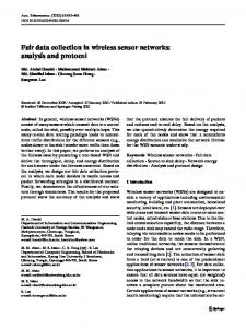
Fig. 1. Comparison of the Frantic and the Smart adversary; network strategy is KM. (S) stands for simulated results. Our claim then follows Equation 3: Pf (v)

= P r[Xv = 1] = P1 · P2v−1 · P3v−1

We observe that, to achieve Cr ∩ Cr−1 = ∅, ADV can randomly select two disjoint sets C1 and C2 and alternate between them. In other words, there is no need for ADV to move around the entire network. Since the probability of any sensor being chosen as a recipient is uniform, this type of ADV – which we refer to as Smart – has exactly the same probability of finding x as the Frantic ADV. We also note that, since the UWSN might be deployed over a wide geographical area, compromising some sensors might require more effort than others. Therefore, the Smart ADV can restrict its activity to the most accessible (easiest to compromise) sensors C1 ∪ C2 and thus minimize physical mobility. Figure 1 shows that survival probability at each round is the same for both Frantic and Smart ADV-s. 3.4

At any subsequent round, the chain will move to: • Sc , if ADV finds the target value • Sr , if ADV does not compromise the sensor storing the target value and no currently compromised sensor receives it. The number of rounds the target value survives is the number of transactions for the chain to reach Sc . From the analysis in Section 3.3, we build the transition matrix M of the Markov chain for the KM strategy, where each element mij represents the probability that the chain moves from state Si to state Sj :     m00 m0r m0c 0 P1 1 − P1 M =  mr0 mrr mrc  =  0 P2 · P3 1 − P2 · P3  mc0 mcr mcc 0 0 1 Note that Sc is an absorbing state (mcc = 1) and that S0 is a transient state, since the system cannot return to it (mi0 = 0, ∀i). Since the Markov chain is absorbing, the average absorbing time represents the expected ADV’s winning round. To easily compute the average absorbing time of the chain [15], we evaluate its fundamental matrix where each entry gives the expected number of times that the process is in a non-absorbing state. Based on M , the fundamental matrix is:   1 −P1 N= 0 1 − P2 · P3 Combining the fundamental matrix with the fact that the chain always starts from state S0 , we obtain the ADV’s expected winning round with the KM strategy:

MO vs KM: Expected Winning Round

We now show that ADV’s expected winning round is the same for both MO and KM defense strategies. We model the system by a Markov Chain with the following states: • S0 : represents the network at round 0, when ADV has not yet chosen any sensors to compromise. This is also the only initial state of the chain. • Sr : represents the network at round r > 0, when ADV corrupted a set of sensors Cr and is still looking for the target value, meaning that x was stored elsewhere and, after message exchange, no sensor in Cr received it. • Sc : represents the network at round r > 0, when ADV corrupted Cr and has found the target value. The system starts in state S0 and leaves it at round 1. It then reaches state Sr if sˇ1 ∈ / C1 and ˚ s1 ∈ / C1 ; otherwise, it moves to Sc and the game ends.

Exp = 1 +

P1 1 − P2 · P 3

(7)

For the MO strategy, it is trivial to see that the expected n winning round is 2k . Table 3 shows ADV’s expected winning round according to the previous analysis. It is clear that, on the average, both strategy provide the same survival rate of the target data. 3.5

Communication and Storage Costs

As shown in Table 4, MO and KM strategies introduce both storage and communication costs. As expected, communication overhead is higher for the latter. As far as storage overhead (determined by the number of messages a sensor receives in a single round), Table 4 shows the probability bounds that limit the queue sizes.

IEEE TRANSACTIONS ON NETWORKING SPECIAL ISSUE ON AUTONOMIC NETWORK COMPUTING

strategy MO KM

msg per round (r) n vn

msg tot v·n (r2 /2)n

7

stored data

received messages

√

P r[∃ si | Lri ≥ r + nr] ≤ e−r/2+ln n P r[∃ si | Lri ≥ 2er] ≤ 2−r+ln n

O(ln n) P r[∃ si | Mir ≥ 2er] ≤ 2−r+ln n

TABLE 4 Overhead comparison

1 SETTINGS: n = 100, k = 5 Move Once (A) Move Once (S) Keep Moving (A) Keep Moving (S) 0.8

survival probability

The bounds show that proposed defense strategies are viable. As for the maximum number of messages that could be sent to a single sensor, since each sensor selects its recipient peer uniformly and at random, this problem has a natural correspondence with the balls-and-bins model. We leverage the fact that when throwing n balls uniformly at random over n bins, the maximum load of a bin is O(log n) with probability at most 1/n [16]. That is, for the MO strategy, the maximum number of messages sent to a single sensor in one round is O(log n). We also provide a bound for the probability that the number of data items stored at a sensor do not exceed a certain value `. Let Lri be a random variable representing the number of data items stored by sensor si at round r. Clearly, E[Lri ] = r. Applying the method of bounded differences (a special case√of Azuma’s inequality) [16], we have that, for ` > r + rn:

0.6

0.4

0.2

0 0

10

20

30

40

50

round

Fig. 2. Survival rate for different defense strategies against Search-and-Erase. (S) and (A) stand for simulated and analytical results, respectively.

P r[Lr1 ≥ ` ∪ . . . ∪ Lrn ≥ `] ≤ nP r[Lr1 ≥ `] ≤ e−r/2+ln n As for the KM strategy, using the same notation, we still have that: P r[Lr1 ≥ ` ∪ . . . ∪ Lrn ≥ `] ≤ nP r[Lr1 ≥ `] However, with KM, the random variables: L11 , . . . , Lr1 are independent; hence, we can apply the Chernoff bound [16], obtaining (E[Lr1 ] = r): P r[Lr1 ≥ `] ≤ 2−r for ` > 2er. Therefore: P r[Lr1 ≥ ` ∪ . . . ∪ Lrn ≥ `] ≤ nP r[Lr1 ≥ `] ≤ 2−r+log2 n If we define the random variable Mir (which represents the number of messages received by si at round r), then with the same technique used above, we have: P r[M1r ≥ ` ∪ . . . ∪ Mnr ≥ `] ≤ nP r[M1r ≥ `] ≤ 2−r+log2 n 3.6

Summary

The above analysis makes it clear that the choice between MO and KM depends on the frequency of sink visits. Figure 2 shows target data survival probability against Search-and-Erase, given MO and KM defense strategies. With the former, ADV is guaranteed to win in at most n k rounds, whereas, with KM, target data survives somewhat longer. Nevertheless, for the first nk , MO performs better than KM. This is because the latter changes the location of target data at each round and, as discussed earlier, it affords ADV two chances to capture x in each round. Moreover, KM is obviously more expensive than the MO.

We conclude that, if v < nk , MO is the most effective and efficient strategy against Search-and-Erase.

4

E RASER

Recall that Eraser is not focused on any particular data. Its main goal is to delete as much data as possible before the next sink visit. As in section 3, we assume that ADV starts compromising sensors at round 1 and has v rounds at its disposal. We investigate the effectiveness of data dissemination strategies of Section 2.3 and estimate the amount of data surviving in network at each round. 4.1

DN

To maximize its advantage, ADV needs to always compromise the set of k sensors with the highest number of stored data items. It is easy to see that this is best achieved by moving in a round-robin fashion for the first n k rounds. In doing so, ADV deletes (r + 1) · k messages during the first r ≤ nk rounds. At round nk + 1, the k sensors that have the largest number of data items are those that have not been visited for the longest time, i.e., those compromised at round 1. Each of those sensors has by now accumulated nk values so that ADV can delete n values, total. Using the same argument for subsequent rounds, ADV needs to move in a round-robin fashion at any round r > nk and to delete n values per round. As n new measurements are introduced at every round, after round nk the number of values in the network remains

IEEE TRANSACTIONS ON NETWORKING SPECIAL ISSUE ON AUTONOMIC NETWORK COMPUTING

1000

stable. Thus, the number of remaining data items at round r is: DDN (r) = n

n

min r, k n no X )+ (n − i · k) DDN (r) =n − k · (min r, k i=1

otherwise. 4.2

900

average number of survived data in the network

if r = 0, while:

8

800

700

600

500

400

300 SETTINGS: n = 100, k = 5 Do Nothing (S) Do Nothing (A) Move Once (S) Move Once (A) Keep Moving (S) Keep Moving (A)

MO 200

Using an argument similar to that in Section 4.1, with the MO strategy, ADV needs to move in a round-robin fashion to assure that, at any round, it compromises the set of sensors with the largest number of data items. Let pM O (r) be the probability that a given data item survives r rounds: n  min {r−1,   Y k −1}  k k 1− (8) pM O (r) = 1 − n n − ik i=0 The component on the left is the probability that the data was sent to a non-compromised sensor. The factor with i = 0 represents the probability that the data has been acquired by a non-compromised sensor. The factors with i ≥ 1 account for the probability that ADV did not compromise the sensor holding the value, i rounds after it has been sensed. The product has at most nk factors because the value migrates just once and ADV is guaranteed to delete it by round nk . Thus the average number of values remaining at round r is: ( n if r = 0 Pr pM O (r) DM O (r) = n · 1− k + i=1 (n · pM O (i)) otherwise ( n) (9) 4.3

KM

With the KM strategy, at each round, each sensor offloads all of its stored data to randomly chosen peers. Thus, ADV is no longer sure that the least recently visited sensors are the ones holding the largest number of data items. In this scenario, ADV does not need to move in a round-robin fashion. However, it is still in its interest to choose Cr such that Cr ∩ Cr−1 = ∅. Let pKM (r) be the probability that a particular value survives r rounds: 2    r−1  k k k 1− · 1− pKM (r) = 1 − n n−k n (10) The squared factor is the probability that a value is sensed by, and sent to, some non-compromised sensor. The factor exponentiated to the power of r − 1 accounts for the probability that ADV did not compromise the sensor holding that value, nor any of the comprised sensors received it, during subsequent r − 1 rounds.

100 0

10

20

30

40

50

round

Fig. 3. Survival rate of different defense strategies against Eraser. (S) and (A) stand for simulated and analytical results, respectively.

To estimate the number of data items surviving Eraser at round r, we need to take into account data sensed at any round 0 ≤ i ≤ r, and the probability that they survived until the current round. The number of data items in the network at round r is:  n if r = 0 Pr DKM (r) = n · pKM (r) + i=1 (n · pKM (r)) otherwise (11) 4.4

Summary

It might seem surprising that the most effective strategy against an Eraser is DN. Figure 3 shows that data survival is maximized if acquired data is kept in situ. Indeed, if data does not migrate, ADV can only erase items found in the storage of compromised sensors. If data is moved around the network, either once or at any round, ADV can delete items found in compromised sensors, as well as items that those sensors receive from their non-compromised counterparts. In the same figure, the number of remaining data items with the DN and MO strategies, exhibit a sudden drop of k messages at round nk . This is because ADV starts compromising sensors at round 1, while sensing starts at round 0. Nevertheless, by round nk , ADV deletes all data sensed at round 0, and this one-round advantage is lost.

5

R EPLICATION

In this section we investigate the effects of data replication. Along with data migration, data replication is a natural and intuitive technique for increasing the odds of data survival. If we assume that each data item is replicated R times and each replica is treated independently, the end-result is an R-fold increase in storage and communication costs. In this paper we assume all data is

IEEE TRANSACTIONS ON NETWORKING SPECIAL ISSUE ON AUTONOMIC NETWORK COMPUTING

treated equally within the network; however, in case sensors are aware of the relevance of the sensed data, they might replicate data according to some prioritization policy. For example, in a fire-prevention monitoring sensor network, sensors might only replicate measurements that are above a critical threshold. This way, the overhead incurred in data storage and communication would be sensibly decreased. In the following we show the gain in data survival that can be achieved with replication. 5.1

Survival probability 1 0.9 0.8 0.7 0.6 0.5 0.4 0.3 0.2 0.1 0

0

Search-and-Erase

2

4

6

Rounds

In order to succeed, a Search-and-Erase must delete all R copies of target data. Let Xi,j = 1 denote the event of i-th replica surviving up to round j, and Xi,j = 0 denote the event of ADV erasing it by round j. The probability PRv of no replicas surviving up to round v is:

9

8 10 12 14 16 18 20 1

2

3

4

5

Replicas

Fig. 4. Survival of Replicated Data against Search-andErase using the Frantic strategy; network strategy is KM.

PRv = P r[X1,v = 0 ∧ . . . ∧ XR,v = 0] = P r[X1,v = 0]R Then, the probability of at least one replica surviving to round v is: PRv = 1 − PRv (12) With the MO strategy, using the results from Seck tion 3.2, we have that P r[Xi,j = 1] = n−jk . Plugging this into Equation 12 yields: !R v−1 Y k PRv = 1 − 1 − 1− (13) n − ik i=0 With the KM strategy, according to Equation 2: P r[Xi,j = 1] = P1 · P2j−1 · P3j−1 Using the probability in Equation 12: PRv = 1 − PRv = 1 − (1 − P1 · P2v−1 · P3v−1 )R

(14)

Figure 4 shows how data survival rate increases with replication. With no replication (R = 1) data survives 20 rounds with probability 0.122; at the same round, if R = 5, probability of at least one copy surviving is 0.48.

5.2

Eraser

Since Eraser deletes all data it encounters, replication naturally increases survival rate for data items acquired by any sensor at any round. Effectiveness of replication is estimated by the number of distinct data items that survive up to round v (replicas of the same data are not taken into account). 5.2.1

MO strategy

With the MO strategy, the probability of all R replicas of a given data item being erased by round r is (1−pM O (r))R . Thus, the probability of at least one replica surviving at round r is 1 − (1 − pM O (r))R .

Using an argument similar to that in Section 3.3, we can derive the overall number of distinct data items that survive by round r:  n if r = 0 R P DM O (r) = r R n · (1 − (1 − p (i)) ) otherwise M O i=0 (15) 5.2.2 KM strategy With R-fold replication, the probability of at least one replica surviving r rounds is: 1 − (1 − pKM (r))R . Here we also use the argument of Section 3.3 to estimate the overall number of distinct data items surviving by round r:  if r = 0   n R R DKM (r)= n(1P − (1 − pKM (r)) )+   r + i=1 n · (1 − (1 − pKM (i))R ) otherwise (16) Figure 5 shows how data migration and replication together affect data survival against Eraser. As shown in Section 4, without replication, DN is the best strategy against this kind of adversary. However, data migration improves data survival even with a single replica (i.e., R = 2). Figure 6 shows how replication coupled with the KM strategy improves data survival. After 20 rounds, without replication, ADV erases 80% of all data, whereas, with R = 5, ADV deletes only 15%. This clearly represents a dramatic increase in data survival and confirms that KM is the best strategy when used with replication.

6

R ELATED W ORK

Wireless Sensor Networks and Mobile Ad Hoc Networks have so many similarities that very often results of the one can be applied to the other. Even if researchers are mainly engaged to devise efficient routing or almost optimal clustering protocols, many results are also proposed for MANET data availability: those network

IEEE TRANSACTIONS ON NETWORKING SPECIAL ISSUE ON AUTONOMIC NETWORK COMPUTING

1400

average number of survived data in the network

1200

1000

800

600

400

SETTINGS: n = 100, k = 5 Do Nothing (A) Move Once (A) Keep Moving (A) Move Once with R=2 (A) Keep Moving with R=2 (A)

200

0 0

5

10

15

20

25

30

round

Fig. 5. Average number of data items surviving Eraser, with and without replication. (A) stands for analytical results.

Average number of survived data in the network

1800 1600 1400 1200 1000 800 600 400 200 0 20 15 10 5 5

4 Replicas

3

2

181920 151617 121314 9 1011 Rounds 6 7 8 3 4 5 2 1 1 0

Fig. 6. Effects of replication against Eraser using the Frantic strategy; network strategy is KM.

face challenges such as communication faults, network partitions or malicious node behaviors. In those contexts, a research thread aims to buttress data availability to any MANET node, even in case of network fragmentation or congestion. Hara et al. [17] introduced some simple and effective replication algorithms, such that even if a node lies in a disconnected partition, it can still access any data with high probability. A mechanism to provide replica consistency in case of updates to the original data and simple location management technique to guarantee that nodes access the closest replica are also presented in their work. Data replication effectiveness in partitioned MANETs is also addressed by Giannuzzi et al. in [14]. The authors show how data access in the network is highly related to the number of replicas as well as to the network density and to the nodes’ transmission radius. Chessa et al. [3] introduced a distributed data storage approach for mobile wireless networks, based on the

10

peer-to-peer paradigm. Their technique provides support to create and share files under a write-once model, and also ensures data confidentiality and dependability by encoding files in a Redundant Residue Number System (RRNS). Benenson et al. [29] investigated possible strategies for preventing a mobile adversary from learning certain sensed data and/or for preventing contiguous unauthorized access, once the data has been learned. Data is randomly moved around the network and an adversary who once had access to the data stored at some captured sensor, must compromise other sensors in order to retain its access to the target data. Several algorithms are introduced to provide efficient data retrieval and update. The authors of [1], [25], [4] statistically improve data confidentiality and data availability in hostile MANET environments, where both insider and outsider adversaries may be present, by leveraging the existence of multiple paths between end-nodes. A more recent result addressing data availability in WSNs is [18]. It develops a scheme to maximize the amount of data recovered at the sink and shows how the proposed scheme improves data availability when a portion of the network is invalidated by natural disasters, such as floods or earthquakes. Our work is inspired by a seminal paper for UWSNs [8]. The authors introduce an adversarial model with limited scope and show how data survival can be achieved with non-cryptographic techniques. The use of cryptography in UWSNs was recently addressed either to protect data confidentiality in [9] or to achieve data authentication, as in [10]. Collaborative approaches in UWSNs to cope with the mobile adversary can be found also in [23] and [7]. A broader analysis of the different mobile adversary’s goals can be found in [21]. UWSNs have also recently been considered in the context of minimizing storage and bandwidth overhead due to data authentication in the presence of a powerful adversary [22]. The proposed forward-secure aggregate authentication techniques can efficiently provide forward security, i.e., having compromised a sensor, the adversary is unable to modify any data collected prior to compromise.

7

C ONCLUSIONS

In this paper, we introduced a new mobile adversary model specific to unattended WSNs operating in hostile settings. We introduced some simple non-cryptographic strategies for maximizing data survival in the presence of an adversary that has been characterized in different flavors, based on its goals. A thorough analysis completely frames the quality of the devised strategies, when applied to the different adversary models. Data dissemination and replication strategies described here demonstrate significantly improved probability of data survival. Finally, extensive simulations support our analytical findings.

IEEE TRANSACTIONS ON NETWORKING SPECIAL ISSUE ON AUTONOMIC NETWORK COMPUTING

The use of cryptography in the described framework is currently being explored.

8

ACKNOWLEDGMENTS

The authors are grateful to the anonymous referees for their insightful and useful comments on the earlier version of this paper. This research was supported in part by: • The Spanish Ministry of Science and Education through projects TSI2007-65406-C03-01 “E-AEGIS” and CONSOLIDER CSD2007- 00004 “ARES”, and by the Government of Catalonia under grant 2005 SGR 00446. • The EU FP6 projects: “European Satellite Communications Network of Excellence” (SatNEx II, IST27393); PERSONA (contract N. 045459); INTERMEDIA (contract N.38419). • An award from the US Army Research Office (ARO) contract W911NF0410280 as well as a grant from the US Fulbright Foundation.

R EFERENCES [1]

V. Berman and B. Mukherjee. Data security in manets using multipath routing and directional transmission. In IEEE International Conference on Communications (ICC’06), pages 2322–2328, 2006. [2] A. Caruso, A. Urpi, S. Chessa, and S. De. Gps-free coordinate assignment and routing in wireless sensor networks. In 24th Joint Conference of the IEEE Computer and Communications Societies (INFOCOM ’05), pages 150–160, 2005. [3] S. Chessa and P. Maestrini. Dependable and secure data storage and retrieval in mobile, wireless networks. In International Conference on Dependable Systems and Networks (DSN ’03), pages 207–216, 2003. [4] M. Conti, R. Di Pietro, and L. V. Mancini. ECCE: Enhanced cooperative channel establishment for secure pair-wise communication in wireless sensor networks. Ad Hoc Networks (Elsevier), 5(1):49– 62, 2007. [5] B. Deb, S. Bhatnagar, and B. Nath. Reinform: Reliable information forwarding using multiple paths in sensor networks. In 28th IEEE International Conference on Local Computer Networks (LCN ’03), pages 406–415, 2003. [6] J. Deng, C. Hartung, R. Han, and S. Mishra. A Practical Study of Transitory Master Key Establishment ForWireless Sensor Networks. 1st International Conference on Security and Privacy for Emerging Areas in Communications Networks (SecureComm ’05), pages 289–302, 2005. [7] R. Di Pietro, D. Ma, G. Tsudik, and C. Soriente. POSH: Proactive co-operative self-healing in unattended sensor networks. In 27th IEEE International Symposium on Reliable Distributed Systems (SRDS’ 08), pages 185–194, 2008. [8] R. Di Pietro, L. V. Mancini, C. Soriente, A. Spognardi, and G. Tsudik. Catch me (if you can): Data survival in unattended sensor networks. In Sixth Annual IEEE International Conference on Pervasive Computing and Communications, 2008 (PerCom’08)., pages 185–194, New York, NY, USA, 2008. IEEE press. [9] R. Di Pietro, L.V. Mancini, C. Soriente, A. Spognardi, and G. Tsudik. Playing hide-and-seek with a focused mobile adversary in unattended sensor networks. Ad Hoc Networks (Elsevier). Special Issue on Privacy and Security in Wireless Sensor and Ad Hoc Networks, 2009. [10] R. Di Pietro, C. Soriente, A. Spognardi, and G. Tsudik. Collaborative authentication in unattended wsns. In ACM Conference on Wireless Network Security (ACM WiSec ’09), 2009. [11] Y. Frankel, P. Gemmell, P. D. MacKenzie, and M. Yung. Proactive RSA. In 17th Annual International Cryptology Conference on Advances in Cryptology (CRYPTO ’97), pages 440–454, 1997.

11

[12] S. Ganeriwal, R. Kumar, and M. B. Srivastava. Timing-sync protocol for sensor networks. In 1st international conference on Embedded networked sensor systems (SenSys ’03), pages 138–149, 2003. [13] D. Ganesan, R. Govindan, S. Shenker, and D. Estrin. Highlyresilient, energy-efficient multipath routing in wireless sensor networks. SIGMOBILE Mobile Computing and Communications Review, 5(4):11–25, 2001. [14] V. Gianuzzi. Data replication effectiveness in mobile ad-hoc networks. In ACM Workshop on Performance Evaluation of Wireless Ad Hoc,Sensor, and Ubiquitous Networks (PE-WASUN ’04), pages 17–22, 2004. [15] C. M. Grinstead and J. L. Snell. Introduction to probability. Random House, second edition, 2003. 410 pp. [16] M. Habib, C. McDiarmid, J. Ramirez-Alfonsin, and B. Reed. Probabilistic Methods for Algorithmic Discrete Mathematics. SpringerVerlag, 1998. [17] T. Hara and S. K. Madria. Data replication for improving data accessibility in ad hoc networks. IEEE Trans. Mob. Comput., 5(11):1515–1532, 2006. [18] A. Kamra, V. Misra, J. Feldman, and D. Rubenstein. Growth codes: maximizing sensor network data persistence. SIGCOMM Comput. Commun. Rev., 36(4):255–266, 2006. [19] C. Karlof and D. Wagner. Secure routing in wireless sensor networks: attacks and countermeasures. Ad Hoc Networks, 1(23):293–315, 2003. [20] B. Karp and H. T. Kung. GPSR: Greedy perimeter stateless routing for wireless networks. In 6th ACM/IEEE International Conference on Mobile Computing and Networking (MobiCom ’00), pages 243–254, 2000. [21] D. Ma, C. Soriente, and G. Tsudik. New adversary and new threats: Security in unattended sensor networks. IEEE Network, 6(2), 2009. [22] D. Ma and G. Tsudik. Extended abstract: Forward-secure sequential aggregate authentication. In 2007 IEEE Symposium on Security and Privacy (SP ’07), pages 86–91, 2007. [23] D. Ma and G. Tsudik. DISH: Distributed self-healing in unattended sensor networks. In 10th International Symposium on Stabilization, Safety, and Security of Distributed Systems (SSS’ 08), 2008. [24] R. Ostrovsky and M. Yung. How to withstand mobile virus attacks. In 10th ACM Symposium on Princiles of Distributed Computing (PODC ’91), pages 51–59, 1991. [25] P. Papadimitratos and Z.J. Haas. Secure data communication in mobile ad hoc networks. IEEE JSAC, 24(2):343–356, 2006. [26] M. O. Rabin. Efficient dispersal of information for security, load balancing, and fault tolerance. J. ACM, 36(2):335–348, 1989. [27] T. Rabin. A simplified approach to threshold and proactive RSA. In 18th Annual International Cryptology Conference on Advances in Cryptology (CRYPTO ’98), pages 89–104, 1998. [28] A. Shamir. How to share a secret. Commun. ACM, 22(11):612–613, 1979. [29] P.M. Cholewinski Z. Benenson and F.C. Freiling. Simple evasive data storage in sensor networks. In International Conference on Parallel and Distributed Computing Systems (PDCS ’05), pages 779– 784, 2005.

A PPENDIX E RASURE C ODES As demonstrated earlier, replication is effective against Search-and-Erase and Eraser. However, replication results in a commensurate increase in storage and bandwidth costs. One alternative is to use well-known erasure codes in order to improve data survival probability. To this end, in the rest of this section we compare erasure codes against plain replication assuming the KM defense strategy. We adopt IDA (Information Dispersal Algorithm) [26] as the underlying erasure code, mainly because of its optimal bandwidth usage. Using IDA, it is possible to break an information in an arbitrary number of fragments,

IEEE TRANSACTIONS ON NETWORKING SPECIAL ISSUE ON AUTONOMIC NETWORK COMPUTING

1

Search-and-Erase

SETTINGS: n = 100, k = 5 Replication 5 (A) Erasure-Code 2/6 (A) Erasure-Code 4/6 (A)

0.8

A Search-and-Erase needs to delete at least f 00 + 1 fragments of target data in order to succeed. The probability that ADV deletes one fragment by round r is: 1−pKM (r) If each data item is split into f 0 + f 00 fragments, the probability that the value is irrecoverable is the same as the probability of at least f 00 + 1 fragments being deleted by round r:

1

survival probability

0.98 0.96

0.6

0.94 0.92 0.4 0.9 0

1

2

3

4

5

6

7

p¯(r) = 0.2

0 fX +f 00

i=f 00 +1

0 0

10

20

30

40

12

50



   0 00 f 0 + f 00 i (1 − pKM (r)) pKM (r)f +f −i i

Thus, the probability of at least f 0 fragments surviving by round r is: p(r) = 1 − p¯(r).

round

Fig. 7. Replication vs erasure codes. (A) stands analytical results. such that reconstructing the original information would only require a subset of the original fragments. Dispersal and reconstruction are computationally efficient, while a careful choice of the parameters can make dispersal also space efficient. The basic idea is to split each data item into F = f 0 +f 00 fragments and treat them independently, off-loading each of them to a random recipient. As long as f 0 out of F fragments survive, the sink can reconstruct the original value. Indeed, f 00 characterizes the IDA reliability. According to [26], a value is considered as a sequence of characters b1 , ..., bN . Let p be the smallest prime such that bi < p. Then, each fragment is composed of fN0 elements of Zp . Thus, the number of bits to represent a value after fragmentation is: (f 0 + f 00 ) · fN0 · log(p). For a fair comparison, we need to use the number of bits for fragmentation and replication, i.e.: R · |x| = (f 0 + f 00 )

N · log(p) f0

Comparison with Replication We now compare fragmentation with plain replication. We assume that each data item is one byte. With replication and R = 5, the total number of bits is 40. With fragmentation, using the same number of bits, we consider two cases: (1) f 0 = 2, f 00 = 6, and (2) f 0 = 4, f 00 = 6. As shown in Figure 7, replication works better than fragmentation, except for the first few rounds. Indeed, up to r = 5, fragmentation performs (slightly) better than replication. This can be explained focusing on the first round: ADV can only win by deleting at least f 00 +1 fragments. Whereas, in case of replication, it has to delete exactly r items. However, the number of fragments is higher than the number of replicas. Therefore, as rounds go by, fragments are deleted with greater probability. As the number of fragments decreases, fragmentation starts loosing its appeal. We note that, with replication, as long as just one replica survives, ADV looses, while with fragmentation, at least f 0 fragments must survive. Figure 7 shows that the advantage of fragmentation over replication vanishes after round 5. We conclude that fragmentation does not seem worthwhile.