Data, syntax and semantics (pdf) - Department of Computer Science

Data, Syntax and Semantics An Introduction to Modelling Programming Languages

J V Tucker Department of Computer Science University of Wales Swansea Singleton Park Swansea SA2 8PP Wales

K Stephenson QinetiQ St Andrews Road Malvern WR14 3PS England

c Copyright J V Tucker and K Stephenson °2006 This is an almost complete first draft of a text-book. It is the text for a second year undergraduate course on the Theory of Programming Languages at Swansea. Criticisms and suggestions are most welcome.

20th March 2006

“. . . yet muste you and all men take heed, that . . . in al mennes workes, you be not abused by their autoritye, but evermore attend to their reasons, and examine them well, ever regarding more what is saide, and how it is proved, then who saieth it: for autoritie often times deceaveth many menne.” Robert Recorde The Castle of Knowledge, 1556

Contents 1 Introduction 1.1 Science and the aims of modelling programming languages . . . 1.2 Some Scientific Questions about Programming Languages . . . . 1.3 A Simple Imperative Programming Language and its Extensions 1.3.1 What is a while Program? . . . . . . . . . . . . . . . . . 1.3.2 Core Constructs . . . . . . . . . . . . . . . . . . . . . . . 1.4 Where do we find while programs? . . . . . . . . . . . . . . . . 1.4.1 Gallery of Imperative Languages . . . . . . . . . . . . . 1.4.2 Pseudocode and Algorithms . . . . . . . . . . . . . . . . 1.4.3 Object-Oriented Languages . . . . . . . . . . . . . . . . 1.4.4 Algebraic, Functional and Logic Languages . . . . . . . . 1.5 Additional Constructs of Interest . . . . . . . . . . . . . . . . . 1.5.1 Data . . . . . . . . . . . . . . . . . . . . . . . . . . . . . 1.5.2 Importing Data Types . . . . . . . . . . . . . . . . . . . 1.5.3 Input and Output . . . . . . . . . . . . . . . . . . . . . . 1.5.4 Atomic Statements . . . . . . . . . . . . . . . . . . . . . 1.5.5 Control Constructs . . . . . . . . . . . . . . . . . . . . . 1.5.6 Exception and Error handling . . . . . . . . . . . . . . . 1.5.7 Non-determinism . . . . . . . . . . . . . . . . . . . . . . 1.5.8 Procedures, Functions, Modules and Program Structure . 1.6 Conclusion . . . . . . . . . . . . . . . . . . . . . . . . . . . . . . 1.6.1 Kernel and Extensions . . . . . . . . . . . . . . . . . . . 2 Origins of Programming Languages 2.1 Historical Pitfalls . . . . . . . . . . . . . . . . . . . . . . 2.2 The Analytical Engine and its Programming . . . . . . . 2.3 Development of Universal Machines . . . . . . . . . . . . 2.4 Early Programming in the Decade 1945-1954 . . . . . . . 2.5 The Development of High Level Programming Languages 2.5.1 Early Tools . . . . . . . . . . . . . . . . . . . . . 2.5.2 Languages . . . . . . . . . . . . . . . . . . . . . . 2.5.3 Syntax . . . . . . . . . . . . . . . . . . . . . . . . 2.5.4 Declarative languages . . . . . . . . . . . . . . . . 2.5.5 Applications . . . . . . . . . . . . . . . . . . . . . 2.6 Specification and Correctness . . . . . . . . . . . . . . . 2.7 Data Types and Modularity . . . . . . . . . . . . . . . . i

. . . . . . . . . . . .

. . . . . . . . . . . .

. . . . . . . . . . . .

. . . . . . . . . . . .

. . . . . . . . . . . . . . . . . . . . . . . . . . . . . . . . .

. . . . . . . . . . . . . . . . . . . . . . . . . . . . . . . . .

. . . . . . . . . . . . . . . . . . . . . . . . . . . . . . . . .

. . . . . . . . . . . . . . . . . . . . . . . . . . . . . . . . .

. . . . . . . . . . . . . . . . . . . . . . . . . . . . . . . . .

. . . . . . . . . . . . . . . . . . . . . . . . . . . . . . . . .

. . . . . . . . . . . . . . . . . . . . . . . . . . . . . . . . .

. . . . . . . . . . . . . . . . . . . . . . . . . . . . . . . . .

. . . . . . . . . . . . . . . . . . . . .

1 2 3 6 7 10 12 13 15 15 17 18 18 20 20 20 21 22 22 23 24 24

. . . . . . . . . . . .

29 30 30 34 36 39 39 40 42 44 45 46 47

ii

I

CONTENTS

Data

3 Basic Data Types and Algebras 3.1 What is an Algebra? . . . . . . . . . . . 3.2 Algebras of Booleans . . . . . . . . . . . 3.2.1 Standard Booleans . . . . . . . . 3.2.2 Bits . . . . . . . . . . . . . . . . 3.2.3 Equivalence of Booleans and Bits 3.2.4 Three-Valued Booleans . . . . . . 3.3 Algebras of Natural Numbers . . . . . . 3.3.1 Basic Arithmetic . . . . . . . . . 3.3.2 Tests . . . . . . . . . . . . . . . . 3.3.3 Decimal versus Binary . . . . . . 3.3.4 Partial Functions . . . . . . . . . 3.4 Algebras of Integers and Rationals . . . 3.4.1 Algebras of Integer Numbers . . . 3.4.2 Algebras of Rationals . . . . . . . 3.5 Algebras of Real Numbers . . . . . . . . 3.5.1 Measurements and Real Numbers 3.5.2 Algebras of Real Numbers . . . . 3.6 Data and the Analytical Engine . . . . . 3.7 Algebras of Strings . . . . . . . . . . . . 3.7.1 Constructing Strings . . . . . . . 3.7.2 Manipulating Strings . . . . . . .

49 . . . . . . . . . . . . . . . . . . . . .

. . . . . . . . . . . . . . . . . . . . .

. . . . . . . . . . . . . . . . . . . . .

. . . . . . . . . . . . . . . . . . . . .

. . . . . . . . . . . . . . . . . . . . .

. . . . . . . . . . . . . . . . . . . . .

. . . . . . . . . . . . . . . . . . . . .

. . . . . . . . . . . . . . . . . . . . .

. . . . . . . . . . . . . . . . . . . . .

. . . . . . . . . . . . . . . . . . . . .

. . . . . . . . . . . . . . . . . . . . .

. . . . . . . . . . . . . . . . . . . . .

53 54 57 57 58 59 60 62 62 64 66 67 67 68 68 70 70 71 73 74 75 75

4 Interfaces and Signatures, Implementations and Algebras 4.1 Formal Definition of a Signature . . . . . . . . . . . . . . . . 4.1.1 An Example of a Signature . . . . . . . . . . . . . . 4.1.2 General Definition of a Signature . . . . . . . . . . . 4.2 Examples of Signatures . . . . . . . . . . . . . . . . . . . . . 4.2.1 Examples of Signatures for Basic Data Types . . . . 4.2.2 Signature for Subsets . . . . . . . . . . . . . . . . . . 4.2.3 Signature for Strings . . . . . . . . . . . . . . . . . . 4.2.4 Storage Media . . . . . . . . . . . . . . . . . . . . . . 4.2.5 Machines . . . . . . . . . . . . . . . . . . . . . . . . 4.3 Formal Definition of an Algebra . . . . . . . . . . . . . . . . 4.3.1 General Notation and Examples . . . . . . . . . . . . 4.4 Examples of Algebras . . . . . . . . . . . . . . . . . . . . . . 4.4.1 Examples of Algebras for Basic Data Types . . . . . 4.4.2 Storage Media . . . . . . . . . . . . . . . . . . . . . . 4.4.3 Machines . . . . . . . . . . . . . . . . . . . . . . . . 4.4.4 Sets . . . . . . . . . . . . . . . . . . . . . . . . . . . 4.4.5 Strings . . . . . . . . . . . . . . . . . . . . . . . . . . 4.5 Algebras with Booleans and Flags . . . . . . . . . . . . . . . 4.5.1 Algebras with Booleans . . . . . . . . . . . . . . . . . 4.5.2 Algebras with an Unspecified Element . . . . . . . .

. . . . . . . . . . . . . . . . . . . .

. . . . . . . . . . . . . . . . . . . .

. . . . . . . . . . . . . . . . . . . .

. . . . . . . . . . . . . . . . . . . .

. . . . . . . . . . . . . . . . . . . .

. . . . . . . . . . . . . . . . . . . .

. . . . . . . . . . . . . . . . . . . .

. . . . . . . . . . . . . . . . . . . .

. . . . . . . . . . . . . . . . . . . .

. . . . . . . . . . . . . . . . . . . .

. . . . . . . . . . . . . . . . . . . .

83 85 85 86 89 89 91 92 93 93 94 95 96 96 98 99 99 100 101 101 103

. . . . . . . . . . . . . . . . . . . . .

. . . . . . . . . . . . . . . . . . . . .

. . . . . . . . . . . . . . . . . . . . .

. . . . . . . . . . . . . . . . . . . . .

. . . . . . . . . . . . . . . . . . . . .

. . . . . . . . . . . . . . . . . . . . .

. . . . . . . . . . . . . . . . . . . . .

. . . . . . . . . . . . . . . . . . . . .

. . . . . . . . . . . . . . . . . . . . .

. . . . . . . . . . . . . . . . . . . . .

iii

CONTENTS 4.6 4.7

4.8 4.9

Generators and Constructors . . . . . . . . Subalgebras . . . . . . . . . . . . . . . . . 4.7.1 Examples of Subalgebras . . . . . . 4.7.2 General Definition of Subalgebras . Expansions and Reducts . . . . . . . . . . Importing Algebras . . . . . . . . . . . . . 4.9.1 Importing the Booleans . . . . . . 4.9.2 Importing a Data Type in General 4.9.3 Example . . . . . . . . . . . . . . .

. . . . . . . . .

. . . . . . . . .

. . . . . . . . .

. . . . . . . . .

. . . . . . . . .

. . . . . . . . .

. . . . . . . . .

. . . . . . . . .

. . . . . . . . .

. . . . . . . . .

. . . . . . . . .

5 Specifications and Axioms 5.1 Classes of Algebras . . . . . . . . . . . . . . . . . . . . . . . . 5.1.1 One Signature, Many Algebras . . . . . . . . . . . . . 5.1.2 Reasoning and Verification . . . . . . . . . . . . . . . . 5.2 Classes of Algebras Modelling Implementations of the Integers 5.3 Axiomatic Specification of Commutative Rings . . . . . . . . . 5.3.1 The Specification . . . . . . . . . . . . . . . . . . . . . 5.3.2 Deducing Further Laws . . . . . . . . . . . . . . . . . . 5.3.3 Solving Quadratic Equations in a Commutative Ring . 5.4 Axiomatic Specification of Fields . . . . . . . . . . . . . . . . 5.5 Axiomatic Specification of Groups and Abelian Groups . . . . 5.5.1 The Specification . . . . . . . . . . . . . . . . . . . . . 5.5.2 Groups of Transformations . . . . . . . . . . . . . . . . 5.5.3 Matrix Transformations . . . . . . . . . . . . . . . . . 5.5.4 Reasoning with the Group Axioms . . . . . . . . . . . 5.6 Boolean Algebra . . . . . . . . . . . . . . . . . . . . . . . . . 5.7 Current Position . . . . . . . . . . . . . . . . . . . . . . . . .

. . . . . . . . . . . . . . . . . . . . . . . . .

. . . . . . . . . . . . . . . . . . . . . . . . .

. . . . . . . . . . . . . . . . . . . . . . . . .

. . . . . . . . . . . . . . . . . . . . . . . . .

. . . . . . . . . . . . . . . . . . . . . . . . .

. . . . . . . . . . . . . . . . . . . . . . . . .

. . . . . . . . . . . . . . . . . . . . . . . . .

6 Examples: Data Structures, Files, Streams and Spatial Objects 6.1 Records . . . . . . . . . . . . . . . . . . . . . . . . . . . . . . . . . . . . . 6.1.1 Signature/Interface of Records . . . . . . . . . . . . . . . . . . . . . 6.1.2 Algebra/Implementation of Records . . . . . . . . . . . . . . . . . . 6.2 Dynamic Arrays . . . . . . . . . . . . . . . . . . . . . . . . . . . . . . . . . 6.2.1 Signature/Interface of Dynamic Arrays . . . . . . . . . . . . . . . . 6.2.2 Algebra/Implementation of Dynamic Arrays . . . . . . . . . . . . . 6.3 Algebras of Files . . . . . . . . . . . . . . . . . . . . . . . . . . . . . . . . 6.3.1 A Simple Model of Files . . . . . . . . . . . . . . . . . . . . . . . . 6.4 Time and Data: A Data Type of Infinite Streams . . . . . . . . . . . . . . 6.4.1 What is a stream? . . . . . . . . . . . . . . . . . . . . . . . . . . . 6.4.2 Time . . . . . . . . . . . . . . . . . . . . . . . . . . . . . . . . . . . 6.4.3 Streams of Elements . . . . . . . . . . . . . . . . . . . . . . . . . . 6.4.4 Algebra/Implementation . . . . . . . . . . . . . . . . . . . . . . . . 6.4.5 Finitely Determined Stream Transformations and Stream Predicates 6.4.6 Decimal Representation of Real Numbers . . . . . . . . . . . . . . . 6.5 Space and Data: A Data Type of Spatial Objects . . . . . . . . . . . . . . 6.5.1 What is space? . . . . . . . . . . . . . . . . . . . . . . . . . . . . .

. . . . . . . . . . . . . . . . . . . . . . . . . . . . . . . . . . . . . . . . . .

. . . . . . . . .

. . . . . . . . .

105 108 109 110 112 114 115 118 120

. . . . . . . . . . . . . . . .

127 . 128 . 129 . 130 . 131 . 134 . 134 . 135 . 138 . 140 . 143 . 143 . 145 . 146 . 147 . 148 . 149

. . . . . . . . . . . . . . . . .

157 . 160 . 160 . 161 . 163 . 164 . 165 . 168 . 168 . 172 . 173 . 173 . 175 . 176 . 176 . 179 . 183 . 184

iv

CONTENTS 6.5.2 6.5.3 6.5.4

Spatial objects . . . . . . . . . . . . . . . . . . . . . . . . . . . . . . . . 187 Operations on Spatial Objects . . . . . . . . . . . . . . . . . . . . . . . . 189 Volume Graphics and Constructive Volume Geometry . . . . . . . . . . . 191

7 Abstract Data Types and Homomorphisms 7.1 Comparing Decimal and Binary Algebras of Natural Numbers . . . . . . 7.1.1 Data Translation . . . . . . . . . . . . . . . . . . . . . . . . . . . 7.1.2 Operation Correspondence . . . . . . . . . . . . . . . . . . . . . . 7.2 Translations between Algebras of Data and Homomorphisms . . . . . . . 7.2.1 Basic Concept . . . . . . . . . . . . . . . . . . . . . . . . . . . . . 7.2.2 Homomorphisms and Binary Operations . . . . . . . . . . . . . . 7.2.3 Homomorphisms and Number Systems . . . . . . . . . . . . . . . 7.2.4 Homomorphisms and Machines . . . . . . . . . . . . . . . . . . . 7.3 Equivalence of Algebras of Data: Isomorphisms and Abstract Data Types 7.3.1 Inverses, Surjections, Injections and Bijections . . . . . . . . . . . 7.3.2 Isomorphisms . . . . . . . . . . . . . . . . . . . . . . . . . . . . . 7.3.3 Abstract Data Types . . . . . . . . . . . . . . . . . . . . . . . . . 7.4 Induction on the Natural Numbers . . . . . . . . . . . . . . . . . . . . . 7.4.1 Induction for Sets and Predicates . . . . . . . . . . . . . . . . . . 7.4.2 Course of Values Induction and Other Principles . . . . . . . . . . 7.4.3 Defining Functions by Primitive Recursion . . . . . . . . . . . . . 7.5 Naturals as an Abstract Data Type . . . . . . . . . . . . . . . . . . . . . 7.6 Digital Data Types and Computable Data Types . . . . . . . . . . . . . 7.6.1 Representing an Algebra using Natural Numbers . . . . . . . . . . 7.6.2 Algebraic Definition of Digital Data Types . . . . . . . . . . . . . 7.6.3 Computable Algebras . . . . . . . . . . . . . . . . . . . . . . . . . 7.7 Properties of Homomorphisms . . . . . . . . . . . . . . . . . . . . . . . . 7.8 Congruences and Quotient Algebras . . . . . . . . . . . . . . . . . . . . . 7.8.1 Equivalence Relations and Congruences . . . . . . . . . . . . . . . 7.8.2 Quotient Algebras . . . . . . . . . . . . . . . . . . . . . . . . . . 7.9 Homomorphism Theorem . . . . . . . . . . . . . . . . . . . . . . . . . . .

. . . . . . . . . . . . . . . . . . . . . . . . . .

. . . . . . . . . . . . . . . . . . . . . . . . . .

. . . . . . . . . . . . . . . . . . . . . . . . . .

205 . 208 . 209 . 209 . 211 . 211 . 214 . 215 . 220 . 221 . 222 . 224 . 226 . 227 . 228 . 230 . 230 . 232 . 235 . 236 . 238 . 238 . 239 . 241 . 241 . 242 . 244

8 Terms and Equations 8.1 Terms . . . . . . . . . . . . . . . . . . . . . . . . . . . . . . 8.1.1 What is a Term? . . . . . . . . . . . . . . . . . . . . 8.1.2 Single-Sorted Terms . . . . . . . . . . . . . . . . . . 8.1.3 Many-Sorted Terms . . . . . . . . . . . . . . . . . . . 8.2 Induction on Terms . . . . . . . . . . . . . . . . . . . . . . . 8.2.1 Principle of Induction for Single-Sorted Terms . . . . 8.2.2 Principle of Induction for Many-Sorted Terms . . . . 8.2.3 Functions on Terms . . . . . . . . . . . . . . . . . . . 8.2.4 Comparing Induction on Natural Numbers and Terms 8.3 Terms and Trees . . . . . . . . . . . . . . . . . . . . . . . . 8.3.1 Examples of Trees for Terms . . . . . . . . . . . . . . 8.3.2 General Definitions by Structural Induction . . . . . 8.4 Term Evaluation . . . . . . . . . . . . . . . . . . . . . . . .

. . . . . . . . . . . . .

. . . . . . . . . . . . .

. . . . . . . . . . . . .

. . . . . . . . . . . . .

. . . . . . . . . . . . .

. . . . . . . . . . . . .

. . . . . . . . . . . . .

. . . . . . . . . . . . .

. . . . . . . . . . . . .

. . . . . . . . . . . . .

. . . . . . . . . . . . .

251 252 252 255 260 265 265 266 267 270 271 271 272 274

v

CONTENTS 8.5

8.6 8.7

Equations . . . . . . . . . . . . . . . . . . . . . . . . . . . . . . . . 8.5.1 What is an equation? . . . . . . . . . . . . . . . . . . . . . . 8.5.2 Equations, Satisfiability and Validity . . . . . . . . . . . . . 8.5.3 Equations are Preserved by Homomorphisms . . . . . . . . . Term Algebras . . . . . . . . . . . . . . . . . . . . . . . . . . . . . Homomorphisms and Terms . . . . . . . . . . . . . . . . . . . . . . 8.7.1 Structural Induction, Term Evaluation and Homomorphisms 8.7.2 Initiality . . . . . . . . . . . . . . . . . . . . . . . . . . . . . 8.7.3 Representing Algebras using Terms . . . . . . . . . . . . . .

9 Abstract Data Type of Real Numbers 9.1 Representations of the Real Numbers . . . . . . . . . . . . . . . . . 9.1.1 The Problem . . . . . . . . . . . . . . . . . . . . . . . . . . 9.1.2 Method of Richard Dedekind (1858) . . . . . . . . . . . . . . 9.1.3 Method of Georg Cantor (1872) . . . . . . . . . . . . . . . . 9.1.4 Examples . . . . . . . . . . . . . . . . . . . . . . . . . . . . 9.2 The Real Numbers as an Abstract Data Type . . . . . . . . . . . . 9.2.1 Real Numbers as a Field . . . . . . . . . . . . . . . . . . . . 9.2.2 Real Numbers as an Ordered Field . . . . . . . . . . . . . . 9.2.3 Completeness of the ordering . . . . . . . . . . . . . . . . . 9.3 Uniqueness of the Real Numbers . . . . . . . . . . . . . . . . . . . . 9.3.1 Preparations and Overview of Proof of the Uniqueness of the 9.3.2 Stage 1: Constructing The Rational Ordered Subfields . . . 9.3.3 Stage 2: Approximation by the Rational Ordered Subfield . 9.3.4 Stage 3: Constructing the Isomorphism . . . . . . . . . . . . 9.4 Cantor’s Construction of the Real Numbers . . . . . . . . . . . . . 9.4.1 Equivalence of Cauchy Sequences . . . . . . . . . . . . . . . 9.4.2 Algebra of Cauchy Sequences . . . . . . . . . . . . . . . . . 9.4.3 Algebra of Equivalence Classes of Cauchy Sequences . . . . . 9.4.4 Cantor Reals are a Complete Ordered Field . . . . . . . . . 9.5 Computable Real Numbers . . . . . . . . . . . . . . . . . . . . . . . 9.6 Representations of Real Numbers and Practical Computation . . . . 9.6.1 Practical Computation . . . . . . . . . . . . . . . . . . . . . 9.6.2 Floating Point Representations . . . . . . . . . . . . . . . .

II

. . . . . . . . .

. . . . . . . . .

. . . . . . . . .

. . . . . . . . .

. . . . . . . . . . . . . . . . . . . . . . . . . . . . . . . . . . . . . . . . Reals . . . . . . . . . . . . . . . . . . . . . . . . . . . . . . . . . . . . . . . . . . . . . . . .

. . . . . . . . . . . . . . . . . . . . . . . . . . . . . . . .

. . . . . . . . .

. . . . . . . . .

. . . . . . . . . . . . . . . . . . . . . . .

297 . 298 . 299 . 300 . 302 . 303 . 304 . 305 . 306 . 309 . 311 . 311 . 313 . 319 . 322 . 325 . 326 . 328 . 333 . 338 . 345 . 347 . 347 . 349

Syntax

10 Syntax and Grammars 10.1 Alphabets, Strings and Languages . . . . . . . . . 10.1.1 Formal Languages . . . . . . . . . . . . . . 10.1.2 Simple Examples . . . . . . . . . . . . . . 10.1.3 Natural Language Examples . . . . . . . . 10.1.4 Languages of Addresses . . . . . . . . . . 10.1.5 Programming Language Examples . . . . . 10.1.6 Designing Syntax using Formal Languages

277 277 280 282 284 288 288 290 291

353 . . . . . . .

. . . . . . .

. . . . . . .

. . . . . . .

. . . . . . .

. . . . . . .

. . . . . . .

. . . . . . .

. . . . . . .

. . . . . . .

. . . . . . .

. . . . . . .

. . . . . . .

. . . . . . .

. . . . . . .

. . . . . . .

. . . . . . .

357 358 358 360 360 363 364 366

vi

CONTENTS 10.2 Grammars and Derivations . . . . . . . . . . . . . . . . . . . . . . . 10.2.1 Grammars . . . . . . . . . . . . . . . . . . . . . . . . . . . . 10.2.2 Examples of Grammars and Strings . . . . . . . . . . . . . . 10.2.3 Derivations . . . . . . . . . . . . . . . . . . . . . . . . . . . 10.2.4 Language Generation . . . . . . . . . . . . . . . . . . . . . . 10.2.5 Designing Syntax using Grammars . . . . . . . . . . . . . . 10.3 Specifying Syntax using Grammars: Modularity and BNF Notation 10.3.1 A Simple Modular Grammar for a Programming Language . 10.3.2 The Import Construct and Modular Grammars . . . . . . . 10.3.3 User Friendly Grammars and BNF Notation . . . . . . . . . 10.4 What is an Address? . . . . . . . . . . . . . . . . . . . . . . . . . . 10.4.1 Postal Addresses . . . . . . . . . . . . . . . . . . . . . . . . 10.4.2 World Wide Web Addresses . . . . . . . . . . . . . . . . . .

11 Languages for Interfaces, Specifications and Programs 11.1 Interface Definition Languages . . . . . . . . . . . . . . . . . . 11.1.1 Target Syntax: Mathematical Definition of Signatures . 11.1.2 A Simple Interface Definition Language for Data Types 11.1.3 Comparisons with Target Syntax . . . . . . . . . . . . 11.2 A Modular Interface Definition Language for Data Types . . . 11.2.1 Signatures with Imports . . . . . . . . . . . . . . . . . 11.3 Extensions of a Kernel and Flattening . . . . . . . . . . . . . 11.3.1 Repositories . . . . . . . . . . . . . . . . . . . . . . . . 11.3.2 Dependency Graphs . . . . . . . . . . . . . . . . . . . 11.3.3 Flattening Algorithm . . . . . . . . . . . . . . . . . . . 11.3.4 Example . . . . . . . . . . . . . . . . . . . . . . . . . . 11.3.5 Comparison with Target Syntax . . . . . . . . . . . . . 11.4 Languages for Data Type Specifications . . . . . . . . . . . . . 11.4.1 Target Syntax: Data Type Specifications . . . . . . . . 11.4.2 Languages for First-Order Specifications . . . . . . . . 11.4.3 Languages for Equational Specifications . . . . . . . . 11.4.4 Comparison with Target Syntax . . . . . . . . . . . . . 11.5 A While Programming Language over the Natural Numbers . 11.5.1 Target Syntax: Simple Imperative Programs . . . . . . 11.5.2 A Grammar for while Programs over Natural Numbers 11.5.3 Operator Precedence . . . . . . . . . . . . . . . . . . . 11.5.4 Comparison with Target Syntax . . . . . . . . . . . . . 11.6 A While Programming Language over a Data Type . . . . . . 11.6.1 While Programs for an Arbitrary, Fixed Signature . . . 11.6.2 Comparison with Target Syntax . . . . . . . . . . . . . 11.7 A While Programming Language over all Data Types . . . . . 11.7.1 A Grammar for While Programs over all Data Types . 11.7.2 Comparison with Target Syntax . . . . . . . . . . . . .

. . . . . . . . . . . . . . . . . . . . . . . . . . . .

. . . . . . . . . . . . . . . . . . . . . . . . . . . .

. . . . . . . . . . . . . . . . . . . . . . . . . . . .

. . . . . . . . . . . . . . . . . . . . . . . . . . . . . . . . . . . . . . . . .

. . . . . . . . . . . . . . . . . . . . . . . . . . . . . . . . . . . . . . . . .

. . . . . . . . . . . . . . . . . . . . . . . . . . . . . . . . . . . . . . . . .

. . . . . . . . . . . . . . . . . . . . . . . . . . . . . . . . . . . . . . . . .

. . . . . . . . . . . . . . . . . . . . . . . . . . . . . . . . . . . . . . . . .

. . . . . . . . . . . . .

. . . . . . . . . . . . .

367 367 368 371 372 373 373 374 377 378 381 381 388

. . . . . . . . . . . . . . . . . . . . . . . . . . . .

397 . 398 . 399 . 399 . 403 . 404 . 404 . 407 . 407 . 408 . 409 . 409 . 411 . 411 . 411 . 415 . 418 . 420 . 421 . 421 . 422 . 430 . 432 . 433 . 433 . 439 . 440 . 440 . 446

vii

CONTENTS 12 Chomsky Hierarchy and Regular Languages 12.1 Chomsky Hierarchy . . . . . . . . . . . . . . . . . . . . . . . . . . . 12.1.1 Examples of Equivalent Grammars . . . . . . . . . . . . . . 12.1.2 Examples of Grammar Types . . . . . . . . . . . . . . . . . 12.2 Regular Languages . . . . . . . . . . . . . . . . . . . . . . . . . . . 12.2.1 Regular Grammars . . . . . . . . . . . . . . . . . . . . . . . 12.2.2 Examples of Regular Grammars . . . . . . . . . . . . . . . . 12.3 Languages Generated by Regular Grammars . . . . . . . . . . . . . 12.3.1 Examples of Regular Derivations . . . . . . . . . . . . . . . 12.3.2 Structure of Regular Derivations . . . . . . . . . . . . . . . . 12.4 The Pumping Lemma for Regular Languages . . . . . . . . . . . . . 12.5 Limitations of Regular Grammars . . . . . . . . . . . . . . . . . . . 12.5.1 Applications of the Pumping Lemma for Regular Languages

. . . . . . . . . . . .

. . . . . . . . . . . .

. . . . . . . . . . . .

. . . . . . . . . . . .

13 Finite State Automata and Regular Expressions 13.1 String Recognition . . . . . . . . . . . . . . . . . . . . . . . . . . . . . . . 13.1.1 Rules of the Recognition Process . . . . . . . . . . . . . . . . . . . 13.1.2 Example . . . . . . . . . . . . . . . . . . . . . . . . . . . . . . . . . 13.1.3 Algorithm . . . . . . . . . . . . . . . . . . . . . . . . . . . . . . . . 13.1.4 Generalising . . . . . . . . . . . . . . . . . . . . . . . . . . . . . . . 13.2 Nondeterministic Finite State Automata . . . . . . . . . . . . . . . . . . . 13.2.1 Definition of Finite State Automata . . . . . . . . . . . . . . . . . . 13.2.2 Example . . . . . . . . . . . . . . . . . . . . . . . . . . . . . . . . . 13.2.3 Different Representations . . . . . . . . . . . . . . . . . . . . . . . . 13.3 Examples of Automata . . . . . . . . . . . . . . . . . . . . . . . . . . . . . 13.3.1 Automata to Recognise Numbers . . . . . . . . . . . . . . . . . . . 13.3.2 Automata to Recognise Finite Matches . . . . . . . . . . . . . . . . 13.4 Automata with Empty Move Transitions . . . . . . . . . . . . . . . . . . . 13.4.1 Description . . . . . . . . . . . . . . . . . . . . . . . . . . . . . . . 13.4.2 Empty Move Reachable . . . . . . . . . . . . . . . . . . . . . . . . 13.4.3 Simulating Empty Move Automata . . . . . . . . . . . . . . . . . . 13.5 Modular Nondeterministic Finite State Automata . . . . . . . . . . . . . . 13.5.1 Recognising Integers . . . . . . . . . . . . . . . . . . . . . . . . . . 13.5.2 Program Identifiers . . . . . . . . . . . . . . . . . . . . . . . . . . . 13.6 Deterministic Finite State Automata . . . . . . . . . . . . . . . . . . . . . 13.6.1 The Equivalence of Deterministic and Nondeterministic Finite State 13.7 Regular Grammars and Nondeterministic Finite State Automata . . . . . . 13.7.1 Regular Grammars to Nondeterministic Finite State Automata . . . 13.7.2 Nondeterministic Finite State Automata to Regular Grammars . . . 13.7.3 Modular Regular Grammars and Modular Finite State Automata . 13.7.4 Pumping Lemma (Nondeterministic Finite State Automata) . . . . 13.8 Regular Expressions . . . . . . . . . . . . . . . . . . . . . . . . . . . . . . 13.8.1 Operators . . . . . . . . . . . . . . . . . . . . . . . . . . . . . . . . 13.8.2 Building Regular Expressions . . . . . . . . . . . . . . . . . . . . . 13.9 Relationship between Regular Expressions and Automata . . . . . . . . . . 13.9.1 Translating Regular Expressions into Finite State Automata . . . .

. . . . . . . . . . . .

. . . . . . . . . . . .

. . . . . . . . . . . .

449 450 452 453 457 457 457 463 463 465 468 472 472

479 . . . 480 . . . 480 . . . 480 . . . 484 . . . 484 . . . 485 . . . 486 . . . 487 . . . 488 . . . 490 . . . 490 . . . 496 . . . 500 . . . 500 . . . 502 . . . 502 . . . 505 . . . 505 . . . 507 . . . 511 Automata511 . . . 515 . . . 515 . . . 522 . . . 524 . . . 527 . . . 528 . . . 528 . . . 530 . . . 531 . . . 531

viii

CONTENTS 13.10Translating Finite State Automata into Regular Expressions . . . . . . . . . . . 538

14 Context-Free Grammars and Programming Languages 14.1 Derivation Trees for Context-Free Grammars . . . . . . . . . . . . . . . . 14.1.1 Examples of Derivation Trees . . . . . . . . . . . . . . . . . . . . 14.1.2 Ambiguity . . . . . . . . . . . . . . . . . . . . . . . . . . . . . . . 14.1.3 Leftmost and Rightmost Derivations . . . . . . . . . . . . . . . . 14.2 Normal and Simplified Forms for Context-Free Grammars . . . . . . . . 14.2.1 Removing Null Productions . . . . . . . . . . . . . . . . . . . . . 14.2.2 Removing Unit Productions . . . . . . . . . . . . . . . . . . . . . 14.2.3 Chomsky Normal Form . . . . . . . . . . . . . . . . . . . . . . . . 14.2.4 Greibach Normal Form . . . . . . . . . . . . . . . . . . . . . . . . 14.3 Parsing Algorithms for Context-Free Grammars . . . . . . . . . . . . . . 14.3.1 Grammars and Machines . . . . . . . . . . . . . . . . . . . . . . . 14.3.2 A Recognition Algorithm for Context-Free Grammars . . . . . . . 14.3.3 Efficient Parsing Algorithms . . . . . . . . . . . . . . . . . . . . . 14.4 The Pumping Lemma for Context-Free Languages . . . . . . . . . . . . . 14.4.1 The Pumping Lemma for Context-Free Languages . . . . . . . . . 14.4.2 Applications of the Pumping Lemma for Context-Free Languages 14.5 Limitations of context-free grammars . . . . . . . . . . . . . . . . . . . . 14.5.1 Variable Declarations . . . . . . . . . . . . . . . . . . . . . . . . . 14.5.2 Floyd’s Theorem . . . . . . . . . . . . . . . . . . . . . . . . . . . 14.5.3 Sort Declaration Property . . . . . . . . . . . . . . . . . . . . . . 14.5.4 The Concurrent Assignment Construct . . . . . . . . . . . . . . .

. . . . . . . . . . . . . . . . . . . . .

. . . . . . . . . . . . . . . . . . . . .

. . . . . . . . . . . . . . . . . . . . .

545 . 546 . 550 . 555 . 561 . 562 . 563 . 569 . 573 . 579 . 585 . 586 . 588 . 589 . 590 . 590 . 592 . 594 . 594 . 597 . 598 . 599

15 Abstract Syntax and Algebras of Terms 1 15.1 What is Abstract Syntax? . . . . . . . . . . . . . . . . . . . . . 15.2 An Algebraic Abstract Syntax for while Programs . . . . . . . . 15.2.1 Algebraic Operations for Constructing while programs . 15.2.2 A Signature for Algebras of while Commands . . . . . . 15.3 Representing while commands as terms . . . . . . . . . . . . . . 15.3.1 Examples of Terms and Trees . . . . . . . . . . . . . . . 15.3.2 Abstract Syntax as Terms . . . . . . . . . . . . . . . . . 15.4 Algebra and Grammar for while Programs . . . . . . . . . . . . 15.4.1 Algebra and Grammar for while Program Commands . . 15.4.2 Algebra and Grammar for while Program Expressions . . 15.4.3 Algebra and Grammar for while Program Tests . . . . . 15.5 Context Free Grammars and Terms . . . . . . . . . . . . . . . . 15.5.1 Outline of Algorithm . . . . . . . . . . . . . . . . . . . . 15.5.2 Construction of a signature from a context free grammar 15.5.3 Algebra T (Σ G ) of language terms . . . . . . . . . . . . . 15.5.4 Observation . . . . . . . . . . . . . . . . . . . . . . . . . 15.5.5 Algebra of while commands revisited . . . . . . . . . . . 15.6 Context Sensitive Languages . . . . . . . . . . . . . . . . . . . .

. . . . . . . . . . . . . . . . . .

. . . . . . . . . . . . . . . . . .

. . . . . . . . . . . . . . . . . .

. . . . . . . . . . . . . . . . . .

. . . . . . . . . . . . . . . . . .

. . . . . . . . . . . . . . . . . .

. . . . . . . . . . . . . . . . . .

. . . . . . . . . . . . . . . . . .

. . . . . . . . . . . . . . . . . .

607 609 612 612 616 618 618 620 622 622 626 630 630 630 631 632 634 636 637

ix

CONTENTS

III

Semantics

16 Input-Output Semantics 16.1 Some Simple Semantic Problems . . . . . . . . . . . . . . . . . . 16.1.1 Semantics of a Simple Data Type . . . . . . . . . . . . . 16.1.2 Semantics of a Simple Construct . . . . . . . . . . . . . 16.1.3 Semantics of a Simple Program . . . . . . . . . . . . . . 16.2 Overview . . . . . . . . . . . . . . . . . . . . . . . . . . . . . . . 16.3 Data . . . . . . . . . . . . . . . . . . . . . . . . . . . . . . . . . 16.3.1 Algebras of Naturals . . . . . . . . . . . . . . . . . . . . 16.3.2 Algebra of Reals . . . . . . . . . . . . . . . . . . . . . . 16.4 States . . . . . . . . . . . . . . . . . . . . . . . . . . . . . . . . 16.4.1 Example . . . . . . . . . . . . . . . . . . . . . . . . . . . 16.4.2 Substitutions in States . . . . . . . . . . . . . . . . . . . 16.5 Operations and tests on states . . . . . . . . . . . . . . . . . . . 16.5.1 Expressions . . . . . . . . . . . . . . . . . . . . . . . . . 16.5.2 Example Expression Evaluation . . . . . . . . . . . . . . 16.5.3 Tests . . . . . . . . . . . . . . . . . . . . . . . . . . . . . 16.6 Statements and Commands: First Definition . . . . . . . . . . . 16.6.1 First Definition of Input-Output Semantics . . . . . . . . 16.6.2 Examples . . . . . . . . . . . . . . . . . . . . . . . . . . 16.6.3 Non-Termination . . . . . . . . . . . . . . . . . . . . . . 16.7 Statements and Commands: Second Definition using Recursion . 16.8 Adding Data Types to Programming Languages . . . . . . . . . 16.8.1 Adding Dynamic Arrays . . . . . . . . . . . . . . . . . . 16.8.2 Adding Infinite Streams . . . . . . . . . . . . . . . . . .

643 . . . . . . . . . . . . . . . . . . . . . . .

. . . . . . . . . . . . . . . . . . . . . . .

. . . . . . . . . . . . . . . . . . . . . . .

. . . . . . . . . . . . . . . . . . . . . . .

647 . 648 . 648 . 649 . 651 . 653 . 655 . 656 . 656 . 657 . 659 . 659 . 659 . 660 . 660 . 661 . 662 . 662 . 664 . 665 . 667 . 668 . 669 . 669

17 Proving Properties of Programs 17.1 Principles of Structural Induction for Programming Language Syntax . . 17.1.1 Principle of Induction for Expressions . . . . . . . . . . . . . . . . 17.1.2 Principle of Structural Induction for Boolean Expressions . . . . . 17.1.3 Principle of Structural Induction for Statements . . . . . . . . . . 17.1.4 Proving the Principles of Structural Induction . . . . . . . . . . . 17.2 Reasoning about Side Effects Using Structural Induction . . . . . . . . . 17.3 Local Computation Theorem and Functions that Cannot be Programmed 17.3.1 Local Computation and Expressions . . . . . . . . . . . . . . . . 17.3.2 Local Computation and while Programs . . . . . . . . . . . . . . 17.3.3 Local Computation and Functions . . . . . . . . . . . . . . . . . . 17.4 Invariance of Semantics . . . . . . . . . . . . . . . . . . . . . . . . . . . . 17.4.1 Example of the Natural Numbers . . . . . . . . . . . . . . . . . . 17.4.2 Isomorphic State Spaces . . . . . . . . . . . . . . . . . . . . . . . 17.4.3 Isomorphism Invariance Theorem . . . . . . . . . . . . . . . . . . 17.4.4 Isomorphism Invariance and Program Equivalence . . . . . . . . . 17.4.5 Review of Terms . . . . . . . . . . . . . . . . . . . . . . . . . . . 17.5 Performance Measures . . . . . . . . . . . . . . . . . . . . . . . . . . . . 17.5.1 Performance of Data . . . . . . . . . . . . . . . . . . . . . . . . .

. . . . . . . . . . . . . . . . . .

. . . . . . . . . . . . . . . . . .

. . . . . . . . . . . . . . . . . .

. . . . . . . . . . . . . . . . . .

. . . . . . . . . . . . . . . . . . . . . . .

. . . . . . . . . . . . . . . . . . . . . . .

. . . . . . . . . . . . . . . . . . . . . . .

. . . . . . . . . . . . . . . . . . . . . . .

671 672 673 673 674 675 676 678 678 680 683 683 684 686 688 693 695 695 695

x

CONTENTS 17.5.2 Expressions . . . . . . . . . . . . . . . . . . . . . . . . . . . . . . . . . . 696 17.5.3 Tests . . . . . . . . . . . . . . . . . . . . . . . . . . . . . . . . . . . . . . 696 17.5.4 Performance of Programs . . . . . . . . . . . . . . . . . . . . . . . . . . . 697

18 Operational Semantics 18.1 Execution Trace Semantics . . . . . . . . . . . . . . . . . . . 18.1.1 Execution Traces . . . . . . . . . . . . . . . . . . . . 18.1.2 Operational Semantics of while programs . . . . . . . 18.2 Structural Operational Semantics . . . . . . . . . . . . . . . 18.2.1 General approach . . . . . . . . . . . . . . . . . . . . 18.2.2 Structural Operational Semantics of while Programs 18.3 Algebraic Operational Semantics . . . . . . . . . . . . . . . 18.3.1 Producing Execution Traces . . . . . . . . . . . . . . 18.3.2 Deconstructing Syntax . . . . . . . . . . . . . . . . . 18.3.3 Algebraic Operational Semantics of while programs . 18.4 Comparison of Semantics . . . . . . . . . . . . . . . . . . . . 18.5 Program Properties . . . . . . . . . . . . . . . . . . . . . . . 19 Virtual Machines 19.1 Machine Semantics and Operational Semantics . . . 19.1.1 Generating Machine State Execution Traces 19.2 The Register Machine . . . . . . . . . . . . . . . . 19.2.1 Informal Description . . . . . . . . . . . . . 19.2.2 Data Type . . . . . . . . . . . . . . . . . . . 19.2.3 States . . . . . . . . . . . . . . . . . . . . . 19.2.4 Programs . . . . . . . . . . . . . . . . . . . 19.2.5 Instructions . . . . . . . . . . . . . . . . . . 19.2.6 Example . . . . . . . . . . . . . . . . . . . . 19.3 Constructing Programs . . . . . . . . . . . . . . . . 19.3.1 Operations on Programs . . . . . . . . . . . 19.3.2 Building Programs . . . . . . . . . . . . . . 19.4 Properties . . . . . . . . . . . . . . . . . . . . . . .

. . . . . . . . . . . .

. . . . . . . . . . . .

. . . . . . . . . . . .

. . . . . . . . . . . .

. . . . . . . . . . . .

. . . . . . . . . . . .

. . . . . . . . . . . .

. . . . . . . . . . . .

. . . . . . . . . . . .

. . . . . . . . . . . .

701 . 702 . 703 . 705 . 711 . 711 . 712 . 716 . 717 . 719 . 719 . 721 . 722

. . . . . . . . . . . . .

. . . . . . . . . . . . .

. . . . . . . . . . . . .

. . . . . . . . . . . . .

. . . . . . . . . . . . .

. . . . . . . . . . . . .

. . . . . . . . . . . . .

. . . . . . . . . . . . .

. . . . . . . . . . . . .

. . . . . . . . . . . . .

725 . 725 . 726 . 727 . 727 . 728 . 729 . 730 . 731 . 736 . 738 . 738 . 740 . 740

20 Compiler Correctness 20.1 What is Compilation? . . . . . . . . . . . . . . . . . . . . . . 20.1.1 Input-Output Semantics . . . . . . . . . . . . . . . . . 20.1.2 Operational Semantics . . . . . . . . . . . . . . . . . . 20.2 Structuring the Compiler . . . . . . . . . . . . . . . . . . . . . 20.2.1 Defining a Compiler . . . . . . . . . . . . . . . . . . . 20.2.2 Algebraic Model of Compilation . . . . . . . . . . . . . 20.2.3 Structuring the States . . . . . . . . . . . . . . . . . . 20.3 Proof Techniques . . . . . . . . . . . . . . . . . . . . . . . . . 20.3.1 Other Formulations of Correctness . . . . . . . . . . . 20.3.2 Data Types . . . . . . . . . . . . . . . . . . . . . . . . 20.3.3 Recursion and Structural Induction . . . . . . . . . . . 20.4 Comparing while Statements and Register Machine Programs

. . . . . . . . . . . .

. . . . . . . . . . . .

. . . . . . . . . . . .

. . . . . . . . . . . .

. . . . . . . . . . . .

. . . . . . . . . . . .

. . . . . . . . . . . .

. . . . . . . . . . . .

. . . . . . . . . . . .

. . . . . . . . . . . .

. . . . . . . . . . . . .

. . . . . . . . . . . . .

. . . . . . . . . . . . .

. . . . . . . . . . . . .

. . . . . . . . . . . . .

745 746 747 749 750 750 751 752 752 752 753 753 754

xi

CONTENTS 20.5 Memory Allocation . . . . . . . . . . . . . 20.5.1 Data Equivalence . . . . . . . . . . 20.5.2 Memory Allocation and Structuring 20.5.3 State Equivalence . . . . . . . . . .

. . . . . . . . . . . . . . . . . . . . . . . . . . . . . . . . the Register Machine States . . . . . . . . . . . . . . . .

. . . .

. . . .

. . . . . . . . . . . . . . . . . .

. . . . . . . . . . . . . . . . . .

763 . 763 . 764 . 764 . 765 . 768 . 769 . 770 . 770 . 771 . 772 . 774 . 776 . 777 . 777 . 779 . 779 . 780 . 780

. . . . . . . . . . . . . . . . . . . . . . . . . . . . . . . . . . . . . . . . . . . . . . . . . . . . . . . . . . . . . . . . . . . . . . . . . . . . . . . . Term Rewriting . . . . . . . . . . . . . . . . . . . . . . . . . . . . . . . . . . . . . . . .

. . . . . . . . . . . . .

. . . . . . . . . . . . .

21 Compiler Verification 21.1 Comparing while Statements and Register Machine Programs . . . . . 21.2 Memory Allocation . . . . . . . . . . . . . . . . . . . . . . . . . . . . . 21.2.1 Data Equivalence . . . . . . . . . . . . . . . . . . . . . . . . . . 21.2.2 Memory Allocation and Structuring the Register Machine States 21.2.3 State Equivalence . . . . . . . . . . . . . . . . . . . . . . . . . . 21.3 Defining the Compiler . . . . . . . . . . . . . . . . . . . . . . . . . . . 21.3.1 Compiling the Identity Statement . . . . . . . . . . . . . . . . . 21.3.2 Compiling Assignment Statements . . . . . . . . . . . . . . . . 21.3.3 Compiling Sequencing . . . . . . . . . . . . . . . . . . . . . . . 21.3.4 Compiling Conditionals . . . . . . . . . . . . . . . . . . . . . . . 21.3.5 Compiling Iterative Statements . . . . . . . . . . . . . . . . . . 21.3.6 Summary of the Compiler . . . . . . . . . . . . . . . . . . . . . 21.3.7 Constructing Compiled Programs . . . . . . . . . . . . . . . . . 21.3.8 Compiled Statements Behaviour . . . . . . . . . . . . . . . . . . 21.4 Correctness of Compilation: Statements . . . . . . . . . . . . . . . . . 21.4.1 Requirements for Compiled Expressions . . . . . . . . . . . . . . 21.4.2 Requirements for Compiled Boolean Expressions . . . . . . . . . 21.4.3 Correctness of Statements . . . . . . . . . . . . . . . . . . . . . 22 Further reading 22.1 On the study of programming languages . . . . . . . . . . 22.2 The theory of programming languages . . . . . . . . . . . 22.2.1 Data . . . . . . . . . . . . . . . . . . . . . . . . . . 22.2.2 Syntax . . . . . . . . . . . . . . . . . . . . . . . . . 22.2.3 Semantics . . . . . . . . . . . . . . . . . . . . . . . 22.2.4 Specification and correctness . . . . . . . . . . . . . 22.2.5 Compilation . . . . . . . . . . . . . . . . . . . . . . 22.3 Advanced Topics . . . . . . . . . . . . . . . . . . . . . . . 22.3.1 Abstract Data Types, Equational Specifications and 22.3.2 Fixed Points and Domain Theory . . . . . . . . . . 22.3.3 λ-Calculus and Type Theory . . . . . . . . . . . . . 22.3.4 Concurrency . . . . . . . . . . . . . . . . . . . . . . 22.3.5 Computability theory . . . . . . . . . . . . . . . . . Bibliography

. . . . . . . . . . . . . . . . . . . . . .

. . . . . . . . . . . . . . . . . . . . . .

. . . .

755 755 756 759

793 793 794 795 795 796 796 796 797 797 797 797 797 797 798

xii

CONTENTS

List of Figures 1

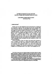
Structure of the book

. . . . . . . . . . . . . . . . . . . . . . . . . . . . . . . . xxiii

1.1 1.2

General form of a while program . . . . . . . . . . . . . . . . . . . . . . . . . . 10 The keywordwhile language as a kernel language . . . . . . . . . . . . . . . . . 25

2.1 2.2 3.1

A program trace for solving simultaneous equations on the Analytical Engine . 33 Some stages in the development of electronic universal machines . . . . . . . . . 35 √ A right-angled triangle with hypotenuse of length 2 . . . . . . . . . . . . . . . 70

4.1 4.2 4.3

A is a subalgebra of B . . . . . . . . . . . . . . . . . . . . . . . . . . . . . . . . 111 An impression of the idea of importing . . . . . . . . . . . . . . . . . . . . . . . 115 Architecture of the algebra AReals with Integer Rounding . . . . . . . . . . . . . . . . 121

5.1 5.2 5.3 5.4 5.5

One interface, many implementations. One signature, many algebras. A subclass K of the Σ -algebras satisfying properties in T . . . . . . . Classes of integer implementations. . . . . . . . . . . . . . . . . . . . Cyclic arithmetic. . . . . . . . . . . . . . . . . . . . . . . . . . . . . Integral domain specification. . . . . . . . . . . . . . . . . . . . . . .

. . . . .

. . . . .

. . . . .

. . . . .

. . . . .

. . . . .

129 130 132 133 140

6.1 6.2 6.3 6.4 6.5 6.6 6.7 6.8 6.9 6.10 6.11

A typical interactive system computing by transforming streams A dynamic 1-dimensional array . . . . . . . . . . . . . . . . . . Model of a finite array . . . . . . . . . . . . . . . . . . . . . . . Examples of models of discrete and continuous time . . . . . . Time modelled as cycles . . . . . . . . . . . . . . . . . . . . . . System with finite determinacy principle . . . . . . . . . . . . . Spaces and their coordinates . . . . . . . . . . . . . . . . . . . The effect of spatial object operations . . . . . . . . . . . . . . Operations on heart data visualising fibres . . . . . . . . . . . . Tree structure of a CVG term and the scene defined by it . . . Requirement for coordinate systems to be equivalent . . . . . .

. . . . . . . . . . .

. . . . . . . . . . .

. . . . . . . . . . .

. . . . . . . . . . .

. . . . . . . . . . .

. . . . . . . . . . .

. . . . . . . . . . .

. . . . . . . . . . .

158 164 166 173 174 177 185 193 196 197 202

7.1 7.2 7.3 7.4 7.5 7.6 7.7

Relating decimal to binary representations of the naturals . . . . . Relating binary to decimal representations of the naturals . . . . . Commutative diagram illustrating the Operation Equation . . . . . Preservation of operations under a homomorphism . . . . . . . . . Preservation of relations under a Boolean-preserving homomorphism Function f continuous on R . . . . . . . . . . . . . . . . . . . . . . Function f discontinuous at x = . . . , −1 , 0 , 1 , 2 , . . . . . . . . . . . .

. . . .

. . . . . . . . .

. . . . . . .

. . . . . . .

. . . . . . .

. . . . . . .

. . . . . . .

210 211 212 214 214 217 217

xiii

. . . . . . . . . .

xiv

LIST OF FIGURES 7.8 7.9 7.10 7.11 7.12 7.13 7.14

Machine S1 simulates machine S2 . . . . . . . . . A function and its inverse . . . . . . . . . . . . . Isomorphisms preserve operations . . . . . . . . . The class of all Σ Naturals -algebras . . . . . . . . . Tracking functions simulating the operations of A The image im(φ) of a homomorphism φ . . . . . First Homomorphism Theorem . . . . . . . . . .

. . . . . . .

. . . . . . .

. . . . . . .

. . . . . . .

. . . . . . .

. . . . . . .

. . . . . . .

. . . . . . .

. . . . . . .

. . . . . . .

. . . . . . .

. . . . . . .

. . . . . . .

. . . . . . .

. . . . . . .

. . . . . . .

. . . . . . .

221 224 225 235 237 240 245

8.1 8.2 8.3 8.4 8.5 8.6

Examples of basic formulae . . . . . . . . . . . Tree representation of some terms of the algebra Tree representation of some terms of the algebra Tree representation of some terms of the algebra The tree Tr (f (t1 , . . . , tn )) . . . . . . . . . . . . The many-sorted tree Tr s (f (t1 , . . . , tn )) . . . .

. . . . . . . . . . T (Σ Naturals1 , ∅) . T (Σ Naturals1 , X ) T (Σ Nat+Tests , X ) . . . . . . . . . . . . . . . . . . . .

. . . . . .

. . . . . .

. . . . . .

. . . . . .

. . . . . .

. . . . . .

. . . . . .

. . . . . .

254 272 272 272 273 274

9.1

Dedekind’s continuity axiom

10.1 10.2 10.3 10.4 10.5 10.6 10.7 10.8 10.9

The upper-case alphabet of Attic Greek of the Classical Period. Designing a language . . . . . . . . . . . . . . . . . . . . . . . . ∗ ∗ Possible derivations from the grammar G 0 1 . . . . . . . . . . n n Possible derivations from the grammar G a b . . . . . . . . . . a 2n Possible derivations from the grammar G . . . . . . . . . . . Specifying a language using a grammar . . . . . . . . . . . . . Component grammars used to construct the grammar G while . . . Structure of addresses . . . . . . . . . . . . . . . . . . . . . . . Structure of http addresses . . . . . . . . . . . . . . . . . . . .

. . . . . . . . . . . . . . . . . . . . . . . . . . . . 301

11.1 Architecture of grammar for signatures without imports 11.2 Architecture of signatures with imports . . . . . . . . . 11.3 Signatures and modular signatures . . . . . . . . . . . . 11.4 Dependency graph . . . . . . . . . . . . . . . . . . . . . 11.5 Modular grammar for first order formulae specifications 11.6 Modular grammar for equational logic specifications . . 11.7 General structure of Euclid’s Algorithm . . . . . . . . . 11.8 Architecture of while programs over the natural numbers 11.9 Architecture of while programs over a fixed signature . 11.10Architecture of while programs over any data type . . .

. . . . . . .

. . . . . . . . . . . .

. . . . . . . . . .

12.1 12.2 12.3 12.4 12.5

The Chomsky hierarchy . . . . . . . . . . . . . . . . . . . . . 2n Equivalent grammars to generate the language La = {a i | i is n n n Derivation of aabbcc in the context-sensitive grammar G a b c n n n n n n Hierarchy of languages L(G a ), L(G a b ) and L(G a b c ) . . Derivation tree Tr for the string z = uvw . . . . . . . . . . .

13.1 13.2 13.3 13.4

Recognising Recognising Recognising Recognising

the letter ‘s’ . . . . . . . the letter ‘t’ . . . . . . . the string ‘st’ . . . . . . . and distinguishing between

. . . . . . . . . . . . . . . . . . . . . . . . . . . the strings ‘sta’

. . . . . . . . .

. . . . . . . . .

. . . . . . . . .

. . . . . . . . .

. . . . . . . . .

. . . . . . . . .

. . . . . . . . .

. . . . . . . . .

. . . . . . . . .

362 367 369 370 370 373 377 382 389

. . . . . . . . . .

. . . . . . . . . .

. . . . . . . . . .

. . . . . . . . . .

. . . . . . . . . .

. . . . . . . . . .

. . . . . . . . . .

. . . . . . . . . .

. . . . . . . . . .

402 405 407 410 415 419 422 423 435 441

. . . . even} . . . . . . . . . . . .

. . . . .

. . . . .

. . . . .

. . . . .

. . . . .

. . . . .

451 454 456 456 471

. . . .

. . . .

. . . .

. . . .

. . . .

. . . .

481 481 481 482

. . . . . . . . . .

. . . . . . . . . . . . . . . . . . and ‘sto’

. . . .

. . . .

xv

LIST OF FIGURES 13.5 Recognising and distinguishing between the strings ‘star’ and ‘stop’ . . . . . 13.6 Recognising and distinguishing between the strings ‘start’ and ‘stop’ . . . . 13.7 Recognising an arbitrary string a1 a2 · · · an . . . . . . . . . . . . . . . . . . . 13.8 Automaton for ‘start’ and ‘stop’ following the general technique . . . . . . . 13.9 A typical finite state automaton . . . . . . . . . . . . . . . . . . . . . . . . 13.10Finite state automaton that accepts the strings ‘start’ and ‘stop’ . . . . . . 13.11Automaton to recognise the numbers 1 to 3 . . . . . . . . . . . . . . . . . . 13.12Automaton to recognise the numbers 1 to 3 with a single final state . . . . 13.13Automaton to recognise the numbers 1 to 3 with merged transitions . . . . 13.14Automaton to recognise the numbers 0 , 1 , . . . , 999 . . . . . . . . . . . . . . ∗ 13.15Automaton M D to recognise strings of digits of length zero or more . . . . + 13.16Automaton M D to recognise strings of digits . . . . . . . . . . . . . . . . . 13.17Automaton M N+ recognises non-zero natural numbers . . . . . . . . . . . . 13.18Automaton M N to recognise numbers . . . . . . . . . . . . . . . . . . . . . 13.19Automaton to recognise strings ab, aabb, aaabbb and aaaabbbb . . . . . . . 13.20Automaton recognises infinite strings but without matching . . . . . . . . . 13.21Automaton recognises infinite strings with matching but in disturbed order 13.22Automaton with empty moves to recognise the language {a i b j | i , j ≥ 0 } . . 13.23Automaton without empty moves to recognise the language {a i b j | i , j ≥ 0 } 13.24Automaton M Z to recognise integers by re-using the automata M N and M N+ 13.25Flattened automaton M Flattened Z to recognise integers . . . . . . . . . . . . 13.26Modular automaton to recognise program identifiers . . . . . . . . . . . . . 13.27Flattened automaton M Flattened Identifier to recognise program identifiers . . . 13.28Deterministic automaton to recognise the language {a i b j | i , j ≥ 0} . . . . . 13.29Translation of rules of the form A → a . . . . . . . . . . . . . . . . . . . . . 13.30Translation of rules of the form A → Ba or A → aB . . . . . . . . . . . . . 13.31Simulation automaton for G Regular Number . . . . . . . . . . . . . . . . . . . . 13.32Path chosen through the automaton to recognise the string z = uvw ∈ L . . 13.33Empty set finite state automata . . . . . . . . . . . . . . . . . . . . . . . . 13.34Empty string finite state automata . . . . . . . . . . . . . . . . . . . . . . . 13.35Single terminal symbol finite state automata . . . . . . . . . . . . . . . . . 13.36Concatenation operation on finite state automata . . . . . . . . . . . . . . . 13.37Union operation on finite state automata . . . . . . . . . . . . . . . . . . . 13.38Iteration operation on finite state automata . . . . . . . . . . . . . . . . . . 13.39Automaton to recognise the language {a i b j | i , j ≥ 0} . . . . . . . . . . . . 13.40Regular expressions associated with paths through the automaton . . . . . . Tree for the derivation of the string aaabbb from the grammar G ab . . Representation of the application of a production rule A → X1 X2 · · · Xn Derivation sub-tree for production rule A → a1 . . . an . . . . . . . . . . Derivation sub-tree for production rule A → u0 A1 u1 · · · un−1 An un . . . Derivation trees for Examples 10.2.2(1) . . . . . . . . . . . . . . . . . Derivation trees for Examples 10.2.2(2) . . . . . . . . . . . . . . . . . Derivation trees for Examples 10.2.2(3) . . . . . . . . . . . . . . . . . Derivation trees for generating Boolean expressions . . . . . . . . . . . Derivation tree for the program statement x :=y; y :=r; r :=x mod y . .

14.1 14.2 14.3 14.4 14.5 14.6 14.7 14.8 14.9

. . . . . . . . . . . . . . . . .

. . . . . . . . .

. . . . . . . . . . . . . . . . . . . . . . . . . . . . . . . . . . .

. . . . . . . . . . . . . . . . . . . . . . . . . . . . . . . . . . . .

483 483 484 484 486 488 490 491 491 492 493 494 495 495 497 498 499 501 503 506 507 509 510 513 517 517 521 527 532 532 533 534 535 536 539 540

. . . . . . . . .

. . . . . . . . .

546 547 547 548 550 551 552 552 554

xvi

LIST OF FIGURES

14.10Two derivation trees for the string ab . . . . . . . . . . . . . . . . . . . . . . . 556 14.11Derivation trees produced by the ambiguous BNF DanglingElse . . . . . . . . . 557 14.12Derivation tree produced by the unambiguous BNF MatchElseToClosestUnmatchedIf 560 14.13Derivation trees for the string true and false and not true from original grammar and its CNF variant 57 14.14Derivation trees for the string true and false and not true from original grammar and its GNF variant 58 14.15Derivation tree Tr for the string z = uvwxy . . . . . . . . . . . . . . . . . . . . 592 14.16Architecture of while programs over the natural numbers with declarations . . 595 15.1 15.2 15.3 15.4 15.5 15.6 15.7 15.8

Parsing abstract syntax and unparsing concrete syntax . . . . . . . . . . . . . Possible relationships between abstract syntax, concrete syntax and semantics Abstract syntax tree for the program x :=y; y :=r; r :=x mod y . . . . . . . . The algebra WP(Σ ) of while commands with definitions of operations . . . . The tree representation of the term x2 :=3; skip . . . . . . . . . . . . . . . . The tree representation of the term while not x0 = 2 do x0 :=x0 + 1 od . . . Pretty-printing from abstract syntax to concrete syntax . . . . . . . . . . . . Derivations and algebraic trees and terms of sample phrases . . . . . . . . . .

. . . . . . . .

610 610 611 617 619 619 620 635

16.1 Extending the kernel while language . . . . . . . . . . . . . . . . . . . . . . . . 649 16.2 The store modelled by state σ . . . . . . . . . . . . . . . . . . . . . . . . . . . . 658 18.1 18.2 18.3 18.4

Execution trace for Euclid’s algorithm . . . . . . . . . . . . . . . . . . . . . . . 711 Derivation trace for Euclid’s algorithm using structural operational semantics . 716 Semantic kernel of a language . . . . . . . . . . . . . . . . . . . . . . . . . . . . 717 Semantic kernel of while programs . . . . . . . . . . . . . . . . . . . . . . . . . 719

19.1 19.2 19.3 19.4

Form of register machine . . . . . . Data registers ρD ∈ Reg D of the VR Test registers ρB ∈ Reg B of the VRM Virtual machine instructions . . . .

. . . .

. . . .

. . . .

. . . .

. . . .

. . . .

. . . .

. . . .

. . . .

. . . .

. . . .

. . . .

. . . .

. . . .

. . . .

. . . .

. . . .

. . . .

. . . .

. . . .

. . . .

. . . .

. . . .

. . . .

727 729 730 731

20.1 The correctness of a compiler for a single program P ∈ Prog S . . . . . . . . . . 748 20.2 Compiler correctness for input-output semantics . . . . . . . . . . . . . . . . . 749 20.3 Compiler correctness for operational semantics . . . . . . . . . . . . . . . . . . 750 21.1 Execution of compiled sequenced statements . . . . . . . . . . . . . . . . . . . . 772 21.2 Execution of compiled conditional statements . . . . . . . . . . . . . . . . . . . 773 21.3 Execution of compiled iterative statements . . . . . . . . . . . . . . . . . . . . . 775

List of Tables 14.1 Machine characterisations of languages . . . . . . . . . . . . . . . . . . . . . . . 587 16.1 An example of real -sorted and Bool -sorted states. . . . . . . . . . . . . . . . . 659 16.2 New state after substitution . . . . . . . . . . . . . . . . . . . . . . . . . . . . . 660

xvii

xviii

LIST OF TABLES

xix

PREFACE

Preface Data, syntax and semantics are among the Big Ideas of Computer Science. The concepts are extremely general and can be found throughout Computer Science and its applications. Wherever there are languages for specifying, designing, programming or reasoning, one finds data, syntax and semantics. A programming language is simply a notation for expressing algorithms and performing computations with the help of machines. There are many different designs for programming languages, tailored to the computational needs of many different types of users. Programming languages are a primary object of study in Computer Science, influencing most of the subject and its applications. This book is an introduction to the mathematical theory of programming languages. It is intended to provide a first course, one that is suitable for all university students of Computer Science to take early in their education; for example, at the beginning of their second year, or, possibly, in the second half of their first year. The background knowledge needed is a first course in imperative programming and in elementary set theory and logic. The theory will help develop their scientific maturity by asking simple and sometimes deep questions, and by weaning them off examples and giving them a taste for general ideas, principles and techniques, precisely expressed. We have picked a small number of topics, and attempted to make the book self-contained and relevant. The book contains much basic mathematical material on data, syntax and semantics. There are some seemingly advanced features and contemporary topics that may not be common in the elementary text-book literature: data types and their algebraic theory, real numbers, interface definition languages, algebraic models of abstract syntax, use of algebraic operational semantics, connections with computability theory, virtual machines and compiler correctness. Where our material is standard (e.g., grammars), we have tried to include new and interesting examples and case studies (e.g., internet addressing). The book is also intended to provide a strong foundation for the further study of the theory of programming languages, and related subjects in algebra and logic, such as: algebraic specification; initial algebra semantics; term rewriting; process algebra; computability and definability theory; program correctness logic; λ-calculus and type theory; domains and fixed point theory etc. There are a number of books available for these later stages, and the literature is discussed in a final chapter on further reading. The book is based on the lectures of J V Tucker (JVT) to undergraduates at the University of Leeds and primarily at the University of Wales Swansea. In particular, it has developed from the notes for a compulsory second year course on the theory of programming languages, established at Swansea in 1989. These notes began their journey from ring binder to book-shop in 1993, when Chris Tofts taught the course in JVT’s stead, and provided the students with a typescript of the lecture notes. Subsequently, as JVT continued to teach the course, Karen Stephenson (KS) maintained and improved the notes, and assisted greatly in the seemingly endless process of revision and improvement. She also contributed topics and conducted a number of successful experiments on algebraic methods with the students. KS became a coauthor of the book in 2000. Together, we revised radically the text and added new chapters on regular languages, virtual machines and compiler correctness. JVT’s interest and views on the theory of programming languages owe much to J W de Bakker, J A Bergstra and J I Zucker. Ideas for this book have been influenced by continuous conversa-

xx

PREFACE

tions and collaborations starting at the Mathematical Centre (now CWI), Amsterdam in 1979. However, its final contents and shape has been determined by our own discussions and our work with several generations of undergraduate students. We would like to thank the following colleagues at Swansea: Dafydd Rees, Chen Min, Jens Blanck, Andy Gimblett, Neal Harman, Chris Whyley, Oliver Kullmann, Peter Mosses, . . . for their reading of selected chapters, suggestions and advice. A special debt is owed to Markus Roggenbach for a reflective and thorough reading of the text. We are grateful to the following students who formed a reading group and gave useful criticism of earlier drafts of the text: Carl Gilbert, Kevin Hicks, Rachel Holbeche, Tim Hutchison, Richard Knuszka, Paul Marden, Ivan Phillips and Stephan Reiff. We are grateful to Hasib Kabir Chowdhury who, as a student, read a later version of the manuscript and made many suggestions. Our colleagues and students have made Swansea a warm and inspiring environment in which to educate young people in Computer Science. The ambiguities and errors that remain in the book are solely our responsibility.

J V Tucker Perriswood, Gower, 2003 K Stephenson Malvern, 2003

xxi

A GUIDE FOR THE READER

A Guide for the Reader The educational objectives of the book are as follows: Educational Objectives 1. To study some theoretical concepts and results concerning abstract data types; programming language syntax; and programming language semantics. 2. To develop mathematical knowledge and skills in mathematically modelling computing systems. 3. To introduce some of the intellectual history, technical development, organisation and style of the scientific study of programming languages. At the heart of the book is the idea that the theory presented is intended to answer some simple scientific questions about programming languages. A long list of scientific questions is given in Section 1.2. To answer these questions we must mathematically model data, syntax and semantics, and analyse the models in some mathematical depth. In addition to meeting the objectives above, we hope that our book will help the students learn early in their intellectual development the following: Intellectual Experiences 1. That the mathematical theory gives interesting and definitive answers to essential questions about programming. 2. That the theory improves the capacity for practical problem solving. 3. That the answers to the scientific questions posed involve a wide range of technical material, that was invented and developed by many able people over most of the twentieth century, and has its roots in the nineteenth century. 4. That the theory contains technical ideas that may be expected to be useful for decades if not centuries. 5. That intellectual curiosity and the ability to satisfy it are ends in themselves. It will be helpful to summarise the structure and contents of the book, part by part, to ease its use by the reader, whether student or teacher.

Subjects Data, syntax and semantics are fundamental and ubiquitous in Computer Science. This book introduces these three subjects through the theoretical study of programming languages. The subjects are intimately connected, of course, and our aim is to integrate their study through the course of the whole book. However, we have found it natural and practical to divide the text into three rather obvious parts, namely on data, syntax and semantics. We begin with a general overview of the whole subject, and a short history of the development of imperative programming languages.

xxii

A GUIDE FOR THE READER

Part I is on data. It is an introduction to abstract data types. It is based on the algebraic theory of data and complements their widespread use in practice. We cover many examples of basic data types, and model the interfaces and implementations of arbitrary data types, and their axiomatic specifications. We focus on the data types of the natural numbers and real numbers, data in time and space, and terms. Part II is on syntax. It introduces the problem of designing and specifying syntax using formal languages and grammars, and it develops a little of the theory of regular and context free grammars. Again, there are plenty of examples to motivate and illustrate the language definition methods and their mathematical theory. Our three main case studies are simple but influential: addresses, interface definition languages and imperative programming languages. We round off the topic by applying data type theory to abstract syntax and the definition of languages. Part III is on semantics. It introduces some methods for defining the semantics of imperative programs using states and their transformation. It also deals with proving properties of programs using structural induction. We conclude with a study of compiler correctness. We define a simple virtual machine and compiler from an imperative language into its virtual assembler and prove by structural induction that it is correct. In the book explanations are detailed and examples are abundant. There are plenty of exercises, both easy and hard, including some longer assignments. The final chapter of each part contains advanced undergraduate material that brings together ideas and results from earlier chapters. Occasionally, sections in other chapters will also contain such advanced material. We will mark chapters and sections with advanced material using *.

Options Rarely are the chapters of a scientific textbook read in order. Lecturers and students have their own ideas and needs that lead them to re-order, select or plunder the finely gauged writings of authors. This textbook presents a coherent and systematic account of the theory of programming languages, but it is flexible and can be used in several ways. We certainly hope the book will be plundered for its treasures. A selection of materials to support courses based on the book can be found on the web site: http://www... The structure of the book is depicted in Figure 1, which describes the dependency of one chapter upon another. The chapters may be read in a number of different orders. For example, all of Part I can be read independently of Part II, but Chapter 16 of Part II depends on Chapters 3–6 of Part I. The complete course can be given by reading all the chapters in order. As noted, it is easy to swap the order of Part I and Part II. A concise course that covers the mathematical modelling of an imperative language with arbitrary data types, but without the advanced topics, can be based on this selection of chapters: Data

Chapters 1, 3–7

xxiii

A GUIDE FOR THE READER Welcome introduction 1

I: Data Core

2 history II: Syntax

algebras 3

grammars 10

interfaces 4

examples 11

specifcations 5

III: Semantics 16 input-output semantics 17 structural 18 operational semantics induction

regular 12 languages

data structures 6

context

homomorphisms 7

19 virtual machines

free 14 13 languages

20 compiler correctness

abstract 15 syntax

21 compiler verification

finite state automata

terms 8

Advanced real numbers 9

further reading 22

Figure 1: Structure of the book.

Syntax

Chapters 10–14

Semantics Chapters 16 and 17 Shorter and easier courses are also practical: Data

Chapters 1, 3–6

Syntax

Chapter 10 and 11

Semantics Chapters 16 and 18 A set of lectures on data types can be based on: Data

Chapters 3–9

Syntax

Chapter 15

Semantics Chapter 16 and 17 A set of lectures on syntax can be based on: Data Chapters 3–4

xxiv

A GUIDE FOR THE READER Syntax Chapters 10–15

A set of lectures on hierarchical structure and correct compilation can be based on: Syntax Chapter 10 and 11. Semantics Chapter 16–17 and 19–21.

Prerequisites Throughout, we assume that readers have a sound knowledge and experience of (i) programming with an imperative language; (ii) sets, functions and relations; (iii) number systems and induction; (iv) propositional and predicate logic; and (v) axioms and deduction. However, our chapters provide plenty of reminders and opportunities for revising these essential subjects. Students who take the trouble to revise these topics thoroughly, here at the start, or even as they are needed in the book, will progress smoothly and speedily. Occasionally, for certain topics, we will use or mention some more advanced concepts and results from abstract algebra, computability theory and logic. Hopefully, these ideas will be clear and only add to the richness of the subject.

Notation We will follow the discipline of mathematical writing, adopting its standard notations, forms of expression and practices. It should be an objective for the student of Computer Science to master the elements of mathematical notation and style. Notation in Computer Science is very important and always complicated by the need for concepts to have three forms of notation: Mathematical Notation is designed to facilitate mathematical expression and analysis of general ideas and small illustrative examples; Descriptive Notation is designed to facilitate reading and comprehension of large examples and case studies; and Machine Notation is designed to facilitate processing by machine. Several of our key concepts (algebras, grammars, programs, etc.) will be equipped with two standard notations aimed at the Mathematical Notation and Descriptive Notation.

xxv

A GUIDE FOR THE READER

Exercises and Assignments At the end of each chapter there is a set of problems and assignments designed to improve and test the student’s understanding and technique. Some have been suggested by students. The problems illustrate, complete, explore, or generalise the concepts, examples and results of the chapter.

Revision We end this Guide with an assignment that invites students to revise the prerequisites and with a piece of advice: do this assignment, and do it well. Prepare a concise list of concepts, notations and results that you believe are the basics of the five topics mentioned in the Prerequisites. Add to this list as you study the following chapters. Here is a start. Programming variable expression assignment sequencing conditional branching iteration procedure array, list, queue, stack .. . Sets ∅ x ∈A A⊆B A∪B A−B |A|

A 6= ∅ x 6∈ A A 6⊆ B A∩B P(A) .. . Functions

f g f f f f f

:A→B ◦ f : A → C where f : A → B and g : B → C . is total. is partial. is injective, or one-to-one. is surjective, or onto. is bijective, or a one-to-one correspondence. .. .

xxvi

A GUIDE FOR THE READER Relations R ⊂A×B ≡ equivalence relation ≤ partial order ≤ total order

xRy [a] equivalence class .. .

Number Systems N Z Q R

natural numbers integers rational numbers real numbers Logic p∧q p∨q p⇒q ¬p ∀x : R(x ) ∃x : R(x )

Axiomatic Theory definition axiom postulate law lemma theorem corollary proof deduction counter-example conjecture .. .

Welcome

1

Chapter 1 Introduction Data, syntax and semantics are three fundamental ideas in Computer Science. They are Big Ideas. That is: they are ideas that are general and widely applicable; they are deep and are made precise in different ways; they lead to beautiful and useful theories. The ideas are present in any computing application. As its contributions to Science and human affairs mature, Computer Science will influence profoundly many areas of thinking, making and doing. Thus data, syntax and semantics are three ideas which are fundamental in Science and other intellectual fields. Our introduction to these concepts of data, syntax and semantics is through the task of modelling and analysing programming languages. Programming languages abound in Computer Science and range from large general purpose languages to the small input languages of application packages. Some languages are well known and widely used, some belong to communities of specialists, some are purely experimental and do not have a user group. The number of programming languages cannot be counted! In learning a programming language the aim is to read, write and execute programs. A programmer should understand the organisation and the operation of the program, and be able to predict and test its input-output behaviour, to know, for example, if the program computes a specified function. After gaining fluency in one or more programming languages it is both natural and necessary to reflect on the components that make up the languages and enquire about their individual roles and properties. A multitude of questions can be formulated about the capabilities and shortcomings of a language and its relation with other languages. For example, How is this programming language specified? and Is this language more powerful than that? To awaken the reader’s curiosity, we will ask many questions like these shortly, in Section 1.2. To understand something of the nature and essential elements of programming languages, we will look at their overall structure and separate components rather abstractly and analytically, and answer some of these questions. Now, this analysis, comparison and classification of language components requires a large scale scientific investigation. The investigation is organised as the study of three aspects of programs: Data

the information to be transformed by the program

Syntax

the text of the program

Semantics the behaviour of the program To create a theory of programming languages we need to discover fundamental concepts, meth1

2

CHAPTER 1. INTRODUCTION

ods and results that can reveal the essential structure of programming languages, and can answer our questions. In this first chapter we will simply prepare our minds for theoretical investigations. We will explore the scientific view of programming languages (Section 1.1) raise plenty of questions about programming languages for which we need answers (Section 1.2), and look at some raw material for modelling programming languages (Section 1.3). We will focus on the theory of programming in the small and have only occasional encounters with programming in the large. Measured against the state of contemporary language technology, our scientific goal seems modest indeed: To understand the general principles, structure and operation of imperative programs that compute functions on any kind of data. Yet attaining this goal will bring rich rewards.

1.1

Science and the aims of modelling programming languages

Computing systems are artificial. They are designed and developed by and for human use. They are superseded and are discarded, sometimes with uncomfortable speed. Some are publically managed and some are commercial products. However, the scientific study of computing systems is remarkably similar to the scientific study of physical systems which are God given and timeless. Roughly speaking, scientific studies have theoretical and practical objectives, pursue answers to definite questions, and require mathematical models and experimental methods. Theoretical Computer Science develops mathematical models and theories for the design and analysis of • data; • specifications of computational problems with data; • algorithms for transforming data; • programs and programming languages for expressing algorithms; • systems and machine architectures for implementing programming languages. Simply put, the subject is aimed towards the discovery and application of fundamental principles, models, methods and results, which are intended • to help understand the nature, scope and limits of computing systems; • to help software and hardware engineers make computing systems. Fundamentally, Theoretical Computer Science is speculative. It thrives on curiosity and the freedom to imagine, idealise and simplify. Theoretical Computer Science creates ideas for new data types and applications, new ways of specifying, programming and reasoning, and new

1.2. SOME SCIENTIFIC QUESTIONS ABOUT PROGRAMMING LANGUAGES

3

designs for machines and devices. For example, over the past decades, theorists have been thinking about new ways of doing exact calculations with real numbers, the integration of simulated and experimental data in virtual worlds, languages for specifying and programming distributed and mobile devices, ways of modelling and proving concurrent systems correct, asynchronous designs for chips, and quantum and biological computers. In time, some theories become the foundations of mature technologies, whilst others stubbornly resist practical or commercial exploitation. Theoretical Computer Science also has many problems that retain importance long after the technology is established. The theory of programming languages is laden with such legacy problems: the theories of types, concurrency, objects, agents are rich in difficulties and mysteries, both conceptual and mathematical. Theories of programming languages and program construction are a fundamental area of Theoretical Computer Science. There are many programming constructs and program development techniques and tools, all of which are the fruits of, or require, theoretical investigation. In our time, it is believed widely that the development of theories is necessary for the practical craft of program construction to become a mathematically well-founded engineering science. Independently of such a goal, we believe that the development of theories is necessary to satisfy our curiosity and to understand what is being done, what could be done, and how to do better. The scientific approach of the theory of programming languages places three intellectual requirements on the reader: Intellectual Aims 1. To ask simple questions. 2. To make and analyse simple mathematical models. 3. To think deeply and express ideas precisely. Now we will formulate a number of questions and set the scene for some mathematical theories to answer them. Our theories will show how it is possible • to model mathematically any kind of data; • to model mathematically the syntax of a programming language; • to model mathematically the semantics of a programming language.

1.2

Some Scientific Questions about Programming Languages

Let us begin by posing some simple questions about a programming language. The questions will make us reflect on our ideas about programming languages and programs. They require us to think generally and abstractly. They also require us to explore our existing knowledge, experience and prejudices.

4

CHAPTER 1. INTRODUCTION

This is part of the raw material from which theories are made. Most of the questions we pose are insufficiently precise to allow a definite answer. Thus, one of our most important tasks will be to make questions precise, using mathematical models, and hence turn them into technical problems that can be solved definitively. By no means all of the questions will be given an answer in this book: readers are invited to return to this section from time to time to see which questions they can formulate and answer precisely. Let L and L0 be any programming languages, real or imaginary. Try to answer the following seemingly vague questions. Data What is data and where does it come from? How do we choose operations on data? How do we compare the choice of different sets of operations? How do we know we have enough operations on data? What exactly are data types? What is an interface to a data type? What is an implementation of a data type? How do we specify data types like integers, reals or strings, independently of programming languages? How do we model data types for users’ applications? To what extent is a data type independent of its implementation? How do we compare two implementations of a data type? Can any data type be implemented using an imperative language? Are the representations of the natural numbers based upon decimal, binary, octal and Roman notations equivalent? How accurate as approximations are implementations of the real numbers? What are the effects of approximating infinite sets of data by finite subsets? Are error messages necessary for data types? What are the base data types of L? What data types can be implemented in L? Can any data type be implemented in L? Syntax What is syntax and why is there so much of it? Is any notation a syntax? How do we choose and make a syntax using symbols and rules? How do we check for errors in syntax? How do we transform program syntaxes, as in substitution and expansion, compilation and interpretation? How do we specify and transform texts for pretty printing, internet publication and slide projection? What are the syntactic categories such identifiers, types, operations, declarations, commands, and procedures, classes? What are scope and binding rules? What are the benefits of prefix, infix, postfix, or mixfix notations? How do we define exactly the syntax of L? How do we specify the set of legal programs of L? Is there an algorithm that checks that the syntax of a program of L is correct? Semantics What is semantics? Why do we need to define behaviour formally? How do we choose one from the many possible semantics for a construct? Is there a “right” semantics for every construct? What is input-output behaviour? What are deterministic and nondeterministic behaviours? Can every partial function be extended to a total function by adding an undefined flag? How do we model the behaviour of any program containing while, goto, and recursion? Can one use tests that return a “don’t know” flag? What happens when a program raises an exception? How

1.2. SOME SCIENTIFIC QUESTIONS ABOUT PROGRAMMING LANGUAGES

5

do procedures work? What is encapsulation and information hiding? What is parallel execution and concurrent communication? What are type systems, classes and objects, inheritance and polymorphism? What is a program library? How do we define exactly the semantics of L? How do we specify the meaning of the data types and commands of L? How do we specify the operation or dynamic behaviour of programs of L? How do we specify the input-output behaviour of programs required by users? What is a program trace? What is the relationship between the number of steps in a computation and its run time? What exactly does it mean for two programs of L to be equivalent? Expressiveness and Power How expressive or powerful is L? Can L implement any desired data type, function or specification? Which specifications cannot be implemented in L? Is L equally expressive as another programming language L0 ? There are four possibilities: • L and L0 are equivalent; • L can accomplish all that L0 can and more; • L0 can accomplish all that L can and more; or • L can accomplish some tasks that L0 cannot, and L0 can accomplish some tasks that L cannot. What exactly does it mean for two languages L and L0 to be equivalent in expressiveness or power? Which are the most expressive, imperative, object-oriented, functional or logic programming languages? Are parallel languages more expressive than sequential languages? Is L a universal language, i.e., can it implement any specification that can be implemented in some other programming language? Do universal languages exist? What is the smallest set of imperative constructs necessary to make a universal language? Program Properties What properties of the programs of L can be specified? Are there properties that cannot be specified? What exactly are static and dynamic properties? What properties of the programs of L can be checked by algorithms? What properties are decidable, or undecidable, when the program is being compiled? What properties are decidable, or undecidable, when the program is being executed? What is the relationship between the expressiveness or power of the language L and its decidable properties? What properties of programs in L can be proved? Given a program and an identifier, can we decide whether or not (i) the identifier appears in the program? (ii) given an input, the identifier changes its value in the resulting computation? (iii) the identifier changes its value in some computation? Given a program and an input, can we decide whether or not the program halts when executed on the input? Given two programs, can we decide whether or not they are equivalent?

6

CHAPTER 1. INTRODUCTION

Correctness How do we specify the purpose of a program in L? To what extent can we test whether or not a program of L meets its specification? How do we prove the correctness of a program with respect to its specification? Given a specification method, are there programs that are correct with respect to a specification but which cannot be proved to be correct? Is there an algorithm which, given a specification and a program, decides whether or not the program meets its specification? Compilation What exactly is compilation? How do we structure a compiler from the syntax of L to the syntax of L0 ? What does it mean for a compiler from L to L0 to be correct? Is correctness defined using a class of specifications, or by comparing the semantics of L and L0 ? How do we prove that a compiler from L to L0 is correct? Efficiency Are the programs of L efficient for a class of specifications? If L and L0 are equally expressive will the programs written in them execute equally efficiently? Can L be compiled efficiently on a von Neumann machine and is the code generated efficient? Are imperative programming languages more efficient than logic and functional languages? Are programs only involving while and other so-called structured constructs, less efficient than those allowing gotos? Are parallel languages more efficient than sequential languages? Attempting to answer the questions should reveal what the reader knows about programming languages, before and after studying this book.

1.3

A Simple Imperative Programming Language and its Extensions

Clearly, the questions of Section 1.2 are a starting point for a major scientific investigation, one that is ongoing in the Computer Science research community. We will examine only some of the questions by analysing in great detail an apparently simple imperative language. Definition (Imperative Language) An imperative language is based on the idea of placing data in a store and having commands or instructions that act on the store, creating and testing data, and moving it around the store. In summary, Imperative Program = Data + Store + Algorithm The language we will use for theoretical analysis is called the language WP of while programs with user-defined data types.

1.3. A SIMPLE IMPERATIVE PROGRAMMING LANGUAGE AND ITS EXTENSIONS 7 The main features of WP are its very general data types and very limited control constructs. The language WP can compute on any data but the most complicated control construct is the while loop. The language can be extended in many ways and is valuable as a kernel language, from which equally expressive but more convenient languages can be made by adding new constructs.

1.3.1

What is a while Program?

In our language WP , a program is created using (i) some data equipped with some atomic operations and tests; (ii) some store containing data; and (iii) some algorithm that uses these atomic operations and tests on the store. We combine the data and the given operations, and form a programming construct called a data type. The statements of a program invoke operations and tests via an interface for a data type. A program is a text composed of atomic statements that are scheduled by control constructs. The atomic statements are assignments that both compute and store the values of expressions made from the given atomic operations on data. The control constructs use tests made from the given Boolean-valued operations on data. Thus, we have an apparently simple idea of a program, namely: Imperative Program = Data Type + Store + Algorithm on Store In particular, in the language WP of while programs we carefully separate data from the store and the algorithm. This means we can study data independently of the core imperative programming constructs which involve the store. This is an important act, and is an example of a general idea: Working Principle Separate concerns, isolate concepts and study them independently. What do the programs of our language WP look like? Here is an example of a while program expressing a famous ancient algorithm:

8

CHAPTER 1. INTRODUCTION program

Euclid

signature

Naturals for Euclidean Algorithm

sorts

nat,bool

constants 0: →nat; true,false: →bool operations mod: nat × nat→nat; 6= : nat × nat→bool endsig body var

x,y,r: nat

begin read (x,y); r:=x mod y; while r 6= 0 do x:=y; y:=r; r:=x mod y od; write (y) end Euclid’s algorithm computes the greatest common divisor of two natural numbers. Let us examine its form and constructs (we consider its computational behaviour later, in Chapter 16). The form of the program is two parts with three components in total. Interface The first part is an interface for a data type which is called a signature. Specifically, it is: (i) a declaration listing names for the data and names for the operations on data. Body The second part is an algorithm that uses the data store which is called a body. Specifically, the body is:

1.3. A SIMPLE IMPERATIVE PROGRAMMING LANGUAGE AND ITS EXTENSIONS 9 (ii) a declaration of variables and their types which specifies a store or memory for the data of the data type; and (iii) a list of commands expressing the algorithm, which uses operations from the data type interface (i) and variables from the declarations (ii). The constructs of the program are of two kinds. First, there are commands that (a) apply operations on data that compute new data from old, and (b) store and transfer data. For example, the assignments: z:=x mod y and x:=y can combine the computation and storage of data. Secondly, there are commands that (c) apply operations on data that test data and control the order of execution of commands. For example, while z 6= 0 do . . . od The program is a list of instructions that we will call commands

or statements.

The list is built by placing the commands in order using the construct of sequencing denoted by ; and usually introducing a new line of text. However, the list has some nesting. Notice that the while construct “contains” a block of three sequenced commands. Finally, notice that the program obeys the conventions that the algorithm uses operations and variables that are declared inside the program. Next we will describe the general form of a while program and the constructs that form the core of the language. These observations on the structure of Euclid’s algorithm are merely the beginning of our search for general principles, theories and tools for building programming languages. On the basis of this example, possibly complemented by a few more, is it possible to gain a clear picture of what our while programs look like and to describe what they do? On the basis of examples, it is possible to recognise, adapt and create many new examples of while programs. This is how most people learn and hence “know” a programming language! However, it is not possible on the basis of examples, to even recognise all while programs since it is not possible to define exactly what is, and what is not, a while program. It is not possible to give exact rules, derived from or at least supported by general principles, for the composition of its programs. It is not possible to write an algorithm that would check the correctness of the program syntax (as we find in compilers). Clearly, on the basis of examples, it is not possible to answer the demanding questions we posed in Section 1.2. Working Principle Examples must be complemented by general concepts and principles.

10

CHAPTER 1. INTRODUCTION

1.3.2

Core Constructs

Let us review and formulate in more general terms some of the observations we made in the previous section. Program Structure The general form of a while program over a data type is summarised in Figure 1.1. program



signature endsig body



variables



begin

end



Figure 1.1: General form of a while program. It has the form Program = Data Type + while Program Body We concentrate on the elements of the components. More precisely, the principal constructs of the while language WP are as follows: Data Any set of data, and any operations and tests on the data, can be defined. Data, and operations and tests on data together form a data type. The interface by which the algorithm of a while program invokes a data type is called a signature and has the form:

1.3. A SIMPLE IMPERATIVE PROGRAMMING LANGUAGE AND ITS EXTENSIONS11 signature

a data type

sorts

. . . , s, . . . , bool

constants . . . , c :→ s, . . . operations . . . , f : s1 × · · · × sn → s, . . . . . . , r : s1 × · · · × sm → bool . . . endsig Here sorts are names for the sets of data, constants are names for special data and operations are names for functions and tests. Note that Booleans are needed for the tests. Variables and State For an imperative language, there are infinitely many variable names available, e.g., x0 , x 1 , x 2 , . . . also denoted a, b, c, . . . , m, n, . . . , x, y, z, . . . etc. when convenient. Normally, only finitely many variables are used in a program. The variables name “locations” in which to “store” data. The variables give rise to a notion of state of a store, memory and, indeed, computation. A state is a list of data recording what data is to be found in the locations named by the variables. The algorithm changes these states as its statements change data and locations. Thus, a computation can be seen as a sequence σ0 , σ 1 , . . . , σ t , . . . of states produced by the algorithm step by step in time. Atomic Statements An expression e, built from the variables and operators of the data type, can be evaluated and the result taken to be the new value of any variable x by an Assignment x :=e. We will also often include a dummy atomic statement which does nothing: Null

skip

For many purposes, skip is equivalent to trivial assignments such as x :=x . Control Constructs The order of performing operations is controlled by three constructs: Given programs S0 , S1 , S2 and test b, we can construct the new programs: Sequencing S1 ;S2 Conditional if b then S1 else S2 fi Iteration

while b do S0 od

12

CHAPTER 1. INTRODUCTION

Statements A while program’s algorithm is built from atomic statements by the repeated application of control constructs. The theory of this small set of programming constructs will provide answers to many of the questions in Section 1.2, and be strong enough to serve as a theoretical foundation for much larger languages.

1.4

Where do we find while programs?

The answer is: Almost everywhere! The while language is a small language yet it captures the primary ideas of imperative programming, namely, that data is placed in a store and a sequence of commands calculate and transform the data in the store. Before we put imperative programming under the microscope, using the constructs of the while language, let us look at how these constructs are expressed in different ways in different programming languages. We consider procedures that express Euclid’s gcd algorithm, which we have already written as a while program. Our while language is a theoretical language designed to express examples clearly and be analysed theoretically by people. The texts below are from languages that are designed to code large applications and be processed by machines. In each case we have given function procedures rather than programs. To an experienced eye the variety is not surprising and the differences are negligible because the essential structure of each procedure — i.e., the basic operations and loop — is the same. These ideas are laid bare in our while language, though even in theoretical investigations there are plenty of variations of notations. However, in using procedures we do simplify comparisons by omitting other parts of a gcd program. For example, we have omitted input and output code, which (i) may belong the program (e.g., written using read and write constructs in Pascal), or (ii) may not belong to the program (e.g., imported from library classes in Java), or (iii) may not even belong to the language (e.g., in pure Algol 60, input and output was not specified and was in the hands of machine-specific routines, though some dialects offered read and write). Functional and logic languages implement computational loops in entirely different ways. There is no end to the variety of ways of programming. Thus, it is not always trivial to rewrite a simple gcd program in another language. To an inexperienced eye the variety may be daunting and the differences in appearance may be surprising. The potential variety of texts is enormous for there are hundreds of languages in which to write a gcd procedure. Imagine a hundred gcd procedures, in a hundred languages, with the same essential structure but different texts. Do we see them all as the really same? No. For it is a fact that, in practice, some we like and some we do not. There is something personal about languages and we can have extra difficulties in using languages we do not like. The syntax of a language is like the clothes worn by a person. Clothes combine a purpose and a style, and emphasise practicality or display. They are something we have chosen, or a social group has chosen for us. Often clothes matter even when they should not.

1.4. WHERE DO WE FIND WHILE PROGRAMS?

13

Finally, before we leave our luxurious island of theoretical programming languages, and swim in the sea of practical programming languages, to collect our specimens of gcd code, we must take one or two safety precautions. First, in our while language we can use any data by simply declaring a signature. The gcd algorithm works on natural numbers. However, in expressing the gcd algorithm in practical languages it is easier to use the “standard” data type of the integers. Thus, the procedures below all compute with integers and have been called IGCD for integer greatest common divisor. In the case of integers x and y, which may be negative, we define igcd (x , y) = gcd (|x|, |y|), where |x| =

(

x −x

if x > 0 ; if x < 0 .

This is the function on integers we expect to program. Second, basic operations on the integers, like the modulus function, not only have different notations in the different languages, but can produce different answers. This variation belongs to the topic of data type design, of course. So much for the “standard” data type of the integers! Thus, let us adopt one true standard convention of practical programming: caveat emptor i.e., let the buyer beware. The reader is invited to check how these fragments compute igcd outside the natural numbers.

1.4.1

Gallery of Imperative Languages

Some general purpose languages of historical interest are: Fortran 66, Fortran 77, Fortran 90, Algol 60, ALGOL 68, PL/I, Basic, Pascal, Modula-2, Ada, BCPL, B, C They are all imperative languages. Here are a few samples of gcd procedures taken from the list. Fortran 66 FUNCTION IGCD(X, Y) INTEGER X, Y, R 10 IF (Y.EQ.0) GOTO 20 R = MOD(X, Y) X = Y Y = R GOTO 10 20 IGCD = X RETURN END

14

CHAPTER 1. INTRODUCTION

Algol 60 BEGIN INTEGER x, y; INTEGER PROCEDURE igcd(x, y); VALUE x, y; INTEGER x, y: BEGIN INTEGER r; loop : IF y NOTEQUAL 0 THEN BEGIN r:= x REM y; x := y; y: = r; GOTO loop END; END; igcd := x END igcd; Pascal function igcd (x, y : integer) : integer; var r: integer; begin while y 0 do begin r:= x mod y; x:= y; y:= r end; igcd := x end {igcd} C int igcd(int x, int y) { while (y) { int r = x%y; x = y; y = r; }; return x; }

1.4. WHERE DO WE FIND WHILE PROGRAMS?

1.4.2

15

Pseudocode and Algorithms

Pseudocode is language for people to describe, explain, and discuss algorithms. It is simply a blend of programming constructs and natural language. A great deal of pseudocode is a blend of simple imperative constructs and English. Usually, the constructs are those we will meet in the while language and its extensions. Pseudocode is like natural language: it has well understood forms, and a core that can be described and even specified. But since its purpose is communication between people, it can change and extend itself to fit the problems at hand and the fashions of the day. Pseudocode originates and remains close to the ideas of Algol 60. One of the primary aims of the designers of Algol 60 was to provide a language for people to express elegantly and communicate clearly algorithms (see Chapter 2). This goal they achieved. As new algorithms and programming ideas are discovered new constructs are created. The best of them will end up in Pseudocode, long after their algorithms and languages have fallen into disuse.

1.4.3

Object-Oriented Languages

Object oriented imperative languages use the idea of objects to abstract from the idea of a program as combining data, a store and an algorithm. An object can be seen as a basic unit or component of a program, having its own data, store and algorithms. The objects’s algorithms implement procedures on the data and store of the object which are called methods. The program is built from a number of objects, specially written or taken from a library. With this view of program, the construction of new objects from given objects is fundamental and has led to the development of many different ideas of inheritance and polymorphism. A key idea is that the single monolithic store associated with a classical imperative program is broken up into independent pieces. Thus, the basic intuition of variables indicating registers in a single global store, where data can be placed and found, is removed from programming and replaced by a new basic but more abstract conception of objects. The idea of an object is struggling to find its most general form, applicable to declarative and other languages. For our imperative purposes, objects simply generalise and unify the ideas data types and procedures on the store. The objects are instanced by classes. Some general purpose languages object oriented languages are: Simula 66, Smalltalk, Eiffel, C++, Java, C# In object-oriented programming, methods generalise procedures and functions. Thus, we can add to our gallery of gcd code by rewriting the gcd procedure as a method in different object-oriented languages. The examples of gcd methods continue to make the point that the essential ideas of while programs are alive and well in contemporary object-oriented programming languages. The development of object-oriented programming languages has extended imperative programming. There is a new emphasis on programming in the large, through the ideas of class and operations on libraries of classes. Through not necessary for the purpose of the gallery, it is interesting to examine the classes where these methods reside. Immediately, we see differences. Are they superficial or deep? The differences are magnified by the fact that we are in the early stages of research into theoretical models of object-oriented programming. We do not understand the fundamental ideas fully,

16

CHAPTER 1. INTRODUCTION

not to mention the needlessly complex features that inhabit practical technologies. Computer scientists have been here before: once upon a time, there was little stability in the matter of the key imperative constructs. One thinks of the history of recursive procedures, for example. Some of these aspects will be discussed in Chapter 2. Let us continue our gallery of gcd code. One object-oriented sample will suffice. Java In Java, traditional functions and procedures, characteristic of mathematical operations, are written as static methods. Thus a simple re-programming of the gcd procedure in Java is public static int gcd(int x, int y) { while (x != 0) { int r = x % y; x = y; y = r; } return x; } The public refers to the access rules for objects and ensures that the method is generally available if placed in a public class. How can the gcd static method be inserted into a class? Perhaps, the basic ideas of object-oriented programming would be simply served by the idea of simply extending the standard Integer class, supplied with the language, with a gcd method. For example, we can write: public class GCDInteger extends Integer { public Integer gcd(Integer a) { int y = a.intValue(); int x = this.intValue(); while (y != 0) { int r = x % y; x = y; y = r; } return new Integer(x); } } The calculation is made with data of type int, but the data is presented to the class as Integer objects, thus conversion from Integer to int and back is included. Unfortunately, the Integer class is designated as final which means that, in Java, classes may not inherit from it. Hence, the above simple idea and neat text is not allowed. In fact to see our little gcd as a class, the next step is to create an independent public class.

1.4. WHERE DO WE FIND WHILE PROGRAMS?

17

public class GCD { private int a; public GCD(int b) { a = b; } public int gcd(int y) { int x = a; while (y != 0) { int r = x % y; x = y; y = r; } return x; } } Why this gcd should be such a palaver makes an interesting question about bindings.

1.4.4

Algebraic, Functional and Logic Languages

Algebraic, functional and logic languages are based on the idea that one computes solely with functions and relations on data. The functions and relations can be defined and combined in different ways. The model of computation underlying an algebraic, functional or logic programming language is (i) to declare a new function or relation which has certain properties in terms of other functions and relations; (ii) to evaluate the function and relation using deduction in a formal calculus. The language is called declarative because functions and relations are declared by properties that specify the functions and relations “axiomatically”. Specifically, there is no abstraction of a machine, with commands transforming states, involved in programming. The most important method of definition is to write formulae that a function must satisfy such as some algebraic equations, recursion equations, or Horn clauses. The formulae constitute a program that defines the function and its implementation solves the unknown function or relation in the equations or formulae. Algebraic languages (such as OBJ and Maude) are based on deductions that rewrite terms using algebraic substitutions and equations. Functional languages (such as SML and Haskell) are based on deductions in special formal calculi for reducing functional expressions, such as various lambda calculi. Logic languages (such as Prolog) are based on deductions in formal predicate calculi using proof rules, such as Horn clause logic. In practice, declarative languages can acquire some familiar imperative constructs such as the assignment and the while loop. They are often considered to be imperfections (as in SML) or advanced constructs (as in Haskell). One sample gcd in each of the three types of language will be sufficient.

18

CHAPTER 1. INTRODUCTION

Haskell The gcd function is predefined in Haskell. However, we can re-code it as follows. igcd :: igcd 0 0 igcd x y where

Integer -> Integer -> Integer = error "igcd 0 0 is undefined" = gcd (abs x) (abs y) gcd x 0 = x gcd x y = gcd y (rem x y)

Maude In the algebraic language Maude we can write a functional module. fmod GCD is protecting INT . op GCD : Int Int -> Int . vars x y : Int . eq GCD(x, 0) = x . ceq GCD(x, y) = gcd(y, x rem y) if y =/= 0 . endfm Prolog igcd(X, 0, X). igcd(X, Y, Z) :Y > 0, R is X mod Y, igcd(Y, R, Z).

1.5

Additional Constructs of Interest

There are many omissions from the rich collections of constructs used in everyday imperative programming. Hence, there are many possible additional constructs of interest, each giving rise to a language that is an enhancement of WP . Let us consider some missing constructs, only some of which we will meet later. We will not stop to explain what these missing constructs do for, in most cases, it will be “obvious”, until the moment comes to explain them properly. We simply want to review the scope of our language.

1.5.1

Data

The while language has the Booleans as a basic data type and allows us to declare any data type. This means that all kinds of special data types can be added to extend the language.

1.5. ADDITIONAL CONSTRUCTS OF INTEREST

19

First, in addition to the Booleans, data such as naturals, integers, reals, characters, etc. can be added as basic types. Second, there are more specialised data types modelling time and space. Time can be made explicit and constructs that schedule data according to a clock can be added. Discrete time is defined by a clock that simply counts clock cycles, for example, • clocks: T = {0 , 1 , 2 , . . . , t, . . .} A sequence of data scheduled in time by a clock is called a • stream: a(0), a(1), a(2), . . . a(t), . . . Similarly, space defined by a • coordinate system S ⊆ R3 can be specified, and data from a set A distributed in space by a function φ : S → A is called a • field: for x ∈ S ,

φ(x ).

Both time and space are very abstract notions, and hence, have very many applications. In Chapter 6 we will study the operations and tests that will make them important data types. Third, structures for storing data can be added such as records, stacks, lists, queues, trees, files and, for example, • arrays: a[i] := e Notice that data structures are created to store and organise data in ways that are more abstract and suited to algorithms than those of the program store. Scheduling data in time, distributing data in space, and storing data are examples of constructing new data types from given data types For example, we make new data types that schedule real numbers, distribute colours, and store strings. The while language will be easily extendable by new data types since we can simply declare them.

20

CHAPTER 1. INTRODUCTION

1.5.2

Importing Data Types

The while language over arbitrary user defined data types allows us to study data independently from the store and algorithms. In fact, the constructs used for declaring the data types in while programs constitute an independent interface definition language, or IDL, for data types. This IDL can be extended in a number of ways. Now, we have just pointed out need for constructs that make new data from old, such as making streams and fields over given data. Commonly, the new data types “contain” the old. Thus, there is a need for constructs that enable a new data type to import a given data type. To the declaration of data types interfaces we may add the construct import

Name 1 , . . . , Name n

Other ways of expressing import use terms such as extends, expands, or inherits. We will add such a construct to the while language later.

1.5.3

Input and Output

The while language does not possess input and output statements such as read and write. Such constructs can be added though not without some clear thinking about what is to be modelled: too much attention to low level ideas about systems can lead to complications. One approach is to see input and output statements as accessing data from streams at particular times. Thus the data type of streams, mentioned earlier in Section 1.5.1, can be used to introduce input and output into the language.

1.5.4

Atomic Statements

The computation of basic operations and the storage of the results can be performed simultaneously by the • Concurrent assignment: x1 ,x2 , . . . ,xn :=e1 ,e2 , . . . ,en which evaluates the expressions and assigns them to the variables in parallel. For example, values can be swapped by x1 ,x2 :=x2 ,x1 . Rather like skip, special statements can be added that stop or terminate a computation: • halt or force an endless continuation or the non-termination of a computation: • diverge

1.5. ADDITIONAL CONSTRUCTS OF INTEREST

1.5.5

21

Control Constructs

Other forms of testing and control can be added. For example, given a program S and test b, there are: • Bounded iteration: do e times S od for i :=1 to e do S od for i :=e downto j do S od where e is an expression of type natural number that defines the number of repetitions of S that are performed. • Unbounded iteration: There are various forms in addition to the while statement such as repeat S until b end unless b do S od • Infinite iteration: repeat S forever • Conditional: Multiple conditionals are useful, such as case or switch statements A case statement may have the form case b1 then S1 ; .. . bn then Sn end which executes the first statement Si where its Boolean test is true, and otherwise does nothing. • Branching and jumps: Unrestricted jumps are obtained by adding labels to commands and the construct goto label. A more limited form of jump allows labels and the construct exit label inside the while (or other iterative) constructs.

22

CHAPTER 1. INTRODUCTION

1.5.6

Exception and Error handling

Interrupts can be added in different ways as an: • Atomic statement: error name • Control construct: exception when b do S od

1.5.7

Non-determinism

Languages made by adding the above constructs are all deterministic. Each construct determines one and only one operation or sequence of operations on the store. Hopefully, most of them are instantly recognisable. Now, we can consider constructs that introduce non-determinism into computations. Perhaps these are new or less obvious to the reader. They each have valuable and essential rˆoles in program design. Non-deterministic Atomic Statements There are constructs that choose data from specific sets such as natural, integer or real numbers, or from any set: • Non-deterministic assignments choose elements without constraints: x:=? or choose elements that satisfy a basic test b or programmed property P : x:= choose z: b(z) x:= some y such that P (y) Familiar constructs, such as x:=random(0,1) which chooses a real number between 0 and 1 , have this form. Non-deterministic Control Constructs There are constructs that make a choice in passing control: • Non-deterministic selections choose S1 or S2 ro which choose between two statements S1 and S2 . • Conditional guarded commands

1.5. ADDITIONAL CONSTRUCTS OF INTEREST

23

if b1 → S1 2 b2 → S2 2 . . . 2bn → Sn fi which select one among a number of statements Si whose guards bi are true, and otherwise do nothing. • Iterative guarded commands do b1 → S1 2 b2 → S2 2 . . . 2bn → Sn od which select on each iteration one among a number of statements whose guards are true; when no guards are true, the iteration halts. If no guards are true initially, then the construct does nothing.

1.5.8

Procedures, Functions, Modules and Program Structure

Programs can be built using many kinds of “subprogram”. The early programmers soon invented the idea of the subroutine, procedure and function procedure to organise their codes. A procedure is a piece of program that performs a particular task. It is intended to be independent and can be reused since the procedure can be called to perform its task in one or more places in the program, or placed in a library for possible use in other programs. Along with procedures comes a more abstract view of program structure. For the program is organised around independent tasks and the beginning of the idea of program architecture. One might think of procedures as abstractions of program statements, function procedures as abstractions of terms, and modules as abstractions of bindings. To compute on the data type, abstractions from the state and operation of a program can be added to the language using: • Function procedures such as: function y = F(x) is S end or func in a out b begin S end function F(a:data): data begin S end Abstractions from the control and operation of a program can be added: • Recursively defined procedures and functions. Procedures mark the beginning of a huge increase in the complication of a language. For with procedures come many options and choices for their operation. For example, there are several ways of initialising the parameters of a procedure in a program, including: call by name, call by value, call by reference.

24

CHAPTER 1. INTRODUCTION

For example, may procedures use other procedures? Thus, if so, then can procedures call themselves? In fact recursive procedures are now seen as an excellent programming device but it was not always so, for its practical implementation and theoretical understanding was once a headache: recursion was inefficient and theoretically complex. With procedures and ideas about organising programs come options and choices for their composition of texts. For example, there is the idea of blocks of text in which variable declarations could be made that were relevant only to that block. With this simple syntactic device comes options and choices that concern binding and scope rules for local and global variables. The usefulness of increasing the independence of parts of a program is a powerful theme in programming. It leads to better a understanding of the structure of the program through modularisation and to the benefits of reuse. The principles of information hiding in developing a program are intended to do just that. In programming languages a good place to apply information hiding is to data. Data types can be made independent using programming ideas such as the module which is a distinct unit of program that might be separately complied. This use of modules was accompanied by the development of the theory of abstract data types. Out of this search for greater independence in a language comes the ideas of the class and object.

1.6

Conclusion

We have introduced the theoretical investigations on programming languages to come by asking questions and inspecting some raw material in need of mathematical analysis.

1.6.1

Kernel and Extensions

The while language over arbitrary user defined data types captures the basic ideas of imperative programming and, thus, we can use the while language as a kernel language from which more elaborate languages can be made, as shown in Figure 1.2. Definition A kernel language is a language that is small, self-contained and well understood, and can be extended by adding new features that are either constructs added for convenience, but do not increase the expressive power of the language; or constructs added in order to increase the power of the language. The while language WP is certainly small and self-contained. In the course of this book, we will show that it is very well understood. By increasing the “expressive power” of the language, we mean adding constructs that allow us to compute more functions on data. For example, it is convenient to add case statements and repeat statements to the while language. However, it is not necessary because these can be programmed by if-then-else and while statements. No new functions are computed in the extended languages. It may be necessary to add arrays and non-deterministic constructs to the while language. It can be proved that, for certain data types, these constructs allow larger classes of functions to be computed. In particular, the addition of arrays is necessary to obtain a while language that is universal over any data type.

25

1.6. CONCLUSION language extensions new constructs for data, storage, control flow, abstraction, and modularisation

kernel language while language over user defined data types Figure 1.2: The while language as a kernel language.

Definition A language L is universal if it contains a program that takes as input any program P of its language and any data x of the appropriate type, and evaluates P (x ). The idea of a kernel language and its extensions is theoretically clear and attractive. But, like many aspects of programming languages, in practice it can be tricky to pin down in particular cases. At the heart of our analysis of the while language WP and its extensions is its formal definition. The answers to the questions of Section 1.2, when WP is substituted for the arbitrary language L, depend on the answers to the questions: Data

How do we define exactly the data types of WP , or of an extension?

Syntax

How do we define exactly the legal program texts of WP , or of an extension?

Semantics How do we define exactly the computations by the programs in WP , or of an extension? As we gain a precise understanding of data, syntax and semantics, we can proceed to formulate the questions exactly and answer them. The main objectives are to develop the elements of • a theory of data that is a foundation for computation; • a theory of syntax that allows the specification and processing of languages; and • a theory of semantics that defines the meaning and operation of constructs and explains how a program produces computations. These theories are the foundations for understanding extensions to the language and for the new objectives, such as creating a theory of program specification; and a theory of compilation.

26

CHAPTER 1. INTRODUCTION

Exercises for Chapter 1 1. Give three Big Ideas in Physics, Chemistry, Biology, Psychology, Economics, History and Literature. 2. What is the point of making mathematical models of systems in Physics, Biology and Economics? 3. Attempt to write short answers to the questions posed in Section 1.2 before reading further chapters. 4. Write out in English the meaning of the following constructs: (a) assignment x :=y; (b) assignment x :=y + z; √ (c) assignment x := y; (d ) concurrent assignments x1 , . . . ,xn :=e1 , . . . em ; (e) sequencing S1 ;S2 ; (f ) conditional if b then S1 else S2 fi; (g) iteration while b do S0 od; and (h) infinite iteration repeat S0 forever; where x1 , . . . , xn are variables, e1 , . . . , em are expressions, n need not equal m, b is a Boolean test and S0 , S1 , S2 are programs. Try to make your description exact and complete. Note any possible curious variations. 5. Using the core constructs of the while language WP (as explained and exemplified in Section 1.3), write programs for the following: (a) sorting a list of integers using the bubble-sort algorithm; (b) listing prime numbers using the sieve algorithm of Eratosthenes; (c) finding an approximation to the square root of a real number; and (d ) drawing a straight line on the integer grid using Bresenham’s algorithm. Take care to define the interfaces to the underlying data types. 6. Rewrite the while program for gcd as procedures in Modula and Ada. 7. Rewrite the while program for gcd as procedures in Smalltalk, C++ and Eiffel. 8. Rewrite the while programs in Question 5 as Pascal, C and Java programs. 9. Show how to express the following constructs in terms of the core constructs of the while language WP : (a) the repeat statement; (b) the repeat-forever statement;

1.6. CONCLUSION

27

(c) the for statement; and (d ) the case statement. 10. Consider the constructs of the while language. Give an argument to prove that adding the iteration construct to the assignment, sequencing and conditional constructs increases the computational power of the language. That is, one can compute more with the while statement than without it. 11. Show that we do not need the conditional construct if we have the constructs of assignment, sequencing and iteration. That is, the if-then-else construct can be implemented using the other constructs. 12. Use a non-deterministic assignment to construct a program that, given a real number x and a rational number ², finds a rational number within a distance ² from x . 13. Discuss the advantages and disadvantages of not allowing labels and goto statements in the while language? You may wish to read Knuth [1974]. 14. Investigate the use of guarded commands in programming methodology by reading Dijkstra [1976]. 15. Consider swapping the values of two variables x and y. For any set A of data there is a standard procedure based on using a temporary variable t: procedure swap (x, y: A); variable t :A ; begin t := x; x := y; y := t end In the case of a particular set of data, such as the integers A = Z, the operations allow other options: procedure swap int (x, y: Z); variable t: Z; begin x := x − y; y := x + y; x := y − x end Show that if the variables are distinct, i.e., x 6≡ y then swap int does indeed swap x and y. What happens if we call swap int(x, x: Z)? 16. Make a list of 100 programming languages, complete with their: (a) full names and acronyms;

28

CHAPTER 1. INTRODUCTION (b) designers’ names and locations; (c) release dates; and (d ) purpose.

Chapter 2 Origins of Programming Languages “There is nothing quite so practical as a good theory.”

Albert Einstein. We will continue our introduction to the theories of data, syntax and semantics by looking at the historical development of our present understanding of programming. We will give an impression of how practical problems in programming require conceptual insights and mathematical theories for their solution. Again and again in history, we see mathematical theories solve difficult and controversial research problems and transform solutions into standard practices. We will focus on the ideas, technical themes and problems which have motivated and shaped the theories in this book, namely: • Machine architectures and high-level programming constructs. • Machine independence of programming languages. • Unambiguous and complete definitions of programming languages. • Translation and compilation of programs. • User defined data types and their implementation. • Specification and correctness of programs. • Independence of program components. The theories of data, syntax and semantics make their entrance and establish themselves in the first four decades of computer programming, i.e., 1945–1985. Each theory was started by applying concepts and results from mathematical logic and algebra to practical problems in programming. The mathematical models gave understanding which led to solutions. Once created, each theory was soon independent of its pure mathematical origin and became a part of the foundations of Computer Science. Yet Pure Mathematics remains a vast treasure house of ideas and methods for the solution of technological problems in Computer Science.

29

30

CHAPTER 2. ORIGINS OF PROGRAMMING LANGUAGES

We begin with the birth of imperative programming in the work of Charles Babbage on the Analytical Engine. Then we jump to some twentieth century problems, research and developments, associated with the above themes. These will be grouped into decades, the first starting in 1945, the era of the first electronic stored-program universal computers.

2.1

Historical Pitfalls

Right from the start, one must beware that the historical analysis of technical subjects is beset by three temptations: Temptations 1. The wish to reconstruct the past as a clearly recognisable path leading to the present. 2. The wish to find and create heroic figures whose achievements more or less define the story. 3. The wish to separate the work from the life and times of the society in which it took place. The three temptations are well known to all historians. The first is called teleological history. The second and third are particular curses of writers on the history of technical subjects (like physics, mathematics and computing). All three are temptations to be selective, to be blind to the complexity and messiness of scientific work, to the slowness of scientific understanding, to the immense amount of work, by many people, that is necessary to produce a high quality and useful subject in science and engineering. To simplify in this way can lead to a history that is so misleading as to be almost worthless. A distorted history can and will distort our picture of the present and future. The early development of computers and programming languages illustrate a common state of affairs in scientific research: there are many objectives, problems, methods, projects, and people playing independent and significant roles over long periods of time. Gradually, some convergence and standardisation takes place, as problems, ideas and people are celebrated or forgotten. Histories of computers and programming languages must reflect the scale and diversity of activities, in order to be honest and useful to contemporary readers who may be caught up in similarly messy intellectual circumstances. Of course the problem with history, as with software and much else, is that it is difficult to get big things ”right”! In the sketch that follows, we can only hope to awaken curiosity and to give a health warning about the simplifications we are forced to make.

2.2

The Analytical Engine and its Programming

Our contemporary ideas about programs and programming can clarify and organise our attempts to appreciate and reconstruct the ideas of Charles Babbage on programming. Equally, they may obscure or mislead us in reinterpreting and extending his achievements (compare

2.2. THE ANALYTICAL ENGINE AND ITS PROGRAMMING

31

Temptations 1 and 2 above!). There is a small number of draft programs and notes, in contrast with the large amount of information on the machine. There are no complete programs and there is no detailed specification of all the instructions. There are the descriptions of the machine, and the paper by L Menabrea and the important set of notes by Ada Lovelace of 1845. The evolution of the Analytical Engine began in 1833 when work on the Difference Engine stopped. The first notes of 1834 are workable designs. In late 1837 there is a major revision which was the basis for the development until 1849, when Babbage ceased work until starting up again in 1856. A clear and concise specification of an early form of the Analytical Engine is found in the letter Babbage wrote to the Belgian statistician Adolphe Quetelet, dated 27 April 1835: It is intended to be capable of having 100 variables (or numbers susceptible of change) placed upon it; each number to consist of 25 figures. The engine will then perform any of the following operations or any combination of them: v1 , v2 , . . . , v100 being any number, it will add vi to vk ; subtract vi from vk ; multiply vi by vk ; divide vi by vk ; extract the square root of vk ; reduce vk to zero. Hence if f (v1 , v2 , . . . , vn ), n < 100 , be any given function which can be formed by addition, multiplication, subtraction, division, or extraction of square root the engine will calculate the numerical value of f . It will then substitute this value instead of v1 or any other variable and calculate the second function with respect to v1 . It appears that it can tabulate almost any equation of finite differences. Also suppose you had by observation a thousand values of a, b, c, d , and wish to calculate by the formula p p = (a + b)/cd . The engine would be set to calculate the formula. It would then have the first set of the values of a, b, c, d put in. It would calculate and print them, then reduce them to zero and ring a bell to inform you that the next set of constants must be put into the engine. Whenever a relation exists between any number of coefficients of a series (provided it can be expressed by addition, subtraction, multiplication, division, powers, or extraction root) the engine will successively calculate and print those terms and it may then be set to find the value of the series for any values of the variable. Extract of a letter from C Babbage to A Quetelet, 27 April 1835. Works of Babbage. Volume III. Analytical Engine and Mechanical Notation. Ed. M Campbell-Kelly, W Pickering, London, 1989. pp12-13.

32

CHAPTER 2. ORIGINS OF PROGRAMMING LANGUAGES

The idea of the machine contained in this letter can be explored by making a simple mathematical model based on a few features. In particular, one might first guess that: (i) the machine simply computes arithmetic expressions based on the five operators and 100 variables mentioned; (ii) the expression is changed; (iii) each expression is repeatedly evaluated on a finite sequence or stream of values for the variables; and (iv) loops do not occur. What does the remark about tabulating all finite difference equations imply? The specification is too loose and vague for us to answer semantic questions with confidence. We will develop a formal model based on these four assumptions in due course. This description of 1835 predates the idea of using Jacquard cards (which has been dated to the night of 30 June 1836). The idea of the Jacquards, or punched cards, is fundamental. It enriches the conception of the machine and its use, making explicit the breaking down and sequencing of its actions. It is an essential feature of mechanisation to break down processes to actions and operations. A number of types of cards were envisaged, notably variable and operation cards. In a description of the engine in 1837, the operation cards were to be used for addition, subtraction, multiplication and division. In the paper by L Menabrea, there is an emphasis on (what we may call) the algorithmic aspects of the Analytical Engine, and this is further developed in the Lovelace notes. A few “programs” are discussed and, to add to our stock of raw materials for our theories, we will look at the “program” for solving a pair of simultaneous equations. Consider the pair mx + ny = d m 0x + n 0y = d 0 of equations, where x and y are the unknowns. By eliminating the variable y in the usual way, we find dn0 − d0 n x= 0 n m − nm0 and, similarly eliminating x , we find d0 m − dm0 . mn0 − m0 n The problem is to program the machine to calculate x and y according to these formulae. The letters V0 , V1 , V2 , V3 , V4 and V5 y=

denote the columns reserved for the coefficients and have values m, n, d , m 0 , n 0 and d 0 respectively. A series of Jacquard cards provides the series of arithmetic operations that evaluate the expressions on the machine. They involve a number of working variables V6 , . . . , V14 , and two output variables V15 and V16 . The series of operations and their effects on all the columns of the machines is presented in a table given as Figure 2.1.

2.2. THE ANALYTICAL ENGINE AND ITS PROGRAMMING

Figure 2.1: A program trace for solving simultaneous equations on the Analytical Engine.

33

34

CHAPTER 2. ORIGINS OF PROGRAMMING LANGUAGES

We leave the reader to ponder on the calculation and the underlying program from this trace. Notice that when the value of a variable column is no longer required, then it is re-initialised to the value 0 . From time to time we will look at the treatment of data, program control, and the methodology of programming the Analytical Engine. Our aim in looking at old ideas is not to write their history. We will pick on historical concepts and methods to suggest examples to illuminate and enrich contemporary ideas.

2.3

Development of Universal Machines

The current conception of programming is based on the ideas of a stored-program computer and, in particular, a universal computer. The concept and basic theory of the universal computer was developed in mathematical logic, starting with A Turing’s work in 1936. However, most of the early projects on computing machines did not use, nor were aware of, this theory, until J von Neumann entered the area. The development of computers is an interesting subject to study for many obvious reasons. An unobvious reason is that the subject is so complicated. There are many contributions (concerning electronics, mathematics, computer architecture, programming and applications) to examine and classify. There are many historical problems in evidence (recall Section 2.1). To complement our remarks on the Analytical Engine, we will present a very simplified picture of the development of universal machines based on a classification of their programming capabilities; it is summarised in Figure 2.2. We hope it is a useful reference for a proper study of the origins of programming.

35

2.3. DEVELOPMENT OF UNIVERSAL MACHINES

Manual Program Sequence 1938 G Stibitz Model I Completed 1940

Automatic Program Sequence

External Program 1936 K Zuse Z3 Completed 1941 1939 H Aitken Mark I Completed 1944

Internal Program

Plugged Program 1943 J P Eckert & J W Mauchley ENIAC Completed 1946

Fixed Program Storage 1948 Clippinger ENIAC modification

Stored Program

Variable Program Storage 1944 J P Eckert & J W Mauchly Completed 1949 1945 J von Neumann & H Goldstine 1948 F C Williams & T Kilburn Completed 1949 M V Wilkes

Figure 2.2: Some stages in the development of electronic universal machines.

36

CHAPTER 2. ORIGINS OF PROGRAMMING LANGUAGES

2.4

Early Programming in the Decade 1945-1954

• Stored program computers. • Logical specification of computer architectures. • Algorithmic and programming languages. • Automatic programming seen as compilation or translation of programs. • Problem of programming cost recognised. • Problem of program correctness recognised. Programming languages and programs emerged with computers. During the Second World War (1939–1945) electro-mechanical and electronic digital computing machines were produced for special applications; for example:

Name

Responsible

Demonstration Year

Model I

G Stibitz

1940

Z3

K Zuse

1941

Differential Analyser

J Atanasoff & C Berry

1942

ASCC (Harvard Mark I)

1943

COLOSSUS

H Aiken, C D Lake, F E Hamilton & B M Durfee T H Flowers & M H A Newman

1943

ENIAC

J Mauchly & J P Eckert

1945

Zuse’s Z3 is the earliest electro-mechanical general purpose program controlled computer. The ENIAC (Electronic Numerical Integrator and Computer) is well known as an early electronic computer that was close to being general purpose. It was programmed by setting switches and plugging in cables. Later it was redeveloped with stored program facilities (the EDVAC completed in 1952), and led to a commercially available machine the UNIVAC. By 1949 some electronic universal stored program machines were operational; for example:

Name

Responsible

Demonstration Year

Prototype Manchester Mark I

F C Williams & T Kilburn

1948

EDSAC

M Wilkes

1949

IAS Computer

J von Neumann & H Goldstine

1951

The Manchester Mark I was the first electronic stored program machine to operate, on 21 June 1948; it was developed into the first commercially available machine, the Ferranti Mark I, and sold to 11 customers. The EDSAC (Electronic Delay Store Automatic Calculator) which was successful in practical terms and played a significant rˆole in the development of

2.4. EARLY PROGRAMMING IN THE DECADE 1945-1954

37

programming. The IAS Computer was developed 1946-52 and was influential from its inception. The designs of these and other machines were copied and refined by many groups and companies within the decade. Like Babbage’s creations, these early electrical machines are great achievements. For our purposes, that of reflecting on the origins of programming, the early machines can be classified by the physical properties of their programs. For example, the means for program sequencing and the storage of programs lead us to Figure 2.2. The design of such machines combined engineering and mathematical ideas and, in the case of the earliest machines, they were programmed by the people who built them. To establish the independent status of programming, a logical view of a machine is essential, one that abstracts from the machine’s physical implementation. Isolating the logical view of a machine and reflecting on programming structures was the work of scientists trained in mathematical logic. Mathematical logic has played a completely fundamental rˆole in computer science from its inception, especially in the field of programming languages. The most important contribution was Alan Turing’s concept of a mathematical machine and the theorems about its scope and limits that he proved in 1936. The theorem on the existence of a universal Turing machine able to simulate all other Turing machines is the discovery of the universal stored program computer. Turing’s discoveries led to the theory of computable functions which played a decisive role in the development of mathematical logic in the previous decade 1935-1944. Historically, the theory of computable functions is the start of the theory of programming languages. As part of the ENIAC project, the logical idea of machine architecture was made explicit in John von Neumann’s First draft of a report on the EDVAC of 1945. The independence of the architecture from technology was emphasised by describing components not in terms of current technologies but using logical components taken from McCulloch and Pitts pioneering work on logical models of the nervous system of 1943; the theory of neural networks was inspired by computability theory. A full account of the basic features of a computer architecture appears in A Burks, H Goldstine and John von Neumann’s Preliminary discussion of the logical design of an electronic computing instrument. The report was written in 1946, at the start of the project to build the IAS Computer and was widely circulated. The report helped promote the term von Neumann architecture, though many of the ideas were known to others. Programming these machines was difficult, partly because of the deficiencies of the hardware, and partly because of the codes used to communicate with the machine. To develop computing, the general problem of programming must be tackled: General Question How can programming be made less time consuming and error prone? Plus c¸a change, plus c’est la mˆeme chose! However, in the decade 1945-55 this timeless question led to some timeless theoretical problems and first steps to their solution. Problem 1 How can the data and logical control of a program be modelled and understood?

38

CHAPTER 2. ORIGINS OF PROGRAMMING LANGUAGES

In 1945-46, Konrad Zuse invented a general language for expressing algorithms called the Plankalk¨ ul. It was not intended to be machine implementable but to provide a framework for preparing programs. Appropriately, it is referred to as an algorithmic language rather than a programming language. It was based on the data type of booleans and had some type forming operations. Sample programs included numerical calculations and testing correctness of expressions. See Bauer and Wossner 1972 (Bauer and W¨ossner [1972]) for a summary. Herman Goldstine and John von Neumann wrote a series of papers called Planning and coding problems for an electronic computing instrument in 1947-48. (See Goldstine and von Neumann 1947, Goldstine and von Neumann [1947].) As can be seen from their classification of the programming process into six stages, their view was that programs were needed to solve mainly applied mathematical problems. Among their ideas, they used flow diagrams as a pictorial way of representing the flow of control in a program containing jump instructions. These reports were essentially the only papers on programming widely available until the first textbook on programming, namely Wilkes, Wheeler and Gill 1951 (Wilkes et al. [1951]), based on the EDSAC. In addition to understanding the logic of programs, there was the following: Problem 2 How can we make programming notations that are more expressive of their applications, easier to understand and to translate into machine codes? There was a need for high level notations and tools to translate higher level notations into machine codes. Hardware was limited and much needed to be programmed. Since programming meant writing programs in terms of primitive codes for specific machines, this led to the idea automatic programming. Early on, some recognised that the inadequacies of programming notations and tools for programming were the main barriers to the development of computing. Linked to the ideas of programming methodologies and languages was the following: Problem 3 How can we reason about the behaviour of programs? Problems of reasoning about programs were noted in the Planning and coding reports of Goldstine and von Neumann (Goldstine and von Neumann [1947]). At the inaugural conference of the EDSAC in 1949, Alan Turing lectured on checking a large routine (see Morris and Jones 1984, Morris and Jones [1984]).

2.5. THE DEVELOPMENT OF HIGH LEVEL PROGRAMMING LANGUAGES

2.5

39

The Development of High Level Programming Languages

• Independent levels of computational abstraction. • Compiler construction. • Machine independence of programming languages. • Formal definition of programming language syntax. • Mathematical theory of grammars and parsing. • Functional languages. In the first decade of electronic computing, programming was the art of encoding algorithms into a notation system that reflected rather precisely the design of a particular machine. Programs were truly codes and specific to a machine. The intimate connection between a machine and its programs created the three problems we mentioned in the last section. In the second decade 1955–1964, programming was transformed by the development of some high level languages for programming. They had the following remarkable properties that enabled computer scientists to make great progress on Problems 1-3: 1. Languages were made from abstract notations that were closer to a contemporary user’s algebraic formulae, or English language descriptions, than a machine’s numerical codes. 2. Languages were designed systematically and possessed compilers to translate their highlevel programs into machine code; and 3. Programs in the languages were intended to be independent of particular machines and were given publicly defined standards. We will review how high level languages were established in the period. Our account is largely based on the following sources which are recommended for further details. An excellent short account of the early technical development of programming languages is Knuth and Pardo 1980 (Knuth and Pardo [1977]). Accounts of early programming by John Backus, Andrei Ershov, Maurice Wilkes, Edsger Dijkstra, and F L Bauer can be found conveniently in Metropolis, Howlett and Rota 1980 (Metropolis et al. [1980]). Full accounts of the well-known languages, written by some of their designers, are in Wexelblatt 1981 (Wexelblat [1981]). The early development of formal languages is described in Griebach 1981 (Griebach [1981]). A story of the 1960s is told in Lohr 2002 (Lohr [2002a]).

2.5.1

Early Tools

First, let us emphasise that at the beginning of the decade, programming fundamentally meant encoding. The idea that high level notations — such as flowcharts — were necessary to express and think about algorithms was eminently sensible. It was expected that such notations would aid the process of encoding algorithms into programs by programmers. However, the idea that high level notations could be transformed into programs by the machine itself was much more

40

CHAPTER 2. ORIGINS OF PROGRAMMING LANGUAGES

complicated, radical and controversial. The idea of making such tools for constructing programs was called automatic programming. At the time, the word program meant a list of numerical codes for instructions, so the machine translation of an abstract description or specification of an algorithm into such a program was seen as automatic programming. The idea of automatic programming was known but considered to be practically implausible, and even unnecessary, by many programmers of the day. This should not be surprising if one remembers just what computers of the day demanded (e.g., complex numerical codes for programs) and provided, or rather did not provide (e.g., no index registers, no floating point arithmetic). See the recollections in Backus 1980 (Backus [1980]), for example. The early attempts at abstract notations that were translated via automatic programming were specific to machines and not seen as independent languages. In early research in automatic programming, the dominant problem was the translator: Problem 4 Can an abstract notation be translated automatically into a program for a machine and how efficient is the program it produced? Early research on automatic programming was varied and independent, since there was little communication between groups of programmers. An early effort was that of Grace Murray Hopper (1906-1992) who wrote a tool called A-0 in 1951–52 for the UNIVAC I. Hopper noted that, commonly, programmers would share and use subroutines, copying them into their own programs, introducing errors. The tool A-0 would, given a “call word”, take and use a routine from a library of routines. This she termed a compiler as the tool built or compiled the program from components from a library. Of course, this usage differs from the use of the term compiler for a translator of programs from a source language to a target language. The A-0 was further developed into new tools (e.g., the A-2) which attracted some attention. Indeed, Grace Hopper’s contributions to automatic programming were immensely influential. In particular, between 1953–55 she developed a high level notation and compiler for data processing applications using English commands. This tool was called FLOWMATIC and was influential in the development of the business language COBOL, which was the primary language for commercial applications for decades. During 1949-52, Heinz Rutishauser gave an analysis of how a simple algebraic language, with a for statement as its only non-sequential construct, could be compiled into a theoretical machine. Corrado Bohm described a complier in his doctoral thesis of 1951. The first compiler to be implemented and used however seems to be the AUTOCODE system of Alick E Glennie, created for the Manchester Mark I, and in operation in 1952. The notation was tied to the machine. J H Laning and N Zierler’s system for the WHIRLWIND machine was a tool that translated algebraic style notations to codes and was in operation in 1953. The algebraic notation was machine independent but lacked loops and was hardly a language.

2.5.2

Languages

The motivation for the development of FORTRAN by John Backus was simple to state:

2.5. THE DEVELOPMENT OF HIGH LEVEL PROGRAMMING LANGUAGES

41

• to reduce the time and cost of writing programs.

The development period for FORTRAN was 1954–56 and it was seen as an automatic programming system intended for a new machine, the IBM 704, which had floating point in hardware. The language was algebraic in style, using variables and operations in the standard way. The algebraic notation reflected the mathematical formulae that were the basis of its intended users’ scientific computations. The development team did not see it as a difficult task to design the language. The real task was to generate efficient code. The advantages of high level languages include improving the productivity of programmers and making possible the machine independence of programs. However, in the period these aspects were not always appreciated. First, there could be severe penalties in efficiency and, hence, assembler languages were preferred for efficient implementations — a tradition that is kept alive today in some corners of the subject. Second, the high capital cost of machines and their infrastructure did not make portability of programs a priority. However, by 1958, when Backus surveyed twenty six of the 704 sites, it was clear that the FORTRAN automatic coding system for the IBM 704 was a convincing solution to Problem 4 and was making a great contribution to the development of programming. Interesting recollections of the times in which FORTRAN was developed are given in Backus 1980 (Backus [1980]), Backus 1981 (Backus [1981]). Since the 1950s, the language has been overhauled several times to meet the needs of scientists and engineers and it has survived to this day. It has served science and engineering well, and been involved in triumphs and disasters. For example, already in the summer of 1962, a single incorrect character in a FORTRAN program caused the Mariner I spacecraft to misbehave four minutes into a journey to Venus. It had to be destroyed. New versions of FORTRAN have lagged behind the latest thinking about programming languages. Without new programming ideas for new problems, the language has almost disappeared from view in computer science. However, it is important for computer science that FORTRAN continues. This historic language is so remarkable that one day someone must write its biography and others will have to rescue, conserve and preserve it. The progress of automatic programming, and the success of FORTRAN, set the scene for new language developments with considerable ambition. Now, the problem in designing a programming language was this: Problem 5 How to choose programming constructs, define precisely the set of legal programs of the language, and create a translator that produces efficient programs? The development of the language ALGOL in the period 1957–60 is, without question, the most important to us. Its selection of constructs, elegant notation, and complete formal definition of all valid programs made it a great landmark in the history of programming languages. In its construction we see real progress being made in the solution to Problem 5. The motivation for the design of ALGOL is interesting. By 1956, the first generation of programming languages were born. Programs were texts that were becoming more about algorithms and less about machines. The machine was beginning to sink in software. A revolution in programming had begun. It was also becoming clear that language diversity was going to add to the complications of growing machine diversity. Languages like FORTRAN, which have become subsequently one

42

CHAPTER 2. ORIGINS OF PROGRAMMING LANGUAGES

of the oldest of international programming standards were then, of course, a new commercial product of IBM, tied to their machines. The idea of standardising languages was attractive for several reasons, including productivity, communication and portability. Initiatives had begun in Germany in 1955, under the auspices of Gesellschaft fur angewandte Mathematik und Mechanik, and in the USA in 1957, under the auspices of the Association for Computing Machinery, to seek a language with universal appeal to programmers. In 1958 the aims of these learned societies were combined officially and committees established which designed the language ALGOL. ALGOL was intended as a machine independent high-level language for numerical computation. The name ALGOL denotes Algorithmic Language. It was designed in two stages, recorded in reports on the languages ALGOL 58 and ALGOL 60. The design process has been discussed in some detail by Alan Perlis and Peter Naur in Wexelblat (Naur and Perlis [1981]). Their accounts are extremely interesting and worthy of study and reflection. According to Backus 1959 (Backus [1959]), the objectives of the ALGOL designers were to create a new language (i) close to standard mathematical notation and readable with little explanation; (ii) suitable for describing computing processes in publications; and (iii) mechanically translatable into machine programs. With such objectives the language had to be both abstract in relation to machines and assembly programs, and algebraic to provide notations well suited to its users’. The final design ALGOL 60 contained many concepts new to languages and programmers: declarations, identifiers and types; high level constructs that were compound statements that could be nested, such as while and if -then-else. It had dynamic arrays. The language provided new constructs and methods for structuring and organising programs, such as typed procedures, call by name and call by value, scope of declarations, blocks in nested commands, local and global variables, begin and end. It also supported recursive procedures. There were new techniques in its translation, such as the use of stacks and recursive descent parsing. The subsequent story of the language is interesting, both as a technical achievement and as a standard. It met the three objectives of the designers. In the case of the second and third objectives, the language was immensely successful. However, in the case of the first objective, there are is a limiting factor: a computer language must be able to express computational issues that are new, have not been analysed, have no mathematical notation, and need lots of explanation. This soon became known to the designers. Some research groups saw the publication of ALGOL as a stimulation to produce new languages, and its influence has been immense. Reactions to the language have been described by Bemer 1969 (Bemer [1969]).

2.5.3

Syntax

Perhaps the most important contribution of ALGOL was the recognition of the need to define the language formally, and the invention of a method for doing so, at least in part. The method

2.5. THE DEVELOPMENT OF HIGH LEVEL PROGRAMMING LANGUAGES

43

is to use a special notation for defining rules for forming syntax that can be augmented with conditions expressed in natural language. It is due to John Backus and is derived from the concept of production system introduced in Computability Theory by Emil Post in 1943; see Backus 1959 (Backus [1959]) and Post 1943 (Post [1943]). Production systems use rules to generate sets of strings. The notation came to be known as Backus Normal Forms or Backus Naur Forms (BNF), after the proposer and Peter Naur who applied it in the report of the language. The methods had an immediate impact on the translation of programs for, in defining the structure of the language, they provided a basis for organising the structure of a compiler. As Donald Knuth observed in 1962, compilers early in the period were difficult to explain “since the various phases of translation were jumbled together into a huge sprawling algorithm” (Knuth 1962, Knuth [1962]). The discovery of formal methods for the definition of the syntax of programming languages has had a profound and lasting effect on the understanding, design and implementation of all forms of syntax. The key practical and theoretical problems of processing syntax were solved through the use of mathematical models of syntax called formal languages and grammars. A formal language is simply a set of strings. A grammar is a set of rules for generating strings. Formal languages and grammars were proposed by Noam Chomsky in 1956 (Chomsky [1956]) to provide mathematical foundations for the analysis of natural languages. Like Backus’s BNF, Chomsky’s grammars were based on Emil Post’s production systems. Linguists had begun to study formally the general properties of languages. For example, sentences were structured by breaking them down into their immediate constituents and into atomic linguistic entities called morphemes. Zellig Harries had attempted to construct sentences using equations as rules for substituting morphemes (Harris 1946, Harries [1946]). In Chomsky 1959 (Chomsky [1959]), grammars were classified into four types, called type 0, 1, 2 and 3, by placing conditions on the form of the rules. Later, this scheme was called the Chomsky hierarchy, type 1 grammars were called regular, type 2 grammars were called context free grammars, and type 3 grammars were called context sensitive grammars. Context free grammars were proved to be equivalent to BNF notations. A mathematical theory of formal languages had started that explained what sort of languages could or could not be defined by grammars, and how the complexity of recognising and parsing strings depended on the complexity of the rules of the grammar. In computability theory, in the 1940s, Post had already observed that the languages generated by production systems (type 0 grammars) were precisely the computably enumerable sets. (Post 1943 Post [1943]) Post had also proved the undecidability of the correspondence problem, which soon became an important tool in the theory of formal languages (Post 1946 Post [1946]). Another important discovery was that the formal languages defined by the simplest of Chomsky’s grammars (type 3) were precisely the languages (i) recognised by deterministic and non-deterministic finite state machines, (ii) denoted by Kleene’s regular expressions, and (iii) recognised by neural networks.

44

CHAPTER 2. ORIGINS OF PROGRAMMING LANGUAGES

These equivalent ways of defining the languages of regular grammars opened up the subject both theoretically and practically. The regular expressions were invented by S C Kleene in 1951 to characterise the computational power of McCulloch-Pitts neural networks (Kleene 1956, Kleene [1956]). Today, these equivalence theorems, which are basic to the theory, appear to us as both elegant and elementary, but at the time they needed several people, working over several years, to refine the messy technical notions and construct the translations. Initially, the theory belonged to, and was developed in, the discipline of general linguistics and, in particular, the new subject of the automatic machine translation of natural languages. Programming languages are far simpler and more regular than natural languages, and their machine translation is more urgent and vital. Thus, mathematical research on formal languages and grammars proved to be an attractive and rewarding enterprise for computer scientists, more so than for linguists. After 1964, formal language theory became one of the core subjects in Computer Science. It has proved to be a rich subject with remarkable influence in Computer Science and applications outside (e.g., biosciences). Certainly, the theory of formal languages has transformed our understanding of the concept of a language and its structure. Today, grammars, including BNF and its extensions, are everyday tools for problems involving syntax. They turned the writing of a simple compiler from a controversial research problem into a routine student project. We will learn a great deal more about the ideas about syntax that emerged in this decade in the pages that follow.

2.5.4

Declarative languages

The decade 1955–64 was immensely more active than we can adequately describe here, for we are focusing on the historical background of the theoretical subjects we intend to explain. Yet, it must be mentioned that functional languages were created in the period. Although the functional languages are not discussed in this book, their influence is everywhere. From the beginning, programs were written to manipulate data other than numbers for scientific computations. Code breaking led to COLOSSUS, the first electronic computer. On several early machines games were programmed and played. Research on using computers to automate reasoning gathered momentum in the decade. Many involved in research on computing knew some mathematical logic. The subject was seen as an important source of ideas about practical computation. Boolean algebra, computability theory, propositional logic, and first order logic provided computer science with theories that were far in advance of practical computation. Information was represented in a formal logical language and deduction made using the rules of a logic. In logic, notions of syntax and semantics were well understood, and the logical languages were abstract and high-level. Lists were a good representation of logical syntax. To represent logical languages in a program called Logic Theorist, A Newell, J C Shaw and H Simon had created a list processing language IPL that worked on a computer called the JOHNNIAC. With similar research interests in reasoning, in 1956, John McCarthy considered the idea of an algebraic list processing language for the IBM 704. This was realised in the language LISP which was designed and implemented 1958–59. LISP stands for LIS t P rocessing. LISP processes data that are expressions made from atomic expressions and lists. Rules transform expressions. In addition to the nature of the data, other primary features of the language are

2.5. THE DEVELOPMENT OF HIGH LEVEL PROGRAMMING LANGUAGES

45

the use of conditional expressions, recursion and functions. The language was heavily influenced by the state of computability theory. Although it borrows notation for functions from the λcalculus of Church, it is foremost a programming language intended for applications in the emerging new subject of Artificial Intelligence. In describing the language in McCarthy 1960 (McCarthy [1960]), the combination of a new theoretical investigation and practical language tool was presented. The value of the recursive functions for reasoning about programs was also much appreciated in its design. Later McCarthy wrote elegantly and influentially about the problems of programming and the prospects for their theoretical investigation in McCarthy 1963 (McCarthy [1963]), an article worth returning to for students the subject at all levels.

2.5.5

Applications

The decade saw two influential programming language innovations in business and education. The business language COBOL (COmmon B usiness Oriented Language) was created in 1959–60, under the auspices of US Department of Defense. The first formal meeting of people from government, users, consultants and manufacturers, in 1959, formulated the goal of a new common business language that would (i) use simple English in programs (ii) be easy to use, if less expressive or powerful (iii) help to widen the range of people who could make programs, and (iv) not be biased by contemporary compilation problems. Committees were formed to create the language, an account of which is to be found in Sammet 1981 (Sammet [1981]). The language COBOL 60 possessed plenty of new or improved features. Most noteworthy are: its syntax, which is easy to read and easy to document (thanks to Hopper), and its separation of procedures and data from machine and system features. Of particular interest is its handling of data possessing by data descriptions that are machine independent and recursive data definitions (data fields within data fields). COBOL met the needs of its users for a universal language for data processing. It was a competitor of the commercial business systems of the manufacturers which had influenced its design (e.g., the Univac FLOWMATIC) and so there was resistance to be overcome. However, the announcement that the US Government would buy or lease only computers with COBOL 60 compilers proved helpful to the language! COBOL became a dominant computer language, well standardised, and survives today. Finally, let us mention that at the end of the period, 1963–64, Thomas Kurtz and John Kemeny developed BASIC (Beginner’s All-purpose Symbolic Instruction Code) for the purpose of teaching programming. In this exciting decade, we find many of our fundamental ideas about high level programming languages.

46

CHAPTER 2. ORIGINS OF PROGRAMMING LANGUAGES

2.6

Specification and Correctness

The decade 1965–1974 saw: • Formal definition of programming language semantics. • Vienna definition language for operational semantics. • Denotational semantics of programming languages. • Axiomatic semantics of programming languages. • Specification and verification of programs. • Formal logics for program correctness. • Automatic verification. • Data structures developed. • Automatic programming as interpretation and compilation of specification. • Modularisation of programs. • Object-oriented languages. • Logic programming languages. • Interfaces with pull down menus, buttons and mice.

2.7. DATA TYPES AND MODULARITY

2.7

Data Types and Modularity

The decade 1975–1984 saw: • Abstract data types. • Algebraic theory of data types. • Abstraction and modularisation principles for the formal definition of large systems. • Domain theory. • Algebraic description of concurrency. • Specification languages. • Modal and temporal logics and model checking. • Programming environments and software tools. • Concurrent programming languages.

47

48

CHAPTER 2. ORIGINS OF PROGRAMMING LANGUAGES

Exercises for Chapter 2 1. Describe the input-output behaviour of the Analytical Engine of 1835. List the programming constructs that are needed to formulate assumptions (i–iv). 2. Write a program for solving simultaneous equations, in a while language, that would generate a trace similar to that of Lovelace’s program trace in Section 2.2. 3. Examine Lovelace’s notes and (a) explain the rˆole of the superscript i in the notation i Vj ; (b) describe what data could be processed; (c) describe what control constructs were intended; and (d ) write an account of the calculation of the Bernouilli numbers. 4. Was there a “Dark Age” for Computer Science from the time of Babbage to the 1930s? 5. Write a list of concepts in mathematical logic in the decades 1925-34 and 1935-44 that are relevant for the history of computer science. Explain these ideas and their history. When and in what ways did they influence the development of programming languages? 6. Trace the history of the following over the same time-scale: (a) graphics programming; (b) machine translation of natural languages; and (c) parallel computation, starting with the COLOSSUS, neural networks and cellular automata. 7. Complete the account of the list of concepts for the decades 1965-74 and 1975-1984. 8. Write a list of concepts for the decade 1985-94.

Part I Data

49

51

Introduction Data is represented, stored, communicated, transformed and displayed throughout Computer Science. Data is one of the Big Ideas of Computer Science — it is as big as the ideas of energy in physics, molecules in chemistry and money in economics. Theories about data are fundamental to the subject. In Part I, we will introduce the study of data in general, using ideas from abstract algebra. The subject may be called the algebraic theory of data and it will be applied to the theory of programming languages in several ways. Indeed, we begin the study of the syntax and semantics of programming languages by examining the idea of a data type. A data type is a programming construct for defining data. Its purpose is to name and organise data, and the basic operations and tests that we may apply to data, in a program. It consists of an interface and an implementation. We will introduce the mathematical concepts of many-sorted signature

and

many-sorted algebra

to model a data type. A signature contains names for types of data, particular data, operations and tests on data. It models the interface of the data type. An algebra contains sets of data, particular data, operations and tests on the sets of data. It models an implementation of the data type. The theory of many-sorted algebras is the basis of the general theory of data in Computer Science which is commonly called the theory of abstract data types. The many-sorted algebra is the single most important concept in this book. To start the development of the theory of abstract data types, in Chapter 3 we give a temporary working definition of an algebra and present several examples of algebras in order to familiarise the reader with some of the concepts and objectives of the theory. In Chapter 4, we replace the working definition of an algebra with a detailed formal definition of a signature and an algebra. We show how signatures and algebras model interfaces and implementations of data types. In Chapter 5, we introduce the idea of specifying a data type using properties of its operations. We consider some principles of reasoning using axiomatic specifications, and apply them to basic examples of data types. Next, we meet lots more examples made by general methods for constructing some new algebras from old; for example, in Chapter 6 we study algebras of records, arrays, files, streams and spatial objects. To compare two algebras we need mappings between their data that preserve the constants and operations. These mappings are called homomorphisms and are introduced in Chapter 7. The comparison of implementations is at the heart of the theory of abstract data types. To conclude Part I, we use many of the ideas we have introduced in an analysis of the data type of terms in Chapter 8 and the data type of real numbers in Chapter 9.

52

Chapter 3 Basic Data Types and Algebras In any computation there is some data. But to perform a computation with that data there must also be some “primitive” or “atomic” operations and tests on data. The algorithm or program that generates the computation uses the primitive operations and tests in producing some output from some input. The concept of data type brings together some data in a particular representation and some operations and tests to create a starting point for computation; roughly speaking: Data Type = Data + Operations + Tests. To make a precise mathematical model of a data type is easy because we have the theory of sets, functions and relations from Mathematics. The theory of sets was an advanced theory created by Georg Cantor (1845–1918) to sort out some problems in the foundations of mathematical practice, largely to do with conceptions of the infinite. Cantor’s later definition of a set, of 1895, reveals the abstract nature and wide scope of set theory: Definition (Cantor) “A set is a collection into a whole of definite distinct objects of our perception or thought. The objects are called the elements (members) of the set.” This degree of abstraction is exactly what we need to create a general mathematical theory of data. First, data is collected into sets; indeed, for our purposes, the elements of a set can be simply called data. Next, the operations on data are modelled by functions on those sets, and the tests are modelled by either relations on the sets, or functions on the sets returning a Boolean truth-value. Choosing the latter option, we have a precise mathematical model of a data type called an algebra which is: Algebra = Sets + Functions + Boolean-valued Functions. In this chapter we will begin to develop this model by examining in detail some basic examples of data, and of the operations and tests that algorithms use to compute with the data. The examples of basic data types we model as algebras simply equip the following sets of data with operations and tests:

53

54

CHAPTER 3. BASIC DATA TYPES AND ALGEBRAS Boolean truth-values Natural numbers Integer numbers Rational numbers Real numbers Characters and strings

B = {tt, ff } N = {0, 1, 2, . . .} Z = {. . . , −2, −1, 0, 1, 2, . . .} Q = { pq | p, q ∈ Z, q 6= 0} R {a, b, c, . . . , x, y, z} and {a, b, c, . . . , x, y, z} ∗

Most other data types in computing are implemented using these data and various data structures. The data structures are programming language constructs for storing and accessing data, such as records and arrays, or higher level data types, such as streams, graphs and files. We will study data structures in Chapter 6. In Section 3.1 we introduce a provisional definition of an algebra. We illustrate this definition with examples of algebras of Booleans (Section 3.2), natural numbers (Section 3.3), integer and rational numbers (Section 3.4), real numbers (Section 3.5), machine data (Section 3.6) and strings (Section 3.7). In these examples, we meet some basic raw material and ask theoretical questions about algebras which lead us, in Chapter 4, to reformulate our definitions. A thorough study of this chapter is also a way to revise some essential logic and set theory.

3.1

What is an Algebra?

Let us begin with a provisional definition of the general idea of an algebra that will help us collect and reflect upon some basic examples. The provisional definition is inadequate because it lacks the important associated idea of signature; it will be refined to its final form in Section 4.3. Simply said, an algebra consists of sets of data together with some functions on the sets of data. The functions provide some basic operations and tests for working with the data. An algebra can contain many different kinds of data and any number of functions. For example, to have tests on data the algebra must contain the set of Booleans. The general idea of an algebra does not assume there are tests. Provisional Definition (Many-Sorted Algebra) A many-sorted algebra A consists of: (i) A family . . . , As , . . . of non-empty sets of data indexed by s ∈ S . The elements . . . , s, . . . of the non-empty set S that index or name the sets containing the data are called sorts. Each set As is called a carrier set of sort s ∈ S of the algebra. (ii) A collection of elements from the carrier sets of the form . . . , a ∈ As , . . . called the constants of the algebra.

55

3.1. WHAT IS AN ALGEBRA? (iii) A collection of functions on the carrier sets of the form . . . , f : As(1 ) × × · · · × As(n) → As , . . . for s, s(1 ), . . . , s(n) ∈ S , called the operations of the algebra. Now, the algebra A is called a many-sorted algebra

because there can be many carrier sets As of data, named by the many sorts s ∈ S . When the set S of sorts has only one element, S = {s}, then A is called a single-sorted algebra because A contains one carrier set of data, named by one sort. The constants are sometimes treated as functions with no arguments and are called 0-ary functions or 0-ary operations. In this case, instead of a ∈ As we write a :→ As

or a : As .

An algebra A consists of these three components. It is written concisely as a list of the form A = (. . . , As , . . . ; . . . , a, . . . ; . . . , f , . . .). This is convenient for mathematical reasoning about algebras in general. Alternatively, an algebra may be displayed expansively in the form: algebra

A

carriers

. . . , As , . . .

constants

.. . a : → As .. .

operations

.. . f : As(1 ) × · · · × As(n) → As .. .

This is convenient for introducing and reasoning about particular examples. The idea of an algebra includes tests on data. Suppose a test is defined as a relation on data. Then we can define functions to check whether or not data satisfies the test, or equivalently, is in the relation. Here is a definition for the current situation.

56

CHAPTER 3. BASIC DATA TYPES AND ALGEBRAS

Definition (Characteristic Function) Let R ⊆ As(1 ) × · · · × As(n) be a relation on sets As(1 ) , . . . , As(n) . The characteristic function fR : As(1 ) × · · · × As(n) → {tt, ff } is defined for any a ∈ As(1 ) × · · · × As(n) by ( fR (a) =

tt ff

if a ∈ R; if a ∈ 6 R.

By including the Booleans and the characteristic functions of relations as operations, tests are included in algebras. The operations of an algebra may be either total or partial functions. Definition (Total functions) Let f : As(1 ) × · · · × As(n) → As be a function. Then f is a total function if, for every input a ∈ As(1 ) × · · · × As(n) , f (a) is defined; we write f (a) ↓ .

If f (a) = b then we may sometimes write

f (a) ↓ b. Definition (Partial functions) Let f : As(1 ) × · · · × As(n) → As be a function. Then f is a partial function if, for some input a ∈ As(1 ) × · · · × As(n) , f (a) is not defined; we write f (a) ↑ .

The general idea of an algebra is easy to grasp. Whenever there is a function f : A → B we can construct an algebra (A, B ; f ) with carriers A, B and operation f . Thus, we see that: The concept of an algebra is as general as that of a function. Indeed, thinking of a collection of functions, we see that: By simply grouping together the sets of data, elements and functions, we form an algebra.

Thus, algebras are simply a way of organising a collection of elements and functions on sets. Wherever there are functions on sets, there are algebras. We will give a series of examples of algebras by choosing a set of data and choosing some elements and functions on the data.

57

3.2. ALGEBRAS OF BOOLEANS

3.2

Algebras of Booleans

We begin with what is, perhaps, the simplest and most useful data type: the Booleans.

3.2.1

Standard Booleans

The set B = {tt, ff } of truth values or Booleans, where

tt represents true and ff represents false,

has associated with it many useful functions or operations; usually they are called logical or propositional connectives. For example, we assume the reader recognises the propositional connectives Not And Or Xor Implies Equiv Nand Nor

: : : : : : : :

B→B B×B→B B×B→B B×B→B B×B→B B×B→B B×B→B B×B→B

which are normally defined by truth tables. Here are the truth tables for Not and And : b Not(b) ff tt tt ff

b1 ff ff tt tt

b2 And (b1 , b2 ) ff ff tt ff ff ff tt tt

It is also worth noting logical implication Implies and equivalence Equiv which defines equality on Booleans: b1 b2 Implies(b1 , b2 ) b1 b2 Equiv (b1 , b2 ) ff ff tt ff ff tt ff tt tt ff tt ff tt ff ff tt ff ff tt tt tt tt tt tt By simply choosing constants and a set of connectives we can make various algebras of Booleans such as (B; tt, ff ; Not, And ) (B; tt, ff ; Not, Or ) (B; tt, ff ; And , Or ) (B; tt, ff ; And , Implies) (B; tt, ff ; Nand ) (B; tt, ff ; Not, And , Or , Implies, Equiv ) (B; tt, ff ; Not, And , Xor , Nand , Nor )

58

CHAPTER 3. BASIC DATA TYPES AND ALGEBRAS

Most of the functions listed are binary operations, i.e., they have two arguments. There are interesting functions of more arguments. k

Lemma (Counting) The number of functions on B with k arguments is 2 2 . The number of algebras on B of the form (B; Fk ) 2k

where Fk is a set of k -ary operations, is 2 2 . Proof. Given two sets X and Y with cardinalities |X | = n and |Y | = m, we may deduce that the number of maps X → Y is m n . Now |B| = 2 and take X = Bk and Y = B. Then |X | = 2 k and |Y | = 2 and we may k deduce that the number of k –ary functions Bk → B is 2 2 . Given the set X with |X | = n, there are 2 n possible subsets of X . Thus, the number of 2k sets Fk of k –ary operations on B, with which we can make algebras, is 2 2 . Over the set B, in the case n = 2 , there are 16 possible binary connectives and hence at least 2 16 algebras to be made from them. All the usual Boolean connectives can be constructed by composition from the functions Not and And . So, for theoretical purposes, the most useful algebra is the first that we listed, namely: algebra

Booleans

carriers

B

constants tt, ff : → B operations Not : B → B And : B × B → B Notice that all two elements of these algebras are listed as constants. It is sufficient to pick one, say tt, since Not creates the other element, say ff = Not(tt). There are several common notations for propositional connectives, all of them infix: for example, Logical And (x , y)

x ∧y

Or (x , y)

x ∨y

Implies(x , y)

x ⇒y x →y x ⊃y

Not(x , y)

3.2.2

¬x

x &y

Boolean Programming x .y

x &&y

x +y

x ||y

x

!x

Bits

Algebras of Booleans are used everywhere in Computer Science, notably to define and evaluate tests on data in control constructs. They are also used to define and design digital hardware.

59

3.2. ALGEBRAS OF BOOLEANS In this case of hardware design it is customary to use the set Bit = {1 , 0 } with 1 representing high voltage and 0 representing low voltage. Many simple designs for digital circuits can be developed from (Bit; 1 , 0 ; Not Bit , And Bit ). This algebra is equivalent to the algebra on B (B; tt, ff ; Not B , And B ) where 1 corresponds with tt and 0 with ff .

Then there is an obvious practical sense in which these choices result in equivalent algebras. For instance, the tables defining the operations correspond: x Not Bit (x ) 0 1 1 0

3.2.3

x 0 0 1 1

y And Bit (x , y) 0 0 1 0 0 0 1 1

Equivalence of Booleans and Bits

It seems clear that Booleans and Bits are essentially the same data, though they are different and have different rˆoles in computing. It is tempting to say that they are the same data in different notations or representations. Other notations for truth and falsity are {T , F } {t, f } {true, false} in a choice or type faces, {T, F} {t, f} {true, false} {T, F} {t, f} {true, false} What is going on exactly? Equivalence of Algebras Can we formulate in what precise theoretical sense these different algebras are equivalent? The correspondence is made precise by a function φ : B → Bit

60

CHAPTER 3. BASIC DATA TYPES AND ALGEBRAS

defined by φ(tt) = 1

and φ(ff ) = 0

that converts truth values to bits. Conversely, we have a function ψ : Bit → B defined by ψ(1 ) = tt

and ψ(0 ) = ff

that converts bits to truth values. We note that these functions express equivalence because ψ(φ(tt)) = tt φ(ψ(1 )) = 1

and ψ(φ(ff )) = ff and φ(ψ(0 )) = 0 .

Clearly φ is a bijection or one-to-one correspondence with inverse ψ. However, the equivalence also depends upon relating the operations on truth values and bits. For instance, for any b, b1 , b2 ∈ B, φ(Not B (b)) = Not Bit (φ(b)) φ(And B (b1 , b2 )) = And Bit (φ(b1 ), φ(b2 )). And, conversely, for any x , x1 , x2 ∈ Bit, ψ(Not Bit (x )) = Not B (ψ(x )) ψ(And Bit (x1 , x2 )) = And B (ψ(x1 ), ψ(x2 )). These two sets of equations show that the conversion mappings φ and ψ preserve the operations of the algebras. Thus, equivalence can be made precise by a mapping φ and its inverse ψ, both of which preserve operations. This precise sense of equivalence is a fundamental notion, and is called the isomorphism of algebras: two algebras are equivalent when they are isomorphic. We will study isomorphism later (in Chapter 7).

3.2.4

Three-Valued Booleans

We can usefully extend the design of these algebras of Booleans by introducing a special value u to model an unknown truth value in calculations. Let Bu = B ∪ {u}. How do we incorporate the “don’t know” element u in the definition of our logical connectives?

61

3.2. ALGEBRAS OF BOOLEANS Strict Interpretation Consider the simple principle: if one does not know the truth value of an input to a connective then one does not know the truth value of the output of the connective.

This leads us to extend the definition of the connectives on B to connectives on Bu as follows. Let f : B × B → B be a binary connective on the Booleans. We define its extension f u : Bu × Bu → Bu on known and unknown truth values by ( f (b1 , b2 ) if b1 , b2 ∈ B; f u (b1 , b2 ) = u if b1 = u or b2 = u. By this method the truth tables of Not and And are extended to:

b Not u (b) ff tt tt ff u u

b1 ff ff ff tt tt tt u u u

b2 And u (b1 , b2 ) ff ff tt ff u u ff ff tt tt u u ff u tt u u u

This extension of Boolean logic is called Kleene 3-value logic. Applying this principle leads to adaptations of all the algebras given earlier. For example, algebra

Kleene 3 valued logic

carriers

Bu

constants tt, ff , u : → Bu operations Not u : Bu → Bu And u : Bu × Bu → Bu This algebra for evaluating Booleans may be used to raise errors and exceptions in programming constructs involving tests. However a case can be made for other methods of extending the operations.

62

CHAPTER 3. BASIC DATA TYPES AND ALGEBRAS

Concurrent Interpretation Consider the table for And u . An alternate decision for the definition of this particular connective is given by the observation that in processing the conjunction And u (b1 , b2 ) of two tests b1 and b2 , if b1 is false then for any b2 = tt, ff or u, And u (ff , b2 ) = ff (and similarly for b2 false and b1 = tt, ff or u). This results in a connective that ignores the fact that b2 may be unknown. Here is its truth table: b1 ff ff ff tt tt tt u u u

b2 Cand u (b1 , b2 ) ff ff tt ff u ff ff ff tt tt u u ff ff tt u u u

It is well known to implementors of programming languages, and is sometimes called parallel or concurrent and, or simply Cand, the idea being that, in computing b1 and b2 in parallel, as soon as one is found to be false, the computation may halt and return And (ff , b2 ) = ff . Unlike the concurrent calculation of a truth value, we note that a “sequential” calculation that requires both inputs to be known for the output to be known would be described by the first truth table.

3.3

Algebras of Natural Numbers

The data type of natural numbers is profoundly important for all aspects of the theory of computing.

3.3.1

Basic Arithmetic

We can define many useful algebras by selecting a set of functions on the set N = {0 , 1 , 2 , . . .}

63

3.3. ALGEBRAS OF NATURAL NUMBERS of natural numbers. Consider the following functions: Succ : N → N Succ(x ) = x + 1 Add : N × N → N Add (x , y) = x + y Mult : N × N → N Mult(x , y) = x .y Quot  :N×N→N  largest k : ky ≤ x Quot(x , y) = if y 6= 0 ;   0 if y = 0 . Exp : N × N → N Exp(x , y) = x y Max : N(× N → N x if x ≥ y; Max (x , y) = y otherwise.

Pred ( :N→N x − 1 if x ≥ 1 ; Pred (x ) = 0 otherwise. Sub :(N × N → N x − y if x ≥ y; Sub(x , y) = 0 otherwise. Fact  :N→N  x .(x − 1 ). . . . .2 .1 Fact(x ) = if x ≥ 1 ;   1 if x = 0 . Mod : N × N → N

Mod (x , y) = (x mod y) Log : N × N → N largest k : x k ≤ y if x > 1 and y 6= 0; Log(x , y) = 0 if x = 0 or y = 0; 1 if x = 1. Min : N × N → N

Min(x , y) =

(

x y

if x ≤ y; otherwise.

Selected in various combinations, these functions make the following algebras, each of which has interesting properties and applications: (N; Zero; Succ) (N; Zero; Pred ) (N; Zero; Succ, Pred ) (N; Zero; Succ, Add ) (N; Zero; Succ, Pred , Add , Sub) (N; Zero; Succ, Add , Mult) (N; Zero; Succ, Pred , Add , Sub, Mult, Quot, Mod ) (N; Zero; Succ, Add , Mult, Exp) (N; Zero; Succ, Pred , Add , Sub, Mult, Quot, Mod , Exp, Log)

64

CHAPTER 3. BASIC DATA TYPES AND ALGEBRAS

The first algebra in the list is called the standard model of Presburger arithmetic. It is important in computation because many sets and functions on N concern counting and the operation Succ creates all natural numbers from 0. We say Succ is a constructor. We display it: algebra

Standard Model of Presburger Arithmetic

carriers

N

constants Zero : → N operations Succ : N → N In fact, every function on N that can be defined by an algorithm, can be programmed using a while program over this algebra. The algebra has some delightful algebraic properties we will meet in Chapter 7. The algebra of natural numbers with successor, addition and multiplication (the sixth in the list above) is called the standard model of Peano arithmetic. It is important in logical reasoning because many sets and functions are definable by first-order logical languages over these three operations. We display it: algebra

Standard Model of Peano Arithmetic

carriers

N

constants Zero : → N operations Succ : N → N Add : N × N → N Mult : N × N → N Again, we note that the standard notations for their operations are all infix: for example, Succ(x) Add (x, y) Mult(x, y)

x+1 x+y x.y

There will be many occasions when we use the familiar notation (N; 0; x + 1, x + y, x.y).

3.3.2

Tests

So far, the algebras we have presented have contained one carrier or data set, i.e., they are single-sorted algebras. Now we consider algebras with several carrier or data sets, i.e., manysorted algebras.

3.3. ALGEBRAS OF NATURAL NUMBERS

65

To the operations on natural numbers, we may add the characteristic functions of basic relations (as defined in Section 3.1). For example: Eq : N × N → B ( tt if x = y; Eq(x, y) = ff otherwise. Lt : N × N → B ( tt if x < y; Lt(x, y) = ff otherwise. And we may add the characteristic functions of interesting sets of numbers: Even (: N → B tt if x is even; Even(x) = ff otherwise. Odd(: N → B tt if x is odd; Odd (x) = ff otherwise. Prime (:N→B tt if x is prime; Prime(x) = ff otherwise. There are other operations that involve both Booleans and natural numbers, such as: If : B × ( N×N→N x if b = tt; If (b, x, y) = y otherwise. These, and any other tests on N, require us to add the Booleans to our algebras. For example, we can define the following algebra to form Peano Arithmetic with the Booleans: algebra

Standard Model of Peano Arithmetic with the Booleans

carriers

N, B

constants Zero : → N tt, ff : → B operations Succ : Add : Mult : Eq : Lt : If : And : Not :

N→N N×N→N N×N→N N×N→B N×N→B B×N×N→N B×B→B B→B

66

CHAPTER 3. BASIC DATA TYPES AND ALGEBRAS

Note, however, if we replace {tt, ff } by {1, 0} ⊆ N then tests could be seen as functions on N and the addition of a second sort could be avoided.

3.3.3

Decimal versus Binary

In these examples of algebras of natural numbers, we have not considered the precise details of the representation of natural numbers. We have assumed a standard decimal representation, i.e., one with radix b = 10. The functions and algebras described above can be developed for any number representation system, for example the binary, octal and hexadecimal representations with radix b systems for b = 2, 8 or 16. Equivalence of Algebras The algebras obtained from using radix b are all implementations of natural number arithmetic: in what precise theoretical sense are these different algebras equivalent? Consider the equivalence of two radix b representations, namely the algebra A10 of decimal arithmetic (with b = 10) and the algebra A2 of binary arithmetic (with b = 2). First, we have a transformation of decimal to binary, which is a function φ : A10 → A2 .

Second, we have a transformation of binary to decimal, which is a function ψ : A2 → A10 .

The transformations must be compatible, namely: for decimals x ∈ A10 ψ(φ(x)) = x

and for binaries y ∈ A2

φ(ψ(y)) = y.

The functions must also “preserve the operations” of the algebras. This means that the standard operations on decimal and binary notation correspond with each other. For example, adding in decimal then translating to binary gives the same result as translating to binary then adding in binary. Again, as in the case of Booleans and bits, this basic idea of equivalence of algebras is formalised by the notion of isomorphism. More specifically, functions that preserve operations are called homomorphisms, and the homomorphisms that are also bijections, are called isomorphisms. Further algebras of natural numbers arise from the attempt to make finite counting systems based on sets of the form {0, 1, 2, . . . , n − 1} for some n ≥ 1. We will discuss finite number systems later in Section 5.1.

3.4. ALGEBRAS OF INTEGERS AND RATIONALS

3.3.4

67

Partial Functions

Here are some further types of functions that can be used in algebras of natural numbers. An observation made easily at this early stage is that operations of algebras could be partial functions. Several functions on N, including Pred , Sub and Log, have odd-looking definitions. For example, Pred : N → N

is defined

Pred (x) =

(

x − 1 if x ≥ 1; 0 if x = 0.

Now 0 − 1 is not a natural number, so clearly another option is to leave Pred (x) undefined for x = 0, rather than force it to be 0. We write ( x − 1 if x ≥ 1; Pred (x) = ↑ if x = 0. where ↑ indicates Pred (0) does not have any value. It is tempting to interpret the computation of Pred (0) as an error. In order to define Pred (0) = error we have to expand N to and define for x ∈ Nerror by

Nerror = N ∪ {error } Pred error : Nerror → NError   x − 1 if x > 0; error Pred (x) = error if x = 0;   error if x = error .

In the case of predecessor, we can at least test if x = 0. This is not an option for all partial functions defined by programs. We may allow functions to be partial and serve as operations in algebras. Such algebras are partial algebras.

3.4

Algebras of Integers and Rationals

The extension of the natural numbers by negative numbers, to make the set Z of integers, facilitates calculation and leads to more interesting and useful algebras. The same remark is true of the extension of the integers to the set Q of rationals to accommodate division; the extension of the rationals to the set R of reals to accommodate measurements of irrational line segments; and the extension of the reals to the set C of complex numbers to accommodate the solution of polynomial equations. First let us look at the integers.

68

CHAPTER 3. BASIC DATA TYPES AND ALGEBRAS

3.4.1

Algebras of Integer Numbers

The subtraction x − y of natural numbers x and y is unclear when x < y; the answer 0 is ad hoc and loses information: 1 − 10 = 0 and 1 − 1000 = 0 are different calculations that ought to have different consequences. To calculate efficiently with subtraction we extend the set of natural numbers N to the set Z = {. . . , −2, −1, 0, 1, 2, . . .} of integers. Many functions on N extend to functions on Z in simple ways. An important algebra of integers is (Z; Zero, One; Add , Minus, Times) which is displayed: algebra

Integers

carriers

Z

constants Zero : → Z One : → Z operations Add : Z × Z → Z Minus : Z → Z Times : Z × Z → Z In the more familiar infix notation, we write the algebra (Z; 0, 1; +, −, .) Here −x is called the additive inverse operation and subtraction is derived by defining x − y = x + (−y). This algebra is called the ring of integers because it satisfies a certain set of algebraic laws; we will meet these laws in the next chapter. Notice all integers can be created from the constants 0 and 1, by applying the operations of + and −. These operations are constructors.

3.4.2

Algebras of Rationals

The division x/y of integers x and y is not always defined. Take 22/7: clearly, 7 divides 22, 3 times with remainder 1 and therefore 22/7 is not an integer. To calculate efficiently with division we extend the set Z of integers to the set p Q = { | p, q ∈ Z and q 6= 0} q

3.4. ALGEBRAS OF INTEGERS AND RATIONALS

69

of rational numbers. Strictly speaking, we have defined a set of representations in which infinitely many different elements denote the same rational number. For example, 2 10 20 100 , , , ,... 1 5 10 50 or

4 6 8 , , ,... 2 3 4

are the same. We define equality by p1 p2 = if, and only if, p1 q2 = p2 q1 . q1 q2 The basic functions on the integers extend, for example: p1 p2 p1 .q2 + p2 .q1 + = q1 q2 q1 .q2 −p p − = q q p1 p2 p1 .p2 . = q1 q2 q1 .q2 Thus, the rationals are implemented in terms of the integers. An important algebra of rationals is (Q; Zero, One; Add , Minus, Times, Inverse) which we display: algebra

Rationals

carriers

Q

constants Zero : → Q One : → Q operations Add : Minus : Times : Inverse :

Q×Q→Q Q→Q Q×Q→Q Q→Q

In the more familiar infix notation, we write the algebra (Q; 0, 1; +, −, ., x−1 ) This algebra is called the field of rational numbers because it satisfies a certain set of algebraic laws. The function −1 is called the multiplicative inverse operation. Note that x−1 is not defined for x = 0, thus this operation is a partial function. Full division is derived by x.y −1 . −1

Notice all rational numbers can be created from the constants 0 and 1 by applying +, −, . Thus, these are constructor operations.

70

3.5

CHAPTER 3. BASIC DATA TYPES AND ALGEBRAS

Algebras of Real Numbers

The data type of real numbers is the foundation upon which geometry, and the measurement and modelling of physical processes, is built. We will study these in depth later.

3.5.1

Measurements and Real Numbers

In making a measurement there is a ruler, scale or gauge that is based on a chosen unit and a fixed subdivision of the unit, for example: feet and inches, grams and milligram, hours and minutes, etc. Measurements are then approximated up to the nearest sub-unit. The numbers that record such measurements are the rational numbers. For example, 3 minutes 59 seconds is 239/60 seconds. In ancient Greek mathematics, it was known that certain basic measurements could not be represented exactly by rational numbers. By Pythagoras’ Theorem, the hypotenuse of a √ 2 units. (See right-angled triangle whose other two sides each measure 1 unit has a length of √ Figure 3.1.) But 2 is not a rational number and so this hypotenuse cannot be measured C √

2 1

A

1

B

Figure 3.1: A right-angled triangle with hypotenuse of length

√

2.

√ exactly. An argument demonstrating that 2 is not a rational number appears in Aristotle (Prior Analytics, Book 1 §23). Here is a detailed version: √ Theorem 2 is not a rational number. Proof We use the method of reductio ad absurdum, or, as it is also known, proof by contradiction. √ Suppose that 2 was a rational number. This means that there exists some p, q ∈ Z, such that q 6= 0 and ³ p ´2 = 2. (∗) q By dividing out all the common factors of p and q we can assume, without any loss of generality, that pq is a rational number in its lowest form, i.e., there is no integer, other than 1 or −1, that divides both p and q. Now simplifying Equation (∗) p2 = 2q 2 . (∗∗) Thus, we know that p2 is an even number, and this implies that p is an even number. If p is even, then there exists some r > 0 such that p = 2r.

3.5. ALGEBRAS OF REAL NUMBERS

71

Substituting in Equation (∗∗), we get (2r)2 = 2q 2 4r2 = 2q 2 2r2 = q 2 . Thus, q 2 is also an even number, and this implies q is an even number. We have deduced that both p and q are even and divisible by 2. This contradicts the fact that p and q have no common divisor, and the assumption that p and q exist. 2 The real numbers are designed to allow a numerical quantity to be assigned to every point on an infinite line or continuum. Thus, a real number is used to measure and calculate exactly the sizes of any continuous line segments or quantities. There are a number of standard ways of defining the reals, all of which are based on the idea that real numbers can be approximated to any degree of accuracy by rational numbers. To define a real number we think of an infinite process of approximation that allows us to find a rational number as close to the exact quantity as desired. As we will see, in Chapter 9, these constructions or implementation methods for the real numbers (such as Cauchy sequences, Dedekind cuts or infinite decimals) can be proved to be equivalent. The real numbers, like the natural numbers, are one of the truly fundamental data types. But unlike a natural number, a real number is an infinite datum and may not be representable exactly in computations. The approximations to real numbers used in computers must have finite representations or codings. In practice, there are gaps and separations between adjacent pairs of the real numbers that are represented. In fixed-point representations, the separation may be the same between all numbers whereas in floating-point representations the separation may vary and depend on the size of the adjacent values. Calculations with real numbers on a computer must take account of these approximations and unusual properties that they exhibit. We will discuss the nature of real numbers in greater depth in Chapter 9. For the moment we are interested in making algebras of real numbers.

3.5.2

Algebras of Real Numbers

There are many interesting and useful algebraic operations on the set R of real numbers. Consider some of the functions that are associated with the set R of real numbers. +:R×R→R −:R→R .:R×R→R −1 :R→R √ :R→R ||:R→R exp : R × R → R log : R × R → R sin : R → R cos : R → R tan : R → R

72

CHAPTER 3. BASIC DATA TYPES AND ALGEBRAS

Some simple algebras of real numbers can be obtained by selecting various subsets of functions and combining them with R. For example: (R; 0, 1; x + y, x.y, −x) −1 (R; 0, 1; x + y, x.y, −x, x√ ) −1 (R; 0, 1; x + y, x.y, −x, x , x, |x|) We may add the Booleans and some basic tests to these algebras, for example =: R × R → B 0 , B = (nZ; 0 Z ; +Z , −Z ) is a subalgebra of A = (Z; 0 Z ; +Z , −Z ).

Proof Clearly nZ ⊆ Z. We must check the two closure conditions for constants and operations.

(i) There is only one constant symbol 0 ∈ Σ . In B it is interpreted as the standard integer zero of A which is divisible by n and 0 Z ∈ nZ

so nZ is closed under the constants of A.

(ii) There are two operations +, − ∈ Σ . Addition + is interpreted in B as the standard integer addition of A and nz1 +Z nz2 = n(z1 +Z z2 ) ∈ nZ

So nZ is closed under addition of A. Subtraction − is interpreted in B as the standard integer subtraction of A and −Z nz = n(−Z z ) ∈ nZ

So nZ is closed under subtraction of A.

112CHAPTER 4. INTERFACES AND SIGNATURES, IMPLEMENTATIONS AND ALGEBRAS 2

4.8

Expansions and Reducts

When computing with an algebra A it may be necessary, or convenient, to add new sets of data and appropriate operations. For instance, we may need to add (i) Booleans, (ii) natural numbers, or (iii) finite and infinite sequences of elements from A. Adding sets and operations leads to the construction of some new algebra B that is an expansion of A. There is an extensive range of constructions for extending signatures and algebras. We will formulate one simple and fundamental definition of an expansion or augmentation of a signature and an algebra. Definition (Signature Expansion and Reduct) Let Σ be an S -sorted signature and Σ 0 an S 0 -sorted signature. We say that Σ 0 is an expansion of Σ , or that Σ is a reduct or subsignature of Σ 0 , if, and only if, Σ 0 has all the sorts, constant names and operation names of Σ . More precisely, 1. Any sort in S is also in S 0 ; i.e., S ⊆ S 0. 2. Any constant symbol in Σ is also in Σ 0 ; i.e., for any sort s ∈ S , and any constant c :→ s, c∈Σ

implies c ∈ Σ 0 .

3. Any function symbol in Σ is also in Σ 0 ; i.e., for any sorts s, s(1 ), . . . , s(n) ∈ S , and for any function symbol f : s(1 ) × · · · × s(n) → s, f ∈Σ

implies f ∈ Σ 0 .

0

Definition (Algebra Expansion) Let Σ be an expansion of an S -sorted signature Σ . Let A 0 0 be a Σ -algebra and B a Σ -algebra, then B is said to be a Σ -expansion of A or A is a Σ -reduct of B if, and only if, B contains all the carriers, constants and operations of A. More precisely, 1. for each sort s ∈ S

As = B s ;

2. for each sort s ∈ S , each constant symbol c :→ s ∈ Σ cA = cB ; and

113

4.8. EXPANSIONS AND REDUCTS

3. for any sorts s, s(1 ), . . . , s(n) ∈ S , any function symbol f : s(1 ) × · · · × s(n) → s ∈ Σ , f A = f B.

We write B|Σ 0

0

to denote the Σ -algebra A obtained from the Σ -algebra B by removing the Σ operations not 0 named in Σ , i.e., the Σ -reduct of the Σ -algebra B . In certain circumstances, the operations 0 in Σ − Σ are called hidden functions. Example Suppose we have a signature Σ for real numbers: signature

Reals

sorts

real

constants 0 , 1 : → real operations

+ : − : . : −1 :

real real real real

× real → real → real × real → real → real

endsig and consider the standard algebra of real numbers A = (R; 0 , 1 ; +, −, .,−1 ).

Let Σ 0 be Σ with the division operator removed. Then, the Σ 0 reduct is the Σ 0 -algebra A|Σ 0 which is A with the division operator removed. Example We have seen the example of a signature and algebra with the Booleans in Section 4.3.1. 0 Suppose we expand Σ to Σ by adding sorts constants and operations for Booleans. Then 0 Σ is signature

Reals with Booleans

sorts

real , bool

constants 0 , 1 : → real tt, ff : → Bool operations

endsig

+ : − : . : −1 : not : and :

real × real → real real → real real × real → real real → real Bool → Bool Bool × Bool → Bool

114CHAPTER 4. INTERFACES AND SIGNATURES, IMPLEMENTATIONS AND ALGEBRAS and consider the standard algebra of real numbers and Booleans B = (R, B; 0 , 1 , tt, ff ; +, −, .,−1 , ¬, ∧). 0

Then the Σ -reduct of the Σ -algebra B is B|Σ which is, of course, A.

4.9

Importing Algebras

Suppose we have a data type with interface Σ Old

and

implementation AOld

and we wish to use it in creating a new data type with interface Σ New

and

implementation ANew .

Suppose, too, that the old data type will not be changed in any way; simply, it will be used in the new data type. For example, if we want to add arrays to some existing data type of real numbers, then we must make a new data type containing both the real numbers and arrays of real numbers. Thus, in the type of construction we have in mind, the contents of Σ Old are included in Σ New , and the contents of AOld are included in ANew . Using the definition of signature and algebra reduct, we express this formally by the condition Σ New is an expansion of Σ Old and the reduct ANew |Σ Old = AOld . The construction is called importing and is depicted in Figure 4.2. We start by reflecting on the construction of some of the algebras we met in the previous chapter, in order to formulate some general techniques for adding and removing data sets and operations from algebras. We extend the notation for displaying signatures with a new component import which allows us to describe concisely the addition of new data and operations to an existing signature. We will use import as a handy notation for specific tasks. However, it is deceptively simple, and the general idea of importing is quite complicated as we will see later.

115

4.9. IMPORTING ALGEBRAS signature signature

ΣOld

algebra

AOld

ΣN ew

imports contents of ΣOld new sorts, constants and function names algebra

AN ew

imports contents of AOld new carriers, constants and operations Figure 4.2: An impression of the idea of importing.

4.9.1

Importing the Booleans

Most of our data types contain tests that are needed in computations. Therefore, most of our many-sorted algebras contain the Booleans, their basic operations (e.g., Not, And ), and possibly other Boolean-valued operations (e.g., equality, conditional). They are algebras with Booleans, as defined in Section 4.5.1. Two examples are the two-sorted algebras of Peano Arithmetic with Booleans (in Section 3.3) and real numbers with Booleans (in Section 3.5.2). Now, we may think of constructing such a data type by adding new sets and operations to an existing data type of Booleans. This leads to the idea of importing the Booleans into the new algebra, or of the new algebra inheriting the Booleans. Recalling the two stages of any algebraic construction, we describe this process as follows. Old Signature/Interface First, let Σ Booleans be a signature for the Booleans signature

Booleans

sorts

bool

constants true, false : → bool operations not : bool → bool and : bool × bool → bool

116CHAPTER 4. INTERFACES AND SIGNATURES, IMPLEMENTATIONS AND ALGEBRAS New Signature/Interface Suppose we are constructing a new signature Σ New from the signature Σ Booleans so that we may define some new operations and tests using the Booleans, such as conditionals and equality. The new signature Σ New may be defined concisely by signature

New

import

Booleans

sorts

. . . , s new , . . .

constants . . . , c : → s, . . . operations . . . , eq s : s × s → bool , . . . . . . , if s : bool × s × s → s, . . . . . . , f : s(1 ) × · · · × s(n) → s new , . . . where the sorts • . . . , s new , . . . used are new, i.e., bool is not in the list, and • the sorts . . . , s, . . . , s(1 ), . . . , s(n), . . . used in the declarations of the new constants and functions may be from the new sorts declared, or the sort bool of the Booleans. This import notation is interpreted by: (i) substituting all the components of the signature named in import into the sorts, constants and operations declared after import in Σ New ; and (ii) allowing any sort to be included in the type of any new operation. The new signature defined by the notation above is simply: signature

New 0

sorts

bool , . . . , s new , . . .

constants true, false : → bool ...,c : → s, . . . operations not : and : . . . , eq s : . . . , if s : ...,f :

bool → bool bool × bool → bool s × s → bool , . . . bool × s × s → s, . . . s(1 ) × · · · × s(n) → s, . . .

where we have used New 0 to indicate the removal of import. Clearly, Σ New 0 is an expansion of Σ Booleans in the precise sense defined in Section 4.8.

117

4.9. IMPORTING ALGEBRAS

Old Algebra/Implementation Let B be the algebra based on the set B = {tt, ff } of Booleans in Section 3.2: algebra

Booleans

carriers

B

constants tt, ff : → B operations Not : B → B And : B × B → B New Algebra/Implementation The new Σ New -algebra ANew has the form: algebra

New

import

B

carriers

. . . , As , . . .

constants . . . , C : → As , . . . operations . . . , Eq s : As × As → B, . . . . . . , If s : B × As × As → As , . . . . . . , F : As(1 ) × · · · × As(n) → As , . . . This notation is interpreted by substituting the components of the standard model B of Σ into the relevant carriers, constants and operations. So, the new Σ New algebra is simply: Booleans

algebra

New 0

carriers

B . . . , As , . . .

constants tt, ff : → B . . . , C : → As , . . . operations Not : And : . . . , Eq s : . . . , If s : ...,F :

B→B B×B→B As × As → B, . . . B × A s × As → As , . . . As(1 ) × · · · × As(n) → As , . . .

Clearly, the algebra ABooleans is a reduct of ANew 0 , i.e., ANew 0 |Σ Booleans = ABooleans .

118CHAPTER 4. INTERFACES AND SIGNATURES, IMPLEMENTATIONS AND ALGEBRAS

4.9.2

Importing a Data Type in General

It is not difficult to see how the construction of importing the Booleans can be adapted to import other basic data types, such as the natural numbers or the real numbers, and indeed how it can also be generalised to import any data type. To import any data type, the construction is in two stages: on signatures and on algebras. Old Signature/Interface Suppose we wish to construct the signature Σ New by importing the signature Σ Old : signature

Old

sorts

. . . , s old , . . .

constants . . . , cold : → s old , . . . operations . . . , fold : s(1 )old × · · · × s(n)old → s old , . . . New Signature/Interface The notation for signatures with imports we use has the general form: signature

New

import

Old

sorts

. . . , s new , . . .

constants . . . , cnew : → s, . . . operations . . . , fnew : s(1 ) × · · · × s(n) → s, . . . Now the idea is that Σ New contains all the sorts, constants and operations of Σ Old , together with some new sorts . . . , s new , . . ., and constants and operations involving, possibly, both old and new sorts from . . . , s old , . . . and . . . , s new , . . .. It is very convenient to make the following Assumption The sort names are actually new, i.e., {. . . , s old , . . .} ∩ {. . . , s new , . . .} = ∅. The declarations of the new constants and functions can use either old sorts from Σ Old or new sorts from Σ New : s, s(1 ), . . . , s(n), . . . ∈ {. . . , s old , . . .} ∪ {. . . , s new , . . .}. Flattening What exactly is this new signature with the import construct? The line import Old

4.9. IMPORTING ALGEBRAS

119

means that the signature above is an abbreviation; it abbreviates the signature formed by substituting the sorts, constants and operations of Σ Old as follows: signature

New 0

sorts

. . . , s old , . . . . . . , s new , . . .

constants . . . , cold : → s old , . . . . . . , cnew : → s, . . . operations . . . , fold : s(1 )old × · · · × s(n)old → s old , . . . . . . , fnew : s(1 ) × · · · × s(n) → s, . . . Clearly, Σ New 0 is an expansion of Σ Old . The removal of import by means of substitution is called flattening. Old Algebra/Implementation To complete the construction, we must define an algebra ANew of signature Σ New from an algebra AOld of signature Σ Old . Let us suppose that we interpret the old signature Σ Old with an algebra AOld : algebra

Old

carriers

. . . , Aold s ,...

constants . . . , Cold : → s old , . . . operations . . . , Fold : s(1 )old × · · · × s(n)old → s old , . . . New Algebra/Implementation Let ANew be constructed from AOld by: algebra

New

import

AOld

carriers

. . . , Anew ,... s

constants . . . , Cnew : → As , . . . operations . . . , Fnew : As(1 ) × · · · × As(n) → As , . . . Flattening Again, this notation means that the contents of AOld is to be substituted. This then gives us the algebra:

120CHAPTER 4. INTERFACES AND SIGNATURES, IMPLEMENTATIONS AND ALGEBRAS algebra

New 0

carriers

. . . , Aold s ,... new . . . , As , . . .

constants . . . , Cold : → Aold s ,... . . . , Cnew : → As , . . . old old operations . . . , Fold : Aold s(1 ) × · · · × As(n) → As , . . . . . . , Fnew : As(1 ) × · · · × As(n) → As , . . .

Clearly, on substituting for the import construct, we get the reduct ANew 0 |Σ Old = AOld . Thus Σ Old will be imported into Σ New , or Σ New will inherit Σ Old ; and, similarly, AOld will be imported into ANew , or ANew will inherit AOld .

4.9.3

Example

Consider the following signature for computing with real numbers: signature

Reals with Integer Rounding

import

Booleans, Integers, Reals

sorts constants operations less : real × real → bool include : int → real round up : real → int Given the specific signatures Σ Booleans ,

Σ Integers

and Σ Reals

this defines a new signature Σ Reals

with Integer Rounding

by combining all the sorts, constants and operations, and adding the new ones declared. Flattening the notation for Σ Reals with Integer Rounding , we get the following expansion Σ Reals of Σ Booleans , Σ Integers and Σ Reals :

with Integer Rounding 0

121

4.9. IMPORTING ALGEBRAS signature

Reals with Integer Rounding 0

sorts

bool

constants true, false : → bool zero, one : → int zero real , one real , pi , e : → real operations not : and : add : minus : times : add real : minus real : times real : invert : exp : log : sqrt : abs : sin : cos : tan : in : round up :

bool → bool bool × bool → bool int × int → int int → int int × int → int real × real → real real → real real × real → real real → real real × real → real real × real → real real → real real → real real → real real → real real → real int → real real → int

Similarly, given algebras ABooleans ,

AIntegers

and AReals

interpreting the three imported signatures, the new Σ Reals AReals

with Integer Rounding

-algebra

with Integer Rounding 0

is defined by combining all the carriers, constants and operations, and adding the order relation, the sort conversion of integer to real, and the ceiling function. This construction has a simple architecture as shown in Figure 4.3: ABooleans

AIntegers

AReals

AReals with Integer Rounding Figure 4.3: Architecture of the algebra AReals

with Integer Rounding .

122CHAPTER 4. INTERFACES AND SIGNATURES, IMPLEMENTATIONS AND ALGEBRAS

Exercises for Chapter 4 1. List all the product types and operation types over the two sorts in S = {nat, Bool }. Why do we assume nat × Bool and Bool × nat are different product types? Devise formulae that count the number of two-sorted product and operation types of arity n. 2. Devise formulae that count the number of m-sorted product types and operation types of arity n. 3. Using the provisional definition of an algebra from Section 3.1, are the algebras (N; 0 ; n + 1 ) and (N; 0 ; n + 1 , n + 1 ) the same algebras or not? Recast the definitions of these algebras using the formal definition of an algebra in Section 4.1. How do signatures affect the Counting Lemma in Section 3.2.1? 4. Let Σ be a single-sorted signature with sort s and sets Σs k ,s of k -ary operation symbols, where k = 0 , 1 , 2 , . . . , K and K is the maximum arity. Show that the number of Σ algebras definable on a carrier set X with cardinality |X | = n is ΠK k =0 n

n k .|Σ

s k ,s

|

.

The signature ΣRing of a ring contains two constants 0 and 1 , one unary operation −, and two binary operations + and −. How many Σ Ring -algebras are definable on a carrier set X with n-elements? Estimate how many Σ Ring -algebras satisfy the axioms for a commutative ring. 5. Let Σ be a two-sorted signature with sorts s(1 ) and s(2 ). Construct a formula for the number of Σ -algebras definable on sets X1 and X2 of cardinality |X1 | = n1 and |X2 | = n2 . Hence, give a formula for the special case s(1 ) = s, s(2 ) = Bool , |X 1 | = n and X2 = {tt, ff }. 6. Write down signatures to model interfaces for the following algebras of bits: (a) bits; (b) bytes; and (c) n-bit words. 7. Write down signatures to model interfaces for the following algebras of numbers: (a) rational numbers; and (b) complex numbers. 8. Write down a signature to model the interface for the data of Babbage’s 1835 design for Analytical Engine.

123

4.9. IMPORTING ALGEBRAS 9. Write down signatures to model interfaces for the following data structures: (a) the array; (b) the list; and (c) the stack.

10. A data type interface is modelled by a signature. Model an idea of ”linking” two different interfaces by formulating conditions on mappings between signatures. 11. Use algebras to model the design of some of the data types in: (i) a pocket calculator; and (ii) a programming system of your choice. 12. Let A, B and C be any S -sorted Σ -algebras. Prove that if B ≤ A, C ≤ A and B ⊆ C then B ≤ C . 13. We expand the algebra of Section 4.7.2 for integer addition with multiplication. Let Σ be a signature for the algebra A = (Z; 0 Z ; +Z , −Z , .Z ). Show that for any n ≥ 1 ,

B = (nZ; 0 Z ; +Z , −Z , .Z )

is a Σ -subalgebra of A. 14. Show that the operations of A = (Z; 0 Z ; +Z , −Z ) are not constructors. What must be added to A to equip it with a set of constructors? 15. Show that the algebra (N; 0 ; n + 1 ) has no proper subalgebras. What are the subalgebras of .

(N; 0 ; n − 1 )? 16. Let A = (R; 0 ; +, −) be the algebra of real number addition and subtraction. What are the carriers of the following subalgebras: (a) h0 i;

(b) h1 i;

(c) h1 , 2 i; √ (d ) h 2i; and (e) hπi?

17. Let A = (R; 0 , 1 ; +, −, .,−1 ) be the algebra of real number addition, subtraction, multiplication and division. What are the carriers of the following subalgebras:

124CHAPTER 4. INTERFACES AND SIGNATURES, IMPLEMENTATIONS AND ALGEBRAS (a) h0 , 1 i; (b) h2 i;

(c) h 12 i; √ (d ) h 2 i; and (e) hπi?

18. Let A = ({a, b, aa, ab, ba, bb, . . .}; ²; ◦) be the algebra of all strings over a, b with concatenation. Which of the following sets form subalgebras of A: (a) {a n | n ≥ 0 }; (b) {b n | n ≥ 0 };

(c) {(ab)n | n ≥ 0 };

(d ) {a 2n | n ≥ 0 }; (e) {b 3n | n ≥ 0 };

19. Let

µ

a b GL(2 , R) = { c d

¶

| ad − bc 6= 0}

be the set of non-singular 2 × 2 -matrices with real number coefficients. This set is closed under matrix multiplication and matrix inversion, so forms an algebra A = (GL(2 , R); 1 ; .,−1 ) where 1 =

µ

1 0 0 1

¶

is the identity matrix. Which of the following sets form subalgebras: µ ¶ 1 b (a) { | b ∈ Z}; 0 1 µ ¶ a b (b) { | ad 6= 0 }? 0 d 20. When working with a particular class K of algebras, it is often important that if A ∈ K and B is a subalgebra of A, then B ∈ K . Definition A class K of Σ -algebras is said to be closed under the formation of subalgebras if, and only if, whenever A ∈ K and B ≤ A then B ∈ K . (a) Are the classes of semigroups, groups, rings and fields closed under the formation of subalgebras? (b) Is any class of algebras defined by equations closed under the formation of subalgebras?

4.9. IMPORTING ALGEBRAS

125

(c) Is the class of all finite structures of any signature Σ closed under the formation of subalgebras? 21. Using the import notation, re-define the following signatures and algebras: (a) the standard model of Peano arithmetic with the Booleans (see Section 3.3.1); (b) the real numbers with the Booleans (see Section 3.5); and (c) strings with length (see Section 3.7). 22. In the general account of import how restrictive is the assumption that the sorts, constants and operation symbols must be new? Give an interpretation of import without the assumption, illustrating your answer with examples.

126CHAPTER 4. INTERFACES AND SIGNATURES, IMPLEMENTATIONS AND ALGEBRAS

Chapter 5 Specifications and Axioms We are developing the idea of a data type in several stages. In this chapter we reach the third stage. We will add a new component to the concept of both data type and algebra, namely, the programming idea of a specification and the corresponding mathematical idea of an axiomatic theory to model it. In the context of data types, the term axiomatic theory is renamed axiomatic specification In the second stage of developing our idea of a data type, we revised our idea of a data type by introducing these two aspects, Data Type = Interface + Implementation Whilst the names of the data and the operations can be fixed by declaring an interface for a data type, there will always be considerable variation in the details of how the data and operations are implemented. In the third stage, we reflect on this variation of implementations. We need precise criteria for data type implementations to be either acceptable or unacceptable. We answer the following question: Specification Problem How can we specify the properties of a data type for its users? The user communicates with the data type via its interface which consists of operations. One solution is to list some of the algebraic properties of the operations in the interface that any acceptable implementation of the data type must possess. The algebraic criteria for acceptable data type implementations form a specification and we propose that for a data type: Specification = Interface + Properties of Operations. 127

128

CHAPTER 5. SPECIFICATIONS AND AXIOMS

For example, given names for operations on integers, we can require that any implementation must satisfy the basic laws of arithmetic, like associativity and commutativity, and perhaps some conditions on overflow. In the mathematical model, the signature fixes a notation, and the interpretation models a choice for the data representation and the input-output behaviour of the algorithms implementing the operations of the data type. To analyse mathematically the diversity of representations and implementations we will postulate a list of algebraic properties of the constants and operations in the signature. We model data type specifications using the mathematical idea of an axiomatic theory which has the form, Axiomatic Theory = Signature + Axioms. An algebra satisfies a theory if the axioms are true of its operations named in the signature. The specification of data types is a deep subject with huge scope. In this book we are merely pointing out its existence; for some information and guidance, see the Further Reading. In Section 5.1, we take up the idea that interfaces have many useful implementations that form classes of algebras of common signatures defined by axiomatic specifications. We reflect on how an axiomatic specification provides a foundation for reasoning about classes of implementations. We examine the fact that some properties can be proved true of all implementations of a specification, whilst others cannot, and must be added to a specification, if desired. In Section 5.2, we begin with a simple example of a class of implementations of the integers. For the rest of the chapter, in Sections 5.3, 5.4, 5.5 and 5.7, we meet some axiomatic specifications of data types and examine some of their uses. To begin with, we are interested in specifying and reasoning with the data types of the integer, rational and real numbers. These systems have been studied in great depth by mathematicians over the centuries. Indeed, it is through the study of number systems, ideas and methods have emerged that can be applied to any data. Specifically, we look at the mathematical ideas of the commutative ring, field and group from the point of view of data type specifications, and at equation-solving in these kinds of algebras.

5.1

Classes of Algebras

It is usual in using or designing a data type that we end up with not one algebra, but a whole class of algebras that satisfy a range of design criteria. The class of algebras has a common interface with computations, namely its signature. It ought to have some standard properties that all algebras possess. The signature plays a fundamental rˆole in (i) making precise the concept of an algebra as a model of an implementation; (ii) defining classes of algebras with common properties; (iii) proving or disproving further properties of operations of algebras; and (iv) comparing algebras.

129

5.1. CLASSES OF ALGEBRAS

5.1.1

One Signature, Many Algebras

The usual situation when modelling data is that a signature Σ is proposed and several Σ algebras A, B , C , . . . are constructed as depicted in Figure 5.1. The signature models an interface and the different algebras model some different implementations for the interface. Commonly, given a signature Σ , there are infinitely many Σ -algebras of interest. Σ ··· A

B C

one signature/interface many different algebras/implementations

Figure 5.1: One interface, many implementations. One signature, many algebras.

For example, the signature Σ Subsets serves as an interface to an algebra of subsets of any chosen set; and the signature Σ Basic Strings with Length serves as an interface to an algebra of strings over any chosen alphabet. Definition (All Σ -algebras) Let Σ be any signature. Let Alg(Σ ) be the class of all algebras with signature Σ . Thus, any Σ -algebra A is in the class Alg(Σ ). Very rarely are we interested in all Σ algebras. A signature Σ is designed for a purpose and Alg(Σ ) will contain many algebras that are irrelevant to that purpose. Usually, given a signature Σ , we are interested in finding a relatively small subclass K ⊆ Alg(Σ ) of algebras that model meaningful representations or implementations of Σ . To isolate and explore a subclass K we must find and postulate relevant properties of Σ -algebras that we require to be true of all the algebras in K . Definition (Axiomatic Specification) Let Σ be any signature. Let T be any set of properties of Σ -algebras. The pair (Σ , T ) is called an axiomatic theory or axiomatic specification. Let Alg(Σ , T ) be the class of all Σ -algebras satisfying all the properties in T . In the case that a class K of Σ -algebras satisfies the properties of T , we have K ⊆ Alg(Σ , T ) and this is depicted in Figure 5.2. The axiomatic theory or specification (Σ , T ) performs three tasks when modelling data. Restriction The properties in T limit and narrow the range of implementation models, since algebras failing to satisfy any property in T are discarded.

130

CHAPTER 5. SPECIFICATIONS AND AXIOMS Alg(Σ) Alg(Σ, T ) K

Figure 5.2: A subclass K of the Σ -algebras satisfying properties in T .

Standardisation The theory T establishes some basic properties demanded of all implementations, and it equips Σ with properties that are known to be independent of all implementations. Analysis and Verification The theory T is a basis from which to prove or disprove further properties of the operations in Σ and the implementations.

5.1.2

Reasoning and Verification

Let us consider the last task of verification. Let (Σ , T ) be an axiomatic specification. Consider some property P based on the operations in Σ . For example, P might be an equation t(x1 , . . . , xn ) = t 0 (x1 , . . . , xn ) where t(x1 , . . . , xn ) and t 0 (x1 , . . . , xn ) are terms formed by composing the operations in Σ and applying them to variables x1 , . . . , xn . Or P might be the existence of a solution to an equation (∃x1 , . . . , xn )[t(x1 , . . . , xn ) = t 0 (x1 , . . . , xn )]. Or P might be the correctness {p}S {q} of a program S with respect to an input condition p and an output condition q. Suppose the property P can be proved using (i) the axioms in T ; and (ii) general principles of logical reasoning. Then we expect that the property P will be true of every Σ -algebra that satisfies all the axioms in T . This expectation we will express as an informal principal of reasoning: Soundness of Deduction Principle If a property P is provable from the specification (Σ , T ) using logical reasoning then P is true of all Σ -algebras A satisfying the axioms in T , i.e., all A ∈ Alg(Σ , T ). From the Soundness Principle, we deduce the following useful principle:

5.2. CLASSES OF ALGEBRAS MODELLING IMPLEMENTATIONS OF THE INTEGERS131 Counter-Example Principle If a property P is not true of some A ∈ Alg(Σ , T ) then P cannot be proved from the specification (Σ , T ). To understand these ideas about proofs, we need to look at some examples and this we shall do shortly. Indeed, to understand them fully we need to analyse mathematically the concepts of (a) property; and (b) general principles of logical reasoning. This is the subject matter of Mathematical Logic. Typically, the analysis involves the creation and study of the syntax and semantics for logics, which consist of (i) a formal logical language for expressing properties as formulae; and (ii) axioms and proof rules for making formal deductions using the formulae. Soundness is the condition that if a formula is deduced using the proof rules then it is indeed valid. The most important logics are propositional logic and first-order logic. We will explore the idea of classes further, starting with the integers.

5.2

Classes of Algebras Modelling Implementations of the Integers

Consider the data type of the integers with a simple set of operations. An interface for the integer data type is modelled by the following signature Σ Integers : signature

Integers

sorts

int

constants zero : → int operations add : int × int → int minus : int → int times : int × int → int endsig The data type of integers allows many implementations. If each implementation is an algebra with signature Σ Integers then the signature can be interpreted by many algebras modelling these implementations. To explore the data type of integers we must explore a class of algebras, each algebra having the above signature Σ Integers , i.e., a class K ⊆ Alg(Σ Integers ). In Section 5.3, we will give a set of axioms that defines such a class K .

132

CHAPTER 5. SPECIFICATIONS AND AXIOMS

Example 1: Standard Model of the Integers An obvious Σ Integers -algebra is the usual algebra A = (Z; 0 ; x + y, −x , x .y) built from the infinite set Z = {. . . , −2 , −1 , 0 , 1 , 2 , . . .}

of integers and equipped with the standard operations of +, −, and . on the integers. Indeed, let us note that this algebra of integers is the arithmetic of all users. There are others. The set of integers is infinite and must be approximated in machine computations by a finite subset. Consider the finite sets {0 , 1 , 2 , . . . , n − 1 } and

{−M , . . . , −1 , 0 , 1 , . . . , +M }

consisting of initial segments of the integers. What operations for arithmetic can be defined on them? We want to build useful operations that can interpret those of the signature Σ Integers . There are some interesting decisions to be made in the designs of algebras modelling implementations of the integers; see Figure 5.3. We will explore these examples here and in the Interface Model

Integer Model

signature ΣIntegers for integers sets of infinite integers sets of finite integers ··· ··· ··· ··· integer base 2 integer base b integer base 2 integer base b Max-Min

Overflow Cyclic

Figure 5.3: Classes of integer implementations.

exercises. Again, the precise details of the representations of the numbers in these algebras have not been explained. The data may be written in binary, decimal or any other number base b and the functions defined accordingly. This observation contributes infinitely many more algebras to the class of possible semantics for the integers (one for each base b). Example 2: Cyclic Arithmetic In cyclic arithmetic, we take the initial segment Zn = {0 , 1 , 2 , . . . , n − 1 } and arrange that the successor of the maximum element n − 1 is the minimum 0 . Thus, counting is circular as shown in Figure 5.4. Some functions on the integers Z are adapted to Zn by applying the modulus function Mod n : Z → Zn

5.2. CLASSES OF ALGEBRAS MODELLING IMPLEMENTATIONS OF THE INTEGERS133 n−1 n−2

0

1 2

Figure 5.4: Cyclic arithmetic.

defined by Mod n (x ) = (x mod n) = remainder on dividing x by n Consider the Σ Integers algebra of integers whose operations are modulo n arithmetic, Zn = ({0 , 1 , 2 , . . . , n − 1 }; 0 ; +n , −n , .n ).

The operations +n , −n and .n are derived from +, − and . on Z as follows: for x , y ∈ {0 , 1 , . . . , n − 1 }, x +n y = (x + y) mod n −n x = n − (x mod n) x .n y = (x .y) mod n.

This choice leads to an infinite family of algebras, one for each choice of n. For example, take n = 5 . The operations have the following tables: +5 0 1 2 3 4

0 0 1 2 3 4

1 1 2 3 4 0

2 2 3 4 0 1

3 3 4 0 1 2

4 4 0 1 2 3

0 1 2 3 4

−5 0 4 3 2 1

.5 0 1 2 3 4

0 0 0 0 0 0

1 0 1 2 3 4

2 0 2 4 1 3

3 0 3 1 4 2

4 0 4 3 2 1

The standard infinite integers Z and the modular arithmetic Zn both have mathematical elegance. Example 3: Algebras that are not the integers There are algebras A ∈ Alg(Σ Integers ) that do not model the integers. Suppose we interpret the signature Σ Integers in a trivial way as follows. Let A be any nonempty set, and choose some a ∈ A. We define the constants and operations in Σ Integers as follows: for x , y ∈ A, zero A = a

add A (x , y) = a minus A (x , y) = a times A (x , y) = a

134

CHAPTER 5. SPECIFICATIONS AND AXIOMS

The resulting algebra A ∈ Alg(Σ Integers ) does not qualify as a useful implementation of the integers, of course. Other obvious examples are algebras of rational numbers Q = (Q; 0 ; +, −, .) ∈ Alg(Σ Integers ) and real numbers R = (R; 0 ; +, −, .) ∈ Alg(Σ Integers ) Although these algebras are not models of the integers, they have very similar properties. Next we will consider specifications to remove unwanted models and implementations from Alg(Σ Integers ).

5.3

Axiomatic Specification of Commutative Rings

The standard algebra Z of integers has many convenient and useful algebraic properties, shared by the rational and real numbers. In particular, these number systems satisfy some simple equations which together form the set of laws or axiomatic specification for the class of algebras called the commutative rings with identity .

5.3.1

The Specification

Here is a new, abstract signature to capture the basic operations of interest. signature

CRing

sorts

ring

constants 0 , 1 : → ring operations + : ring × ring → ring − : ring → ring . : ring × ring → ring endsig Let us postulate that these operations satisfy the following laws or axioms.

5.3. AXIOMATIC SPECIFICATION OF COMMUTATIVE RINGS

135

axioms

CRing

Associativity of addition

(∀x )(∀y)(∀z )[(x + y) + z = x + (y + z )]

(1 )

Commutativity for addition

(∀x )(∀y)[x + y = y + x ]

(2 )

Identity for addition

(∀x )[x + 0 = x ]

(3 )

Inverse for addition

(∀x )[x + (−x ) = 0 ]

(4 )

Associativity for multiplication

(∀x )(∀y)(∀z )[(x .y).z = x .(y.z )]

(5 )

Commutativity for multiplication (∀x )(∀y)[x .y = y.x ]

(6 )

Identity for multiplication

(∀x )[x .1 = x ]

(7 )

Distribution

(∀x )(∀y)(∀z )[x .(y + z ) = x .y + x .z ]

(8 )

Let TCRing denote the set of eight axioms for commutative rings. The pair (Σ CRing , TCRing ) is an axiomatic specification of the integers. Let Alg(Σ CRing , TCRing ) denote the class of all Σ CRing -algebras that satisfy all the axioms in TCRing . Definition A Σ CRing -algebra A is defined to be a commutative ring if, and only if, it satisfies the axioms above, i.e., A ∈ Alg(Σ CRing , TCRing ). Clearly the axioms are abstracted from the familiar properties of integer, rational and real arithmetic. Hence, the standard Σ CRing algebras Z, Q and R ∈ Alg(Σ CRing , TCRing ). More surprisingly, and rather usefully: Theorem For any n ≥ 2 , the cyclic arithmetic Zn ∈ Alg(Σ CRing , TCRing ).

5.3.2

Deducing Further Laws

The axioms for a commutative ring with unity are a foundation on which to build general methods for calculating and reasoning with number systems independently of their representations. To give a flavour of abstract calculation and reasoning, we will derive some further laws and techniques for equation solving. We will prove some simple laws and identities from the axioms to demonstrate how algebraic laws can be deduced. Lemma Let A be a commutative ring with unit. For any x , y ∈ A, the following conditions hold:

136

CHAPTER 5. SPECIFICATIONS AND AXIOMS

(i) (x + y).z = x .z + y.z ; (ii) 0 .x = x .0 = 0 ; (iii) x .(−y) = (−x ).y = −(x .y); and (iv) (−x ).(−y) = x .y. Proof The deductions are as follows. (i) (x + y).z = z .(x + y) = z .x + z .y = x .z + y.z

by Axiom 6 ; by Axiom 8 ; by Axiom 6 .

(ii) 0 +0 (0 + 0 ).x 0 .x + 0 .x (0 .x + 0 .x ) + (−(0 .x )) 0 .x + (0 .x + (−(0 .x )) 0 .x + 0 0 .x

= = = = = = =

0 0 .x 0 .x 0 .x + (−(0 .x )) 0 0 0

by Axiom 3 ; multiplying both sides by x ; by part (i ) of this Lemma; adding −(0 .x ) to both sides; by Axioms 1 and 4 ; by Axiom 4 ; by Axiom 3 .

We leave cases (iii) and (iv ) to the exercises.

2

To begin with such calculations and derivations are long and slow. To proceed, we need to simplify notation so that arguments can be shorter and seem more familiar. Parentheses Axioms 1 and 2 allow us to drop brackets in summing a list of elements. For example, we can write simply x +y +z for any of (x + y) + z , x + (y + z ), (x + z ) + y, x + (z + y), (y + x ) + z , y + (x + z ), (y + z ) + x , y + (z + x ), (z + y) + x , z + (y + x ), (z + x ) + y, z + (x + y), etc. Another convention that is common is to drop the use of the multiplication symbol . in expressions. For example, we can write xy + yz + zx for x .y + y.z + z .x since the . is easily inferred from the expression.

5.3. AXIOMATIC SPECIFICATION OF COMMUTATIVE RINGS

137

Formal Integers If 1A is the unit element in a commutative ring A, then we can denote 1A , 1 A + 1 A , 1 A + 1 A + 1 A , 1 A + 1 A + 1 A + 1 A , . . . by the familiar notation, 1A , 2 A , 3 A , 4 A , . . . or, more simply, 1,2,3,4,... For example, the notation 5 = 5 A = 1A + 1A + 1A + 1A + 1A when interpreted in the standard infinite model Z of the integers is 5 . However, in the finite cyclic arithmetic models of Z3 it is 2 , Z4 it is 1 , Z5 it is 0 and in Zn for n > 5 it is 5 . It is vital to remember that if one sees 5 .x then this denotes (1A + 1A + 1A + 1A + 1A ).x , i.e., the element of the ring formed by adding the unit to itself 5 times and multiplying by x . Definition (Formal Integers) The elements of the form 1A + 1 A + · · · + 1 A are called formal integers We will make heavy use of them in working on the data type of real numbers in Chapter 9. Polynomials and Factorisation With these conventions, expressions made from the operations of Σ CRing are made simple and familiar. However, their meaning in a particular Σ CRing -algebra may be complex and surprising. The axioms allow us to work abstractly with operations over a whole class Alg(Σ CRing , TCRing ) of interpretations. Familiar algebraic expressions, associated with the integers and reals, like the polynomials x +1 x 2 + 3x + 2

x +2 x 2 + 5x + 6

x +3 x 3 + 6x 2 + 11 x + 6

make sense in any commutative ring with unit. Definition (Polynomials) Let Σ CRing be a signature for commutative rings. Let x be any variable. A polynomial in variable x of degree n over A is an expression of the form an x n + an−1 x n−1 + · · · + a1 x + a0 where n ≥ 0 , and the coefficients an , an−1 , . . . , a1 , a0 are formal integers, and an 6= 0 .

138

CHAPTER 5. SPECIFICATIONS AND AXIOMS

Using the axioms and lemmas, we can calculate with these formal polynomials. For example, we can expand algebraic expressions to reduce them to standard forms that are valid in all commutative rings: (x + 1 )(x + 2 ) = x 2 + 3x + 2 . The calculation is thus: (x + 1 )(x + 2 ) = = = =

(x + 1 )x + (x + 1 )2 x 2 + 1x + 2x + 2 x 2 + (1 + 2 )x + 2 x 2 + 3x + 2

by Axiom 8 ; by Lemma (i ), Axiom 6 and conventions; by Lemma (i ); by convention

Similarly, we can deduce that (x + 1 ).(x + 2 ).(x + 3 ) = x 3 + 6x 2 + 11 x + 6 is valid in any commutative ring. More generally, these calculations are summarised as follows. Lemma (Factorisation) The following identities are valid in any commutative ring with unit: (i) (x + p).(x + q) = x 2 + (p + q).x + pq, (ii) (x + p).(x + q).(x + r ) = x 3 + (p + q + r ).x 2 + (pq + pr + qr ).x + pqr where p, q and r are formal integers. Proof We calculate using the axioms (i)

(x + p).(x + q) = = = =

(x + p).x + (x + p).q x .x + p.x + x .q + p.q x 2 + p.x + q.x + p.q x 2 + (p + q).x + pq

by Distribution Law (8 ) by Lemma 5.3.2(i ) by Commutativity (6 ) by Lemma 5.3.2(i )

(ii) We leave this case as an exercise. 2

5.3.3

Solving Quadratic Equations in a Commutative Ring

The solution of polynomial equations of the form an x n + an−1 x n−1 + · · · + a1 x + a0 = 0 is a central problem of mathematics with a huge and fascinating history. The problem depends on (i) where the coefficients come from, and (ii) where the solutions are to be found.

5.3. AXIOMATIC SPECIFICATION OF COMMUTATIVE RINGS

139

The usual places are the integers Z, reals R and complex numbers C, of course. We are also interested in Zn . Only in the late eighteenth and early nineteenth centuries were there clear theoretical explanations of the problem and techniques of equation-solving. Two theorems stand out. C F Gauss proved the so-called Theorem (Fundamental Theorem of Algebra) Any polynomial equation of degree n with complex number coefficients has n complex number solutions. Although there are simple algebraic formulae for finding solutions to polynomial equations of degree n = 1 , 2 , 3 and 4 with complex number coefficients, N H Abel proved the so-called Theorem (Unsolvability of the Quintic) No simple algebraic formulae, based on polyno√ mials augmented by n , exist for finding solutions to polynomial equations of degree n ≥ 5 with complex number coefficients. The subject of solving polynomials has had a profound effect on the development of algebra, number theory and geometry and on their many applications. Here we will use equation-solving to give an impression of working with abstract specifications. We consider the problem when the coefficients and solutions come from a commutative ring. Consider a simple quadratic equation. Given a commutative ring with unit A, find all x ∈ A such that x 2 + 3x + 2 = 0 . From the Factorisation Lemma, we know that for every commutative ring with unit, x 2 + 3x + 2 = 0 ⇔ (x + 1 )(x + 2 ) = 0 . Now if A were Z, Q or R, our next step would be (x + 1 )(x + 2 ) = 0 ⇔ x + 1 = 0 or x + 2 = 0 ⇔ x = −1 or x = −2 . However, is this step valid for all commutative rings or just some? Definition Let A be a commutative ring with unit. If x , y ∈ A and x 6= 0 ,

y 6= 0

and x .y = 0

then x and y are called divisors of zero. Now the ring A has no divisors of zero if, and only if, for any x , y ∈ A x .y = 0

implies x = 0 or y = 0 .

This is the property of Z, Q and R that we used in the last stage in solving the equation. Is it true of all commutative rings with unit? Theorem The property (∀x )(∀y)[x .y = 0 ⇒ x = 0 ∨ y = 0 ]

of having no zero divisors is not true of all commutative rings with unit. Hence, the property cannot be proved from the axioms.

140

CHAPTER 5. SPECIFICATIONS AND AXIOMS

Proof The property is not true of the ring of Z4 is: . 0 1 2 3

Z4 of integers modulo 4 . The multiplication table 0 0 0 0 0

1 0 1 2 3

2 0 2 0 2

3 0 3 2 1

Clearly, in Z4 , 2 .2 = 0 but 2 6= 0 . Suppose the property were provable from the axioms. Then it would be true of all algebras satisfying the axioms. In particular, it would be true of Z4 . Since it is not true of Z4 we have a contradiction and so the property is not provable. 2 Here is an illustration of the Soundness Principle and its corollary in action. We find that to proceed with our abstract analysis of quadratic equation-solving, we need to refine the specification by adding an extra necessary property. Definition (Integral Domain) A commutative ring with unit having no zero divisors is called an integral domain. Let TIntD be the set of axioms formed by adding the no zero divisors property to TCRing . Then we have a new specification (Σ CRing , TIntD ) and a new class of algebras Alg(Σ CRing , TIntD ) as shown in Figure 5.5. Alg(ΣCRing , TCRing ) Alg(ΣCRing , TIntD )

Figure 5.5: Integral domain specification.

Lemma Let A ∈ Alg(Σ CRing , TIntD ) and consider the quadratic equation x 2 + ax + b = 0 in A. Then, if the quadratic polynomial factorises x 2 + ax + b = (x + p).(x + q) for some p, q ∈ A, then are solutions.

5.4

x = −x

and

x = −q

Axiomatic Specification of Fields

The standard Σ CRing -algebras of the integer, rational, real and complex numbers are all integral domains. The last three have an important additional operation:

5.4. AXIOMATIC SPECIFICATION OF FIELDS

141

division Abstractly, division is a unary operation −1 and the inverse operation for multiplication, in the sense that (∀x )[x 6= 0 ⇒ x .x −1 = x −1 .x = 1 ].

If this operation −1 is added to those in Σ CRing , and the inverse axiom is added to TCRing , then we can create a new specification for a new data type called fields. signature

Field

sorts

field

constants 0 , 1 : → field operations − : field → field + : field × field → field . : field × field → field −1 : field → field endsig Let us postulate that these operations satisfy the following laws or axioms. axioms

Field

Associativity of addition

(∀x )(∀y)(∀z )[(x + y) + z = x + (y + z )]

(1 )

Commutativity for addition

(∀x )(∀y)[x + y = y + x ]

(2 )

Identity for addition

(∀x )[x + 0 = x ]

(3 )

Inverse for addition

(∀x )[x + (−x ) = 0 ]

(4 )

Associativity for multiplication

(∀x )(∀y)(∀z )[(x .y).z = x .(y.z )]

(5 )

Commutativity for multiplication (∀x )[x .y = y.x ]

(6 )

Identity for multiplication

(∀x )[x .1 = x ]

(7 )

Inverse for multiplication

(∀x )[x 6= 0 ⇒ x .x −1 = x −1 .x = 1 ]

(8 )

Distribution

(∀x )(∀y)(∀z )[x .(y + z ) = x .y + x .z ]

(9 )

Distinctness

0 6= 1

(10 )

We will study the axioms for a field, and refine them by adding further axioms about orderings, when we consider the data type of real numbers in Chapter 9. Division allows us to advance with our equation-solving. Lemma (Fields are Integral Domains) A field has no zero-divisors and hence is an integral domain.

142

CHAPTER 5. SPECIFICATIONS AND AXIOMS

Proof. Let A be a field. Suppose x , y ∈ A are zero-divisors, so

x 6= 0 and y 6= 0 but x .y = 0 .

Now the inverses x −1 and y −1 exist because A is a field. Multiplying them, and substituting x .y = 0 , we have (x .y)(x −1 .y −1 ) = 0 .(x −1 .y −1 ), and so, by commutativity of . and by Lemma 5.3.2(ii), (x .x −1 ).(y.y −1 ) = 0 1 .1 = 0 1 =0 which is a contradiction. Adding division allows us to solve all linear equations ax + b = 0 in a field. Lemma (Linear Equation Field Solutions) Let A be a field. Then the equation ax + b = 0 for a 6= 0 has a solution

x = −(a −1 .b)

in A. Proof Suppose ax + b = 0 . Adding −b to both sides gives us (ax + b) + (−b) = 0 + (−b) which reduces to a.x + b + (b − b) = −b a.x + 0 = −b a.x = −b. Multiplying both sides by a −1 gives a −1 .(a.x ) = a −1 . − b (a −1 .a).x = −(a −1 .b) 1 .x = −(a −1 .b) x = −(a −1 .b) 2 In fact the solution is unique. We still cannot solve all equations because of the square root function.

5.5. AXIOMATIC SPECIFICATION OF GROUPS AND ABELIAN GROUPS

143

Example The equation x 2 − 2 = 0 does not have a solution in the ring of real numbers. Lemma Let A be a field. Consider

a.x 2 + b.x + c = 0 where a, b, c ∈ A and a 6= 0 . The following are equivalent: (i) the equation has two solutions p −b + b 2 − 4ac 2a

and

−b −

p

b 2 − 4ac 2a

in A; and (ii) the element

5.5

p b 2 − 4ac ∈ A.

Axiomatic Specification of Groups and Abelian Groups

The axioms for a commutative ring and a field abstract the basic properties of +,

−,

. and

−1

from the corresponding operations on integer, rational and real numbers. In the case of a field, the axioms state: (i) + is associative and commutative, and has an identity 0 and inverse −1 ; (ii) . is associative and commutative, and has an identity 1 and inverse

−1

; and

(iii) how + and . interact according to the distributive laws. Thus, we see that, as far as a field is concerned, + and . have the same basic properties, whilst being different operators. These properties of binary operations make up the concept of group and Abelian group.

5.5.1

The Specification

We specify a group with the signature Σ Group : signature

Group

sorts

group

constants e : → group operations

◦ : group × group → group : group → group

−1

and the laws TGroup :

144

CHAPTER 5. SPECIFICATIONS AND AXIOMS

axioms

Group

Associativity of ◦

(∀x )(∀y)(∀z )[(x ◦ y) ◦ z = x ◦ (y ◦ z )]

(1 )

Identity for ◦

(∀x )[x ◦ e = x ]

(2 )

Inverse for ◦

(∀x )[x ◦ x −1 = e]

(3 )

end Adding the commutativity of ◦ gives us an Abelian group: signature

Group

sorts

group

constants e : → group operations

◦ : group × group → group : group → group

−1

with the laws TAGroup : axioms

AGroup

Associativity of ◦

(∀x )(∀y)(∀z )[(x ◦ y) ◦ z = x ◦ (y ◦ z )]

(1 )

Commutativity of ◦ (∀x )(∀y)[x ◦ y = y ◦ x ]

(2 )

Identity for ◦

(∀x )[x ◦ e = x ]

(3 )

Inverse for ◦

(∀x )[x ◦ x −1 = e]

(4 )

end The pairs (Σ Group , TGroup ) and (Σ Group , TAGroup ) are axiomatic specifications. Let Alg(Σ Group , TGroup ) and Alg(Σ Group , TAGroup ) denote the classes of all Σ Group algebras that satisfy the axioms in TGroup and TAGroup , respectively. Definition (Group) A Σ Group -algebra A is defined to be a group if it satisfies the group axioms, i.e., A ∈ Alg(Σ Group , TGroup ).

Definition (Abelian Group) A Σ Group -algebra A is defined to be an Abelian group if it satisfies the Abelian group axioms, i.e., A ∈ Alg(Σ Group , TAGroup ).

Example We have seen the following examples of Abelian groups: (i) (Z; 0 ; +, −);

5.5. AXIOMATIC SPECIFICATION OF GROUPS AND ABELIAN GROUPS

145

(ii) (Q; 0 ; +, −); (iii) (Q − {0 }; 1 ; .,−1 ); (iv) (R; 0 ; +, −); (v) (R − {0 }; 1 ; .,−1 ); (vi) (Zn ; 0 ; +, −); and (vii) (Zp − {0 }; 1 ; .,−1 ) for p a prime number. There are countless more examples. The most important examples are made from composing transformations of data, objects and spaces.

5.5.2

Groups of Transformations

A transformation of a non-empty set X is simply a function f : X → X. Let T (X ) be the set of all transformations of X . The composition of functions is an operation ◦ : T (X ) × T (X ) → T (X ) defined for f , g ∈ T (X ) by

(f ◦ g)x = f (g(x ))

for all x ∈ X . The operation of composition has an identity element, namely i :X →X defined for all x ∈ X by

i (x ) = x ,

i.e., the identity function. Not every function in T (X ) has an inverse. If a transformation in T (X ) has an inverse, then it is said to be invertible. A transformation is invertible if, and only if, it is surjective and injective, i.e., it is bijective. Let Sym(X ) be the set of all invertible transformations. Taking the inverse of a transformation is an operation −1

: Sym(X ) → Sym(X ).

Since composition preserves invertible transformations, i.e., f , g ∈ Sym(X ) implies f ◦ g ∈ Sym(X ) and the identity transformation i ∈ Sym(X ), we can gather the operations together to form a group A = (Sym(X ); i ; ◦,−1 )

called the group of permutations on X , or symmetric group on X .

146

CHAPTER 5. SPECIFICATIONS AND AXIOMS

Lemma For any set X with cardinality |X| > 1 , the subalgebra A = (Sym(X ); i ; ◦, −1 ) is a group, but it is not an Abelian group. Proof Exercise.

5.5.3

2

Matrix Transformations

Matrices are used to represent geometric transformations and form groups. The transformations are linear. This example requires an acquaintance with matrices. A 2 × 2 -matrix of real numbers is an array of the form ¶ µ a11 a12 a= a21 a22 where a11 , a12 , a21 , a22 ∈ R. Let M (2 , R) be the set of all 2 × 2 -matrices. The 2 × 2 -matrices represent linear transformations of the plane R2 . Matrix multiplication is an operation . : M (2 , R) × M (2 , R) → M (2 , R) defined by µ

a11 a12 a21 a22

¶ µ ¶ µ ¶ b11 b12 a11 .b11 + a12 .b21 a11 .b12 + a12 .b22 . = b21 b22 a21 .b11 + a22 .b21 a21 .b12 + a22 .b22

The operation has an identity element, namely µ ¶ 1 0 i= . 0 1 Not every matrix has an inverse. If a matrix has an inverse, it is said to be non-singular. A matrix is non-singular if, and only if, its determinant, defined by the operation det(a) = a11 .a22 − a12 .a21 , is non zero. Let GL(2 , R) be the set of all 2 × 2 -non-singular matrices. Matrix inversion is an operation −1

defined by a

−1

=

µ

a11 a12 a21 a22

: GL(2 , R) → GL(2 , R) ¶−1

=

µ

a22 /det(a) −a12 /det(a) −a21 /det(a) a11 /det(a)

Now matrix multiplication preserves non-singular matrices, i.e.,

¶

a, b ∈ GL(2 , R) implies a.b ∈ GL(2 , R). And the identity i ∈ GL(2 , R). Thus, gathering the operations together forms a group A = (GL(2 , R); i ; .,−1 ) called the group of 2 × 2 -non-singular matrices, or general linear group.

5.5. AXIOMATIC SPECIFICATION OF GROUPS AND ABELIAN GROUPS

147

Lemma GL(2 , R) is a group but it is not an Abelian group. Proof. The checking of the three group axioms we leave to the exercises. To see that the commutative law of Abelian groups is not true of matrix multiplication, note that: µ ¶ µ ¶ µ ¶ 1 0 1 1 1 1 . = 1 1 0 1 1 2 µ ¶ µ ¶ µ ¶ 1 1 1 0 2 1 . = 0 1 1 1 1 1

5.5.4

Reasoning with the Group Axioms

The group axioms are very simple. However, they capture the fundamental properties of symmetry in an abstract and general way. They enable us to develop and prove techniques and properties with many applications. We will look at equation-solving in groups. First, we note the following. Theorem The commutative law x ◦y =y ◦x

cannot be proved from the three axioms for a group.

Proof. Suppose, for a contradiction, that the commutative law was provable from the group axioms. Then, by the Soundness Principle, it would be true of all groups, i.e., all groups would be automatically Abelian. However, we know that the non-singular matrices GL(2 , R) is a group that does not satisfy the commutative law. This contradicts the assumption. Groups have all the properties for solving simple equations Lemma Let A be any group. For any a, b ∈ A, the equations x ◦a =b

and

a ◦x =b

x = b ◦ a −1

and

x = a −1 ◦ b,

have unique solutions respectively.

Proof. We must use the three group axioms to check the solutions given are correct, and then to show they are the only solutions possible. Substituting x = b ◦ a −1 in LHS of the equation, (b ◦ a −1 ) ◦ a = b ◦ (a −1 ◦ a) by associativity axiom; = b◦e by inverse axiom; = b by identity axiom. So the solution given is indeed a solution. For uniqueness, suppose x ◦ a = b. Then x = x ◦e by identity axiom; = x ◦ (a ◦ a −1 ) by inverse axiom; −1 = (x ◦ a) ◦ a by associativity axiom; = b ◦ a −1 by the initial equation. −1 −1 Similar arguments work for a ◦ x = b and its solution x = a ◦ b .

148

CHAPTER 5. SPECIFICATIONS AND AXIOMS

Corollary For all a, b, c, d ∈ A, c◦a = d ◦a a ◦c = a ◦d

implies implies

c=d c=d

A group has only one identity element, and each element has only one inverse element. The beauty and utility of the general theories of rings and fields, especially those parts that focus on these number algebras, is amazing and we will pay tribute to them by not attempting to trivialise them in this text. The reader is recommended to study the elements of this theory independently. Elementary introductions are Birkhoff and MacLane [1965], Herstein [1964] and Fraleigh [1967]; advanced works are van der Waerden [1949] and Cohn [1982].

5.6

Boolean Algebra

The data types of Booleans {tt, ff }, bits {0 , 1 } and subsets P (X ) of any set X , have many algebraic properties in common. Much of what they have in common can be captured in a set of axioms often called the laws of Boolean algebra. The axioms, or laws, are equations expressing basic properties of some simple operations. The set of operations and their axioms constitute an axiomatic specification (Σ BA , TBA ) whose class Alg(Σ BA , TBA ) contains precisely the Boolean algebras. There are a number of equivalent sets of axioms that characterise Boolean algebras. We will choose a slight adaptation of the axiomatisation first found by E V Huntington in 1904. Boolean algebra is beautiful and a deep field; see the Further Reading. signature

BA

sorts

s

constants 0 : → s 1 : →s operations ∪ : s × s → s ∩: s ×s →s 0 s→s endsig

149

5.7. CURRENT POSITION axioms

BA

Associativity

(∀x )(∀y)(∀z )[x ∪ (y ∪ z ) = (x ∪ y) ∪ z )] (∀x )(∀y)(∀z )[x ∩ (y ∩ z ) = (x ∩ y) ∩ z )]

Commutativity

(∀x )(∀y)[x ∪ y = y ∪ x ] (∀x )(∀y)[x ∩ y = y ∩ x ] (∀x )(∀y)(∀z )[x ∪ (y ∩ z ) = (x ∪ y) ∩ (x ∪ z )]

Distribution

(∀x )(∀y)(∀z )[x ∩ (y ∪ z ) = (x ∩ y) ∪ (x ∩ z )] Zero

(∀x )[x ∪ 0 = x ]

Unit

(∀x )[x ∩ 1 = x ]

Complementation

(∀x )[x ∪ x 0 = 1 ] (∀x )[x ∩ x 0 = 0 ]

The associativity axioms in the specification can be proved from the other 8 axioms and so they are, strictly speaking, redundant. If we remove them, we are left with the original axioms in Huntington [1904]. Let A be the following Σ BA -algebra of the power set P(X ) of an arbitrary set X . algebra

A

carriers

P(X )

constants ∅ : → P(X ) operations ∪ : P(X ) × P(X ) → P(X ) ∩ : P(X ) × P(X ) → P(X ) 0 : P(X ) → P(X ) Theorem The algebra A satisfies all the axioms in TBA , i.e., A ∈ Alg(Σ BA , TBA ).

5.7

Current Position

The mathematical concepts and the programming ideas about data they model, are summarised below.

150

CHAPTER 5. SPECIFICATIONS AND AXIOMS

Mathematical Concept

Notation

Model for Programming Concept

signature

Σ

interface for data type

Σ -algebra

A

concrete representation or implementation of a data type with interface Σ

class of all Σ -algebras

Alg(Σ )

class of all conceivable implementations or representations of a data type with interface Σ

axiomatic theory

(Σ , T )

specification of properties that representations or implementations of a data type must satisfy

axiomatic class

Alg(Σ , T )

class of all representations or implementations of a data type with signature Σ satisfying the properties in T

The discussion in this chapter suggests two points of general interest when designing and specifying a data type: Interface

We must select names for data and operations.

Specification We must consider what properties of the operations of the data type are needed or desired. Looking ahead to Chapter 7, and recalling some of the examples in Chapter 3, a third point of general interest is: Equivalence We must have ways of telling when two implementations of the data type are equivalent. A notion of the equivalence of implementations is needed in the comparison of say decimal and binary data representations of the integers. In the algebraic theory of data, this is done by mappings between algebras with the same signature Σ , called Σ -homomorphisms. A Σ -homomorphism establishes a correspondence between the data in the algebras and the operations on that data named in Σ . In particular, two specific implementations, modelled by algebras A and B with the same signature Σ , are equivalent if there is a bijective Σ -homomorphism between them called an Σ -isomorphism. These ideas are the basis for Chapter 7.

5.7. CURRENT POSITION

151

Exercises for Chapter 5 1. Prove that Zn is a commutative ring with unit. 2. Write out the tables for all the cyclic arithmetic operations of Z6 and Z7 . 3. Which of the following satisfy the no zero divisors property, i.e., are integral domains? (a) Z5 ; (b) Z6 ; (c) Z7 ; and (d ) Z8 . List all the zero divisors in each case, if any exist. 4. Prove that Zn has no divisors of zero, if, and only if, n is prime. 5. Let A be a commutative ring with unit. Consider the following cancellation law : for all x , y, z ∈ A, x .y = x .z and x = 6 0 implies y = z . Prove that the following are equivalent: (a) A satisfies the cancellation law; and (b) A has no zero divisors. 6. Which of the following equations can be solved in the commutative ring of integers: (a) x − 3 = 0 ; (b) x + 3 = 0 ;

(c) 2x + 3 = 0 ; (d ) 3x + 3 = 0 ; and (e) 9x + 3 = 0 ? 7. Find all the solutions to the equation 3x = 1 in the commutative rings with unit (a) Z5 ; (b) Z6 ; (c) Z7 ; and (d ) Z8 . 8. Find all the solutions to the equation x 2 + 3x + 2 = 0 in the commutative rings with unit (a) Z5 ; (b) Z6 ; (c) Z7 ; and

152

CHAPTER 5. SPECIFICATIONS AND AXIOMS (d ) Z8 .

9. Consider maximum and minimum integers. First add constants to the signature Σ Integers of Section 5.2 of the integers to make the signature signature

Integers with max and min

sorts

int

constants zero : → int max : → int min : → int operations add : int × int → int minus : int → int times : int × int → int endsig Any Σ Integers -algebra A can become a Σ Integers of A and interpreting Max and Min.

with max and min

-algebra on choosing elements

(a) Consider the alternative overflow equations for the maximum and minimum elements Max + 1 = Min

and Min − 1 = Max .

Show that modulo n arithmetic Zn forms a Σ Integers isfies these properties.

with max and min

-algebra that sat-

(b) Consider the overflow equations Max + 1 = Max

and Min − 1 = Min.

Show, by adding the symbols +∞ and −∞ to Z, how to extend the standard algebra of integers to form the Σ Integers with max and min -algebra that satisfies the overflow equations. Does the algebra satisfy the properties of a commutative ring? (c) Test how Max + 1 works (i ) in your favourite programming language; (ii ) using your favourite spreadsheet; and (iii ) using a pocket calculator. 10. Prove that Zn is a commutative ring with unit. 11. Write out the tables for all the cyclic arithmetic operations of Z6 and Z7 . 12. Which of the following satisfy the no zero divisors property, i.e., are integral domains? (a) Z5 ; (b) Z6 ;

5.7. CURRENT POSITION

153

(c) Z7 ; and (d ) Z8 . List all the zero divisors in each case, if any exist. 13. Prove that Zn has no divisors of zero, if, and only if, n is prime. 14. Let A be a commutative ring with unit. Consider the following cancellation law : for all x , y, z ∈ A, x .y = x .z and x 6= 0 implies y = z . Prove that the following are equivalent: (a) A satisfies the cancellation law; and (b) A has no zero divisors. 15. Which of the following equations can be solved in the commutative ring of integers: (a) x − 3 = 0 ; (b) x + 3 = 0 ;

(c) 2x + 3 = 0 ; (d ) 3x + 3 = 0 ; and (e) 9x + 3 = 0 ? 16. Find all the solutions to the equation 3x = 1 in the commutative rings with unit (a) Z5 ; (b) Z6 ; (c) Z7 ; and (d ) Z8 . 17. Find all the solutions to the equation x 2 + 3x + 2 = 0 in the commutative rings with unit (a) Z5 ; (b) Z6 ; (c) Z7 ; and (d ) Z8 . 18. Consider maximum and minimum integers. First add constants to the signature Σ Integers of Section 5.2 of the integers to make the signature

154

CHAPTER 5. SPECIFICATIONS AND AXIOMS signature

Integers with max and min

sorts

int

constants zero : → int max : → int min : → int operations add : int × int → int minus : int → int times : int × int → int endsig Any Σ Integers -algebra A can become a Σ Integers of A and interpreting Max and Min.

with max and min

-algebra on choosing elements

(a) Consider the alternative overflow equations for the maximum and minimum elements Max + 1 = Min

and Min − 1 = Max .

Show that modulo n arithmetic Zn forms a Σ Integers isfies these properties.

with max and min

-algebra that sat-

(b) Consider the overflow equations Max + 1 = Max

and Min − 1 = Min.

Show, by adding the symbols +∞ and −∞ to Z, how to extend the standard algebra of integers to form the Σ Integers with max and min -algebra that satisfies the overflow equations. Does the algebra satisfy the properties of a commutative ring? (c) Test how Max + 1 works (i ) in your favourite programming language; (ii ) using your favourite spreadsheet; and (iii ) using a pocket calculator. 19. Use the axioms in TBA to deduce that the following equations hold for every Boolean algebra: (a) 0 0 = 1 10 = 0 (b) x ∪ x = x x ∩x =x

Idempotent Laws

(c) (x 0 )0 = x 0

Double Negation Law 0

0

(d ) (x ∪ y) = x ∩ y (x ∩ y)0 = x 0 ∪ y 0

20. Show the following equations are not valid in A:

De Morgan’s Laws

5.7. CURRENT POSITION

155

(a) 0 ∩ x = x ;

(b) 1 ∪ x = x ; and (c) 0 = 1 .

Correct the equations and prove the corrected properties are valid in all Boolean algebras. 21. When working with a particular class K of algebras, it is often important that if A ∈ K and B is a subalgebra of A, then B ∈ K . Definition A class K of Σ -algebras is said to be closed under the formation of subalgebras if, and only if, whenever A ∈ K and B ≤ A then B ∈ K . (a) Are the classes of semigroups, groups, rings and fields closed under the formation of subalgebras? (b) Is any class of algebras defined by equations closed under the formation of subalgebras? (c) Is the class of all finite structures of any signature Σ closed under the formation of subalgebras?

156

CHAPTER 5. SPECIFICATIONS AND AXIOMS

Chapter 6 Examples: Data Structures, Files, Streams and Spatial Objects We began our study of data in Chapter 3 by introducing six kinds of data, namely Booleans, natural numbers, integers, rational numbers, real numbers and strings. We used them to explore some important ideas about data types. In particular, in Chapter 4, we showed how to model data types in general, using signatures and algebras. In Chapter 5, we showed how to specify data types using axiomatic theories. Most data types are constructed from these six data types. Indeed, in practice, one can make do with Booleans, integers, reals and strings. Now we will consider modelling some new examples of data types, drawn from different subjects. Each example uses some general methods that construct new data types from old. The constructions involve adding new data sets and operations to data types, and importing one data type into another (recall Sections 4.7–4.9). A data structure has operations for reading and updating and is a data type to be modelled by an algebra. Data structures are general constructions which can be made to store any data. They are sometimes called generic data types because they are designed to be applied to a wide class of data types. We begin in Sections 6.1–6.2 with algebraic constructions of the popular data structures: records and arrays. We can apply these constructions to make many data types, such as, records of strings and integers, and arrays of real numbers. Hopefully, such data types are (or seem!) familiar. The constructions are not difficult. They provide us with practice in working with general ideas and in modelling data; and they result in some data types we will use later. Of course, there are dozens more data structures to consider, such as stacks, lists, queues, trees, graphs, etc. See textbooks on data structures (e.g., Dale and Walker [1996]) for these and many more to think about. Next in Section 6.3, we model algebraically the ubiquitous data type of files. 157

158CHAPTER 6. EXAMPLES: DATA STRUCTURES, FILES, STREAMS AND SPATIAL OBJECTS Again, this is a general construction and can be applied to make many data types, such as files of text, measurements or images. Files are a means of ensuring the persistency of data. Thus, a file is principally used for the storage of data for subsequent retrieval. The means of storing and accessing the data may vary, and leads to different models. Now we turn to two data types that are natural and useful in modelling all sorts of systems — both natural and artificial — to be found in the world. We will model how data is distributed in time and space. In Section 6.4, we model algebraically the important data type of infinite streams. Again this is a general construction and can be applied to make many data types such as infinite streams of bits, real numbers or strings. Now a stream is a sequence . . . , at , . . . of data at indexed by time t. Time may be discrete or continuous. Streams are used to model interactive systems. An interactive system is a system that interacts with an environment over time. The interactive system continually receives inputs from its environment, computes for a period, and returns a result to its environment. Examples of interactive systems abound in digital hardware, operating systems and networks; and, more visibly, in software that control machines or provide interactive services for users. Typically, the system computes forever, measured by a discrete clock, and its behaviour can be modelled by a transformation of streams as shown in Figure 6.1. . . . , a t , . . . , a 1 , a0 input

interactive system

. . . , b t , . . . , b 1 , b0 output

Figure 6.1: A typical interactive system computing by transforming streams. We define a simple property of stream transformations called finite determinacy which is a necessary property of stream transformers modelling computing systems. A stream transformation is finitely determined if its output at any time depends only on its input over a finite time interval.

159 As a case study, we examine the process of doing arithmetic with real numbers using their infinite decimal expansions. An infinite decimal is, essentially, a stream of digits, and multiplication transforms streams of digits to streams of digits. We prove that multiplication cannot be defined by a finitely determined stream transformer, and, hence, cannot be defined by an algorithm! Lastly in Section refsection: spatial objects, we model algebraically a data type of spatial objects. This general construction can be applied to model graphical objects and scenes and states of physical systems. A spatial object is an association . . . , ax , . . . of data to all points x in space. Space can be continuous or discrete. The data is arbitrary. There are lots of operations on spatial objects modelled by an algebra. We apply these general ideas in creating a data type of use in computer graphics. In Volume Graphics, objects are represented in three dimensions: every point in space has data of interest. Plenty of operations are needed to construct, transform and visualise scenes. We make a data type of spatial objects in which data that represents visibility and colour is assigned to every point of three-dimensional space. The data are real numbers specifying values for opacity, and red, green and blue, respectively. We define a collection of four simple operations union, intersection, difference and blending on these three-dimensional spatial objects to make an algebra capable of generating some beautiful visualisations in easy ways. These data types involve constructions of new data types from existing data. Given our algebraic model of data types, we will model these data type constructions in two stages: Signature/Interface Given a signature Σ Old , we construct a new signature Σ New . This is done by adding new sorts and operations to Σ Old . Algebra/Implementation Given any Σ Old -algebra AOld , we construct a new Σ New -algebra ANew . This is done by adding new carriers and functions to AOld that interpret the new sorts and operations added to make Σ New . For example, given a signature Σ and Σ -algebra A, we show how to create a signature Σ of arrays over Σ , and corresponding algebra AArray of arrays over A. In constructing Σ New from Σ Old , and ANew from AOld , we will use the idea of expanding discussed in Section 4.7 and which introduces the import construct to the data types. Array

160CHAPTER 6. EXAMPLES: DATA STRUCTURES, FILES, STREAMS AND SPATIAL OBJECTS

6.1

Records

The record is an invaluable programming construct for representing all sorts of user-defined data. It is based on the idea of the Cartesian product of sets. A record data structure has fixed length n, and is able to store n fields of data. These fields of data may be of different types. We will specify some simple operations on records, and so make an algebraic model of the data type of records. Suppose we have collected all the relevant fields of data to form some Σ -algebra A. Suppose the sorts of Σ are the names . . . , s, . . . for these fields chosen by the programmer with the application in mind. Suppose the fields of data are the carrier sets of A: . . . , As , . . . Typically, the field algebra A is ultimately made from a collection of basic types like Booleans, integers, strings and real numbers. We fix the type of the record as follows. Let w = s(1 ) × · · · × s(n) be a product type over (some of) these sorts. Note that the individual fields are not necessarily distinct from each other (i.e., we allow the case where s(i ) = s(j ) but i 6= j ). Then we can construct an algebra Record w (A) to model records with data fields As(1 ) , . . . , As (n) and length n.

6.1.1

Signature/Interface of Records

We start by constructing a signature to name the data sets of the model that we will construct. Old Signature/Interface Suppose we have some signature Σ for the fields with name Name and sorts . . . , s, . . . New Signature/Interface To the sorts . . . , s, . . . from the signature Σ , we add a new sort record w to name the records of type w where w = s(1 ) × · · · × s(n) is a product type of not necessarily distinct field types. Now let us consider what operations we want on records. As for any data structure, we need to create records and change them. We create a record from constituent fields with a constructor function create : s(1 ) × · · · × s(n) → record w

161

6.1. RECORDS

This operation allows us to store data in a record. Now we also want to be able to retrieve this data. For each of the n fields, we define a function get field i : record w → si

to return the i th field of a record; in programming languages these operations are typically written .si . So far, we have created a static data structure — we cannot change any aspect of a record once we have created it. To rectify this situation, we can define functions change field i : si × record w → record w

that will change the data stored in just the i th field of a record. Using the import notation, we combine these elements to give a signature Σ Record w of records: signature

Recordw

import

Name

sorts

recordw

constants s(1) × · · · × s(n) → recordw record w → s(1) .. .. . . get f ieldn : record w → s(n) change f ield1 : s(1) × recordw → recordw .. .. . .

operations create : get f ield1 :

change f ieldn : s(n) × recordw → recordw These operations may be expected to satisfy the following axioms: axioms

get f ieldi (create(x1 , . . . , xn )) = x(i

get f ieldi (change f ield j(R, x )) =

create(get f ield1 (R), . . . , get f ieldn (R)) = R

x if i = j ; get f ieldi (R) if i 6= j .

endaxioms

6.1.2

Algebra/Implementation of Records

Now we model an implementation of the signature of records.

162CHAPTER 6. EXAMPLES: DATA STRUCTURES, FILES, STREAMS AND SPATIAL OBJECTS Old Algebra/Implementation First, we need to import the Σ -algebra A with carrier sets . . . , As , . . . of data. New Algebra/Implementation To the carrier sets . . . , As , . . . from the algebra A, we add the new carrier set Record w (A) = As(1 ) × · · · × As(n) to model the records of type w = s(1 ) × · · · × s(n). Thus, the i th field will be of type As(i) . Now let us implement the operations on records declared in the new signature Σ Record w . We create a record with a function Create : As(1 ) × · · · × As(n) → Record w (A) defined by Create(a1 , . . . , an ) = (a1 , . . . , an ) for fields a1 ∈ As(1 ) , . . . , an ∈ As(n) . To retrieve this data stored within a record we define a function Get field i : Record w (A) → As(i) for each of the n fields, so that Get field i ((a1 , . . . , an )) = ai returns the field ai ∈ As(i) of the record. To modify the data stored in a record, we define a function Change field i : As(i) × Record w (A) → Record w (A) for each of the n fields by Change field i (b, (a1 , . . . , an )) = (a1 , . . . , ai−1 , b, ai+1 , . . . , an ) replaces the field i of the record with the value b ∈ As(i) , whilst leaving all the other components unaltered. Combining the data sets involved, and the functions to construct, access and manipulate records, we get the algebra, in summary:

6.2. DYNAMIC ARRAYS algebra

Recordw (A)

import

A

carriers

Recordw (A) = As (1 ) × · · · × As (n)

163

constants As(1) × · · · × As (n) → Recordw (A) Record w (A) → As (1 ) .. .. . . Record w (A) → As (n) Get fieldn : Change field1 : As(1) × Recordw (A) → Recordw (A) .. .. . .

operations Create : Get field1 :

Change fieldn : As(n) × Recordw (A) → Recordw (A) definitions

Create(a1 , . . . , an ) = (a1 , . . . , an ) Get field1 ((a1 , . . . , an )) = a1 .. .. . . Get fieldn ((a1 , . . . , an )) = an Change field1 (b1 , (a1 , . . . , an )) = (b1 , a2 , . . . , an ) .. .. . . Change fieldn (bn , (a1 , . . . , an )) = (a1 , . . . , an − 1 , bn )

It is possible to define more operations on records using operations on A and these simple operations on Record w (A).

6.2

Dynamic Arrays

Arrays store data of the same type. The data is stored in locations or cells that have addresses. Arrays have operations that allow any location to be read or updated. In particular, arrays can be (i) static in the sense that they are of fixed length n, like the record structure considered in Section 6.1; or (ii) dynamic in the sense that an array can grow in size as required — say, if an element is inserted into a position that is beyond the current length of the array. The addresses are usually based on a simple indexing of locations in space. Space is usually 1, 2 or 3 dimensions. We construct an algebraic model of dynamic arrays. We will do this in a very general way by augmenting an algebra A with arrays of arbitrary length to store the elements of A. Thus, for each set As of data in A, we will have an array for that data of sort s, as shown in Figure 6.2. As usual, we construct a signature then an algebra.

164CHAPTER 6. EXAMPLES: DATA STRUCTURES, FILES, STREAMS AND SPATIAL OBJECTS .. . ... s-array

a1

a2

a3

··· ...

... al−1

al

?

length l

?

?

··· ...

empty locations

.. . Figure 6.2: A dynamic 1-dimensional array to store data from As for each sort s ∈ S .

6.2.1

Signature/Interface of Dynamic Arrays

We first produce a signature for arrays that simply lists the sorts, constants and operations of our model. Old Signature/Interface Suppose we have a signature Σ with sorts . . . , s, . . . to provide us with information about the elements that we shall store. In each array of sort s, some locations have data and others are empty or uninitialised. Thus, we shall also need to model error cases that can arise from trying to access empty or uninitialised addresses. Thus, we construct the new signature Σu that will add to the signature Σ new sort names . . . , su , . . . and constants us for each sort s in Σ for distinguished elements which we can use to flag error conditions (as described in Section 4.5.2). There are several choices for the addresses of arrays. For simplicity, we will model a onedimensional array and use natural numbers as addresses. Thus, we shall also use the signature Σ Naturals for addresses. New Signature/Interface Let us picture, informally, the idea of an array. We want to store and retrieve elements in given addresses within an array. So, we shall need sorts for data, addresses and arrays of data. We have sorts for data from the imported signature Σ and we shall also import the signature Σ Naturals to provide us with a scheme for addresses. For each sort s of the signature Σ , we are going to have an array that will store the elements of sort s. For each data sort s, let array s be the sort of arrays of sort s.

165

6.2. DYNAMIC ARRAYS To store elements in an array of sort s, we define the operation insert s : s × nat × array s → array s

that will allow us to insert an element of sort s at a given address into an array of sort s; and we define a constant null s :→ array s that represents an array with no stored values. These constants and operations will allow us to create arrays. For the array to be dynamic though, we shall also need an operation length s : array s → nat to determine the current length of an array of sort s. Finally, to be able to access the information stored in an array of sort s, we need the operation read s : nat × array s → su

that returns the data stored in a given address from an array; if the given array position has not been initialised (because no data has yet been inserted) then we can flag this with an unspecified element. Using the import notation to combine the sets of sort names, constant symbols and operation symbols, we get the signature: signature

Array(Σ )

import

Σ u , Σ Naturals

sorts

. . . , array s , . . .

constants . . . , null s :→ array s , . . . operations . . . , insert s : s × nat × array s → array s , . . . . . . , length s : array s → nat, . . . . . . , read s : nat × array s → s u , . . . These operations may be expected to satisfy the following axioms: axioms

read s (i , null s ) = u (s x if i = j ; read s (i , insert s (x , j , a)) = read s (i , a) otherwise. length s (null s ) = 0 length s (insert(x , j , a)) = max (j , length s (a))

endaxioms

6.2.2

Algebra/Implementation of Dynamic Arrays

Now we will make a precise model of these operations by constructing a Σ Array -algebra AArray from a Σ -algebra A. There are different ways of modelling arrays. We will give a slightly elaborate model that emphasises the rˆole of empty or uninitialised cells in an array.

166CHAPTER 6. EXAMPLES: DATA STRUCTURES, FILES, STREAMS AND SPATIAL OBJECTS Old Algebra/Implementation We implement the signature Σ with an algebra A to define the data that we want to store in the array. Then, we construct the algebra A u from A to add extra elements for flagging errors as described in Section 4.5.2. New Algebra/Implementation Let As be a non-empty set of data and let us 6∈ As be an object we may use to mark unspecified data. We will also use the algebra N of natural numbers to implement the addressing mechanism. We can picture an example of an array of length l as shown in Figure 6.3. ... Data

u

b

Addresses

1

2

··· ...

... b

u

l−2l−1

a l

u

u

··· ...

l+1l+2

Figure 6.3: Model of a finite array of length l . After position l , every cell is uninitialised. Some cells before position l may also be uninitialised. We model a finite array by means of a function and a number, i.e., a pair a ∗ = (a, l ), where: the function a : N → Aus gives the data stored in each address i.e., a(i ) = datum from As stored at address i and a(i ) = us means address i has not been initialised; and l ∈N gives the length of the array. Furthermore, since the array is finite and of length l , we will assume that a(i ) = us for all i > l . We define the set Array s (A) = {(a, l ) ∈ [N → Aus ] × N | a(i ) = us for i > l }. of all finite arrays over As . Thus, a finite array is modelled as an infinite sequence a of addresses, together with a bound l on the location of addresses that have been assigned elements, and an assignment of data to some of the addresses up to l . To interpret the operation insert s we take the function Insert s : Aus × N × Array s (A) → Array s (A)

167

6.2. DYNAMIC ARRAYS defined by Insert s (x , i , (a, l )) =

(

(b, l ) if i ≤ l ; (b, i ) if i > l ;

where the element x is inserted into the i th position of the array (a, l ) ∈ Array s (A) by ( a(j ) if j 6= i; b(j ) = x if j = i. Note that our operation Insert s automatically extends the length of the array if we try to insert an element in a position that would otherwise be past the end of the array, i.e., if i > l . In this case, the operation only adds one element to the array, as all the intermediate values in the positions between the end of the old array (at l ) and the end of the new array (at i ) retain their value of u. In addition to the constants of the imported algebras Au for data and N for addresses, we add that of the newly created array Null ∗s ∈ Array s (A) defined as Null ∗s = (Null s , 0 ) for any i ∈ N by

Null s (i ) = us .

To interpret the operation length s we take the function Length s : Array s (A) → N defined by Length s ((a, l )) = l . To interpret the operation read s we take the function Read s : N × Array s (A) → Aus defined by Read s (i , (a, l )) = a(i ) which reads the i th element of the array (a, l ) ∈ Array s (A). In summary, we have constructed the algebra:

168CHAPTER 6. EXAMPLES: DATA STRUCTURES, FILES, STREAMS AND SPATIAL OBJECTS algebra

Array(A)

import

Au , N

carriers

. . . , Arrays (A), . . .

constants . . . , Nulls∗ : → Arrays (A), . . . operations . . . , Lengths : Arrays (A) → N, . . . . . . , Reads : N × Arrays (A) → Aus , . . . . . . , Inserts : As × N × Arrays (A) → Arrays (A), . . . definitions

6.3

. . . , Nulls∗ . . . , Nulls (i) . . . , Reads (i, (a, l)) . . . , Inserts (x, i, (a, l))

= = = =

(Nulls , 0), . . . us , . . . a(i ), . . . (b, Max (i , l)), . . . where   6 i; a(j ) if j ≤ Max (i , l ) and j = b(j ) = x if j ≤ Max (i , l ) and j = i;   u otherwise. . . . , Lengths ((a, l )) = l, . . .

Algebras of Files

The concept of a file of characters has proved to be truly fundamental. For example, in the UNIX operating system, most of the basic objects are files. The many types of file are classified by the types of operations that can be applied to them. What are the essential properties of files? Are files fundamentally full of characters, or are files more general? We can easily imagine files of any data. Thus, given a signature Σ and a Σ -algebra A modelling some data type, we want to construct a signature and an algebra Σ File

and AFile ,

to model a data type of files containing data from some algebra A. We shall consider a simple model of files that store data; a file has a data content and a position element.

6.3.1

A Simple Model of Files

We consider a simple model of files in which we store (i) data, and (ii) the current position within that data.

169

6.3. ALGEBRAS OF FILES Signature/Interface We construct a signature Σ SimpleFiles of useful operations on files.

Old Signature/Interface We want to store and retrieve strings of elements within a file. Thus, we shall construct the signature Σ String for strings of elements from a signature Σ (recall Section 3.7). This contains the basic operation Concat of concatenation of strings. We shall also use the natural numbers to mark the current position within a file. New Signature/Interface We introduce a sort file for our data type of files, and a sort read result, to take care of the side-effects that the read function produces. We can construct a file with the constant empty :→ file for a newly created file with no contents, and the operation write : file × string → file which inserts a string at the current position within the file and moves the current position forward accordingly. We can read a portion of a file with the operation read : file × nat → read result. This returns the next specified number of characters from the file starting at the current position, and as a side-effect, moves the current position of the file forward. To make this side-effect explicit, we take auxiliary functions, string content : read result → string file content : read result → file which we can use to separate the file and string results from the application of the read operation. We can also arbitrarily move the current position in the file with an operation move pos : file × nat → file. This results in a signature: signature

SimpleFiles

import

String, Naturals

sorts

file, read result

constants empty : → file operations write : file × string → file read : file × nat → read result move pos : file × nat → file string content : read result → string read result → file file content :

170CHAPTER 6. EXAMPLES: DATA STRUCTURES, FILES, STREAMS AND SPATIAL OBJECTS Algebra/Implementation Old Algebra/Implementation We suppose that we implement the signature Σ with an algebra A. Then, we form strings over A to give us the algebra AString to implement the signature Σ String . We shall also suppose that we implement the signature Σ Naturals with an algebra ANaturals in which we operate over the set N of natural numbers. Note that the algebra A Naturals will be provided from the algebra AString . New Algebra/Implementation We can implement the signature Σ File with an algebra AFile in the following manner. We have a carrier set File = String × N of files that implements the sort file, so that a file (s, p) ∈ File stores the data content s of the file and the current position p of the file. We also have a carrier set ReadResult = String × File that implements the sort read result, so that (w , f ) will store a string w and a file f . We implement the constant symbol empty with the constant Empty = (², 0 ) ∈ File; that represents a file with no data content, and current position set at 0 . We implement the function symbol write with the function Write : File × String → File so that Write(f , w ) inserts the string w into the data portion of the file f at the current position of f . It then also sets the current position of the file to be at the last character of the newly inserted string w . We implement the function symbol read with the function Read : File × N → (String × File) so that Read (f , i ) returns the next i characters of the data portion of the file f from the current position of f . It then sets the current position of the file to be i characters further forwards. If this would take

171

6.3. ALGEBRAS OF FILES us past the end of the file, we just take those characters set the current position to the end of the file. We implement the auxiliary functions string content tions StringContent : ReadResult FileContent : ReadResult that are defined in the obvious manner:

that lie before the end of the file, and and file content with projection func→ String → File

StringContent((w , f )) = w FileContent((w , f )) = f . Hence, StringContent(Read (f , i )) returns the string that results from reading i characters from the file f , and FileContent(Read (f , i )) returns the updated file, whereby the current position has been advanced by i characters. We implement the function symbol move pos with the function MovePos : File × N → File so that MovePos(f , p) returns a file with data content the same as f , but with a new current position of p. If p is greater than the number of characters in the data content of f , we set the new current position to be at the last character of the file. This gives us the algebra:

172CHAPTER 6. EXAMPLES: DATA STRUCTURES, FILES, STREAMS AND SPATIAL OBJECTS algebra

SimpleFiles

import

String, N

carriers

File = String × N ReadResult = String × File

constants Empty : → File operations Write : File × String → File Read : File × N → ReadResult MovePos : File × N → File StringContent : ReadResult → String FileContent : ReadResult → File definitions

Empty = (², 0) Write((f1 · · · fl , p), w ) = (Concat(Concat(f 1 · · · fp , w ), fp+1 · · · fl ), p + |w|) ( (², (f1 · · · fl , p)) if j = 0 ; Read ((f1 · · · fl , p), j ) = (fp+1 · · · fMin(p+j ,l) , (f1 · · · fl , Min(p + j , l ))) otherwise. MovePos((f , p), j ) = (f , Min(j , |f |)) StringContent((w , f )) = w FileContent((w , f )) = f

6.4

Time and Data: A Data Type of Infinite Streams

Making models of systems is a commonplace activity. In computing, models are used to help understand a user’s requirements for a system. Models are also used in making software, to clarify the implementation options and their consequences. An aim of this book is to show how models reveal and make precise the concepts that shape the languages and tools used for specifications and programming. In science and engineering, similarly, models are essential in discovering and understanding how a physical or biological system works. Systems are analysed mathematically, computationally and experimentally. Models are formulated in mathematical theories and in software to investigate the data the system processes, calculates or measures. Data types play a prominent role in modelling all systems because to describe a system we need to define carefully • the data that characterises the system, and • the operations on data that define the behaviour of the system. Modelling usually involves the operation or evolutions of the system in time. Ultimately, the data is made from basic data types we have met. Therefore, in modelling systems in the world, whether natural systems, like a particle in motion or a heart, or artificial systems, like a compiler or a bank, we need an inexhaustible supply of data and data types. Moreover, to model how these systems operate, evolve or react in time we need to model

6.4. TIME AND DATA: A DATA TYPE OF INFINITE STREAMS

173

data distributed in time. This we will do using the idea of a stream and making an algebra that models a data type of streams. In the next section we will consider the fact that systems are extended in space and models involve data distributed in space.

6.4.1

What is a stream?

A stream is a sequence . . . , at , . . . of data at indexed by time points t. Time may be discrete, in which case typically it is modelled by the set N of natural numbers, or possibly the set Z of integers. Time may be continuous, in which case typically it is modelled by the set R+ of positive real numbers, or possibly the set R of all the real numbers. The sequences can be finite or infinite. • 0

• 1

• 2

• 3

• • • t−1 t t+1

···

• 0

• 1

• 2

• 3

• • • t−1 t t+1

...

Figure 6.4: Examples of models of discrete and continuous time. Processing streams of data is a truly fundamental activity in Computer Science and its applications. Most computing systems operate in discrete time. The algorithms underlying computers, operating systems and networks process infinite streams of bits, bytes and words. The programs that are embedded in instruments to monitor and control machines that do the world’s work, are programmed to process infinite streams of Booleans, integers, reals and strings. Many programs must be designed to compute forever, accepting an infinite stream of inputs and returning an infinite stream of outputs. In contrast to the vast scope of programming with streams, our task here is simply to think about streams as a data type. For any data, we want to program with streams of that data. Thus, given any Σ -algebra A, we show how to construct a signature Σ Stream and a Σ Stream stream algebra AStream that models streams over A. To do this, we first have to look at time.

6.4.2

Time

Time is a deeply complicated idea with a fascinating history. To glimpse its philosophical richness, consult Whitrow [1980]; to glimpse its amazing history, consult Borst [1993]. Time is completely fundamental to all forms of mechanisation, and certainly to computing. Discrete time is thought of as either

174CHAPTER 6. EXAMPLES: DATA STRUCTURES, FILES, STREAMS AND SPATIAL OBJECTS an ordered sequence of isolated time units as suggested in Figure 6.4, or a consecutive sequence of time intervals or cycles as suggested in Figure 6.5. 0 1 •

•

2

•

first time cycle

3

•

···

t−1 t • •

t+1 • •

···

time cycle number t Figure 6.5: Time modelled as cycles.

The idea is evident in our experience of a digital clock showing hours and minutes: the clock displays 08 : 59 for an interval (of one minute) and then displays 09 : 00 for an interval (of one minute). On first reading the clock, we know we are somewhere in the interval 08 : 59. In either case, the time instants or time cycles are counted using the natural numbers. Thus, discrete time is modelled by a counting process: there is an initial or 0 th time instant or cycle, and a function that returns the next t + 1 th instant or cycle from the t th instant or cycle. A device that counts time is called a clock. This conception is easy to model as an algebra. Signature/Interface The signature Σ Clock for our clock names time as a sort, an initial time value start as a constant, and a function tick to count the passing of time. signature

Clock

sorts

time

constants start : → time operations tick : time → time This is a basic set of operations on time; some other useful operations on time concern the ordering of time. Algebra/Implementation We implement the signature Σ Clock with a standard clock modelled by the algebra AClock : algebra

Clock

carriers

N

constants Start : → N operations Tick : N → N definitions

Start = 0 Tick (t) = t + 1

6.4. TIME AND DATA: A DATA TYPE OF INFINITE STREAMS

175

Other clocks are also interesting and provide different interpretations of Σ Clock . For example, a finite counting system like cyclic arithmetic Zn is of use. A timer for cooking might display only minutes and be based on a Σ Clock -algebra with carrier Z60 . Internally, it could also measure seconds and be based on the data Z60 × Z60 . The standard digital clock measures hours, minutes and seconds, and is implemented as an algebra with carrier Z24 × Z60 × Z60 .

Notice these clocks require extra operations to be added to Σ Clock . The operation of Σ Clock counts in only one unit of time.

6.4.3

Streams of Elements

Let us first clarify some mathematical ideas about streams and sequences. Definition (Streams) Let A be any non-empty set. An infinite sequence or stream over A is a function a : N → A. For t ∈ N, the t th element of the sequence is a(t) and sequences are often written a = a(0 ), a(1 ), . . .

or

a = a 0 , a1 , . . . .

Let the set of all infinite sequences over A be denoted by [N → A]. The term stream is appropriate when the set N models a set of time cycles. Old Signatures/Interface We shall need two signatures to construct streams. We shall need a signature Σ for the data that we shall store in the streams, and we shall need a signature Σ Clock to count the passage of time. New Signature/Interface We make a new signature Σ Stream from the signatures Σ for the data elements and Σ Clock for the clock. signature

Stream

import

Name, Clock

sorts

. . . , stream(s), . . .

constants operations . . . , reads : stream(s) × time → s, . . . . . . , writes : s × stream(s) × time → stream(s), . . .

176CHAPTER 6. EXAMPLES: DATA STRUCTURES, FILES, STREAMS AND SPATIAL OBJECTS Depending upon the application, other names for the operations read s and write s may be more appropriate, such as send s and receive s or evaluate s and update s .

6.4.4

Algebra/Implementation

Old Algebra/Implementation We make a new algebra AStream from the algebras A that implements the signature Σ for the data elements, and AClock for the clock. New Algebra/Implementation We make a Σ Stream -algebra AStream from any Σ -algebra A and the clock AClock : algebra

Stream

import

Name, Clock

carriers

. . . , [N → As ], . . .

constants operations . . . , Reads : N × [N → As ] → As , . . . . . . , Writes : As × N × [N → As ] → [N → As ], . . . definitions

. . . , Reads (a, t) = a(t), ½ ... x if t = t 0 ; . . . , Write s (x , t, a)(t 0 ) = ,... a(t 0 ) if t = 6 t 0.

This algebra AStream simply involves infinite sequences as data, the elements of which may be read by means of the new operations. There are several other operations that may be added to AStream to model other uses of infinite sequences, for example, operations that insert data without losing data, translate data in time, or merge two streams (see Exercises).

6.4.5

Finitely Determined Stream Transformations and Stream Predicates

Imagine a computing system receiving data from, and returning data to, some environment. Suppose the system operates in discrete time measured by a discrete clock with time cycles T = {0 , 1 , 2 , . . .}. Let the input data come from a set A and the output data from a set B . We investigate the input-output behaviour of the system over time when it takes one of the following two forms: 1. Stream Transformer The system operates continuously in time and inputs a stream a = a(0), a(1), a(2), . . . , a(t), . . . ∈ [T → A]

6.4. TIME AND DATA: A DATA TYPE OF INFINITE STREAMS

177

of data from A and outputs a stream b = b(0), b(1), b(2), . . . , b(t), . . . ∈ [T → B ] of data from B . Thus, the input-output behaviour of the system can be modelled by a stream transformation F : [T → A] → [T → B ]. 2. Stream Predicate The system operates continuously in time and inputs a stream a = a(0), a(1), a(2), . . . , a(t), . . . ∈ [T → A] of data from A and outputs a single truth value b∈B from B = {tt, ff }. Thus, the input-output behaviour of the system can be modelled by a stream predicate F : [T → A] → B. Now computing systems are built from algorithms that process data in finitely many steps. This suggests a property of stream processing: The output of a stream transformer F (a)(t) at time t given input stream a, and the output of a stream predicate F (a) is computed in finitely many steps by algorithms that can access at most finitely many elements a(0), a(1), a(2), . . . , a(l) of the input stream a. In the case of stream transformers, the number l depends on a and t; in the case of stream predicates, l depends on a. This property is called finite determinacy and is shown in Figure 6.6. It has the following formal definition (which drops references to algorithms). . . . , a(l + 2), . . . , a(l + 1)

system

b(t), . . . , b(1), b(0)

a(l), . . . , a(1), a(0) Figure 6.6: System with finite determinacy principle.

178CHAPTER 6. EXAMPLES: DATA STRUCTURES, FILES, STREAMS AND SPATIAL OBJECTS Definition (Finite Determinacy) 1. A stream transformer F : [T → A] → [T → B ] is finitely determined if, given any input stream a ∈ [T → A] and any time t ∈ T , there exists an l ∈ T such that for every stream b ∈ [T → A], if a and b agree up to time l , i.e., a(0) = b(0), a(1) = b(1), a(2) = b(2), . . . , a(l) = b(l) then F (a)(t) = F (b)(t). 2. A stream predicate F : [T → A] → B is finitely determined if, given any input stream a ∈ [T → A] there exists an l ∈ T such that for every stream b ∈ [T → A], if a and b agree up to time l , i.e., a(0) = b(0), a(1) = b(1), a(2) = b(2), . . . , a(l) = b(l) then F (a) = F (b). An argument about the behaviour of computing systems and the rˆole of algorithms was used to motivate the definition of this property of stream transformations and predicates. The argument actually suggests a hypothesis or thesis: Thesis If a stream transformation or predicate is computable by algorithms then it is finitely determined. In particular, if a stream transformation or predicate is not finitely determined then it is not computable by algorithms. Examples Consider processing streams of integers. 1. Let F : [T → Z] → [T → Z] be defined by F (a)(t) = a(0) + a(1) + a(2) + · · · + a(2t). This is finitely determined because for any time t and streams a, b, we have a(0) = b(0), a(1) = b(1), a(2) = b(2), . . . , a(2t) = b(2t) ⇒ F (a)(t) = F (b)(t). 2. Let Z : [T → Z] → B be the zero test defined by ½ tt if a = 0 , 0 , 0 , . . . , 0 , . . . ; Z(a) = ff if a 6= 0 , 0 , 0 , . . . , 0 , . . . . Now, making these conditions explicit, we have ½ tt if (∀t)[a(t) = 0 ]; Z(a) = ff if (∀t)[a(t) 6= 0 ]. The predicate Z is not finitely determined. Here is the proof.

6.4. TIME AND DATA: A DATA TYPE OF INFINITE STREAMS

179

Suppose for a contradiction it was finitely determined. Then, given a stream a, there exists a bound l such that for any stream b, a(0) = b(0), a(1) = b(1), a(2) = b(2), . . . , a(l) = b(l) ⇒ Z(a) = Z(b). Choose a to be 0 everywhere and b that is not 0 only at time l + 1 . Clearly, a(0) = b(0), a(1) = b(1), a(2) = b(2), . . . , a(l) = b(l) but Z (a) = tt and Z (b) = ff . This contradicts the finite determinacy property.

6.4.6

Decimal Representation of Real Numbers

The real numbers are a number system that we use to measure quantities exactly. To measure the length of a line or the circumference of a circle, we encounter numbers like √ 2 and π that are not rational numbers. The rational numbers are a number system that we use to measure quantities exactly, using a ruler or gauge divided into units. The real numbers are created by modelling the process of measurement using rational numbers. We use them to measure quantities accurately or exactly to any degree of precision. A real number is an abstraction from these measuring processes. Recall the discussion of real numbers in Chapter 3. There are many ways of modelling this process and, hence, representing real numbers. Later, we will devote a whole chapter to the subject (Chapter 9) and these processes are examples of streams. Here, we will investigate the standard notation for real numbers, namely: infinite decimals. We will explain the method and show how to represent infinite decimals as streams. Then we will prove that they are unsuited to exact computation to arbitrary accuracy. First, here are some real numbers and their infinite decimal representations: 1 1 1

3 √ 2 π 22 7

1.000 · · · 0 · · · 0.999 · · · 9 · · · 0.333 · · · 3 · · · 1.41421356 · · · 3.14159265 · · · 3.14285714 · · ·

Most real numbers have one, and only one, infinite decimal representation. For example, 0 .333 · · · 3 · · ·

and 0 .666 · · · 6 · · ·

180CHAPTER 6. EXAMPLES: DATA STRUCTURES, FILES, STREAMS AND SPATIAL OBJECTS are the unique decimal representations of

1 3

1 .000 · · · 0 · · ·

and 23 , respectively. However, and 0 .999 · · · 9 · · ·

are two different decimal representations of 1 . In calculation, we use some finite √ part of the decimal representation as an approximation. For example, 1 .4142 approximates 2. The finite decimal notation 1 .4142 stands for the sum

1 4 2 4 + + + 10 100 1000 10000 of rational numbers, and is a rational number that measures using the base 10 units 1+

1 1 1 1 , 2, 3, 4. 10 10 10 10 However, the infinite decimal notation 1 .41421356 · · · stands for the process of summing 4 1 4 2 1 3 5 6 1 + 1 + 2 + 3 + 4 + 5 + 6 + 7 + 8 + ··· 0 10 10 10 10 10 10 10 10 10 the rational numbers that measure using all possible base 10 units. The term decimal can be confusing because it is used to denote two aspects of number notations: (i) the use of base 10, and (ii) the use of the so-called decimal point. In this section, it is the use of the decimal point that attracts our attention. Definition (Decimal Representation of Reals) A decimal representation of a real number has the form bm bm−1 · · · b1 b0 .a1 a2 a3 · · · an · · · where (i) m is a natural number, m ∈ N, and (ii) bm , bm−1 , . . . , b1 , b0 , a1 , a2 , a3 , . . . , an , . . . ∈ {0 , 1 , . . . , 9 } are digits. The notation stands for bm 10m + bm−1 10m−1 + · · · + b1 101 + b0 100 + a1 10−1 + a2 10−2 + · · · + an 10−n + · · ·

6.4. TIME AND DATA: A DATA TYPE OF INFINITE STREAMS

181

We will show that computing with decimal representations of real numbers is problematic. For simplicity in notation, we will examine the problem of computing with decimal representations of real numbers in the closed interval [0 , 10 ] = {r ∈ R | 0 ≤ r ≤ 10 }. The numbers in [0 , 10 ] have a simple decimal representation that can easily be represented by streams as follows. Definition (Stream Representation of Decimals) A real number x ∈ [0 , 10 ] has a decimal representation of the simpler form b0 .a1 a2 a3 · · · an · · · where b0 , a1 , a2 , a3 , . . . , an , . . . ∈ {0 , . . . , 9 }. In particular, there is just one digit before the decimal point. There is a trivial way to view or represent such decimals as streams, namely: a = b0 , a1 , a2 , a3 , . . . a n , . . . Thus, the set of decimals, and hence the reals in [0 , 10 ], can be represented using the set [N → {0 , 1 , . . . , 9 }] of all streams of digits. Definition (Stream Representations of Functions) A function f : [0, 10] → [0, 10] on real numbers is represented by a stream transformer F : [N → {0, 1, . . . , 9}] → [N → {0, 1, . . . , 9}] of streams of digits if, for any real number x ∈ [0 , 10 ] and stream a ∈ [N → {0 , 1 , . . . , 9 }], we have that if the stream a represents the decimal expansion of x then the stream F (a) represents the decimal expansion of f (x ). We restrict the domain of our function f (x ) = 3x to the subset [0 , 1 ] = {r ∈ R | 0 ≤ r ≤ 1 } so that the range of f remains in [0 , 10 ]. (Note that if 0 ≤ x ≤ 1 then 0 ≤ f (x ) ≤ 3 .) Theorem The function f : [0 , 1 ] → [0 , 10 ] defined by f (x) = 3x for x ∈ [0 , 1 ] cannot be defined by a finitely determined stream transformation F : [N → {0, 1, . . . , 9}] → [N → {0, 1, . . . , 9}] of the decimal representation of real numbers.

182CHAPTER 6. EXAMPLES: DATA STRUCTURES, FILES, STREAMS AND SPATIAL OBJECTS Proof Let the stream transformer F : [N → {0, 1, . . . , 9}] → [N → {0, 1, . . . , 9}] calculate the function f (x ) = 3x using decimals, i.e., stream a represents real x ∈ [0 , 1 ] implies stream F (a) represents real 3x . Suppose for a contradiction that F is finitely determined. This means that for any stream a and output position k there is an input position l such that for all streams b a(i) = b(i) for 0 ≤ i ≤ l ⇒ F (a)(k) = F (b)(k). We derive the contradiction by investigating the way F calculates 3x for x = 13 . The input has the unique decimal representation 0.333 · · ·

1 3

and as an input stream is a = 0, 3, 3, 3, . . . . However, the output f ( 13 ) = 3 . 13 = 1 has two decimal representations 0.999 · · ·

or 1.000 · · · ,

and so the output stream is either F (a) = 0, 9, 9, 9, . . .

or F (a) = 1, 0, 0, 0, . . . .

The argument divides into two cases. Case 1 F (a) = 0 , 9 , 9 , 9 , . . .. By the assumption that F is finitely determined, for k = 0 there is l such that for any stream b a(0) = b(0) = 0 and a(i ) = b(i ) = 3 for 1 ≤ i ≤ l ⇒ F (a)(0) = F (b)(0) = 0 Choose a stream b with 9 at position l + 1 and thereafter, i.e., b = 0, 3, 3, 3, . . . , 3, 9, 9, 9, . . . . By choice, a(i ) = b(i ) for 0 ≤ i ≤ l . However, since 3 ∗ 0.333 · · · 3999 · · · = 1.000 · · · 02 · · · we see that F (b)(0 ) = 1 ; in particular, although a and b agree up to l , 0 = F (a)(0) 6= F (b)(0) = 1. This contradicts the assumption that F is finitely determined.

6.5. SPACE AND DATA: A DATA TYPE OF SPATIAL OBJECTS Case 2 F (a) = 1 , 0 , 0 , 0 , . . .. A similar argument leads to a contradiction. (Exercise.)

183

2

Corollary The function f : R → R defined by f (x ) = 3x cannot be computed by an algorithm using the decimal representation of the real numbers. Proof Suppose there was an algorithm that computed f (x ) = 3x using decimal representations. Then the input-output behaviour of the algorithm restricted to [0 , 1 ] can be defined by a stream transformation F on streams [N → {0 , 1 , . . . , 9 }]. Because the algorithm determines the n th decimal place in finitely many steps l , the stream transformer F is finitely determined. However, by the Theorem, no such finitely determined stream transformer exists. 2 Thus, given the Thesis, very little can be computed using infinite decimals.

6.5

Space and Data: A Data Type of Spatial Objects

In Section 6.4 we met streams. Streams are data distributed in time, and typical examples of streams are the input and output of interactive systems. We constructed a simple algebra to model a data type of streams. Now, in this section, we will model data distributed in space. Here are some examples to shape our thinking: • In computer graphics, data in three dimensions for transformation and visualisation (e.g., the data from medical scanners such as CT, NMR). • In scientific modelling, states of a physical system, including both computed data from mathematical models and output from measuring instruments. • In data storage media, states of both hardware (e.g., memories and disks) and software (e.g., arrays and other data structures). Space and time are combined in animations of graphical data, in simulations of physical systems, and in the operation of storage media. To model data distributed in space we will define the idea of a spatial object or spatial data field and define operations to make data types of spatial objects. We will apply this general concept by making an algebra of use in Volume Graphics.

184CHAPTER 6. EXAMPLES: DATA STRUCTURES, FILES, STREAMS AND SPATIAL OBJECTS

6.5.1

What is space?

Ideas of space are as complicated as notions of time. The ideas have great philosophical, physical and mathematical depth. In simple terms, we think of a space as a set of points. We often equip the space with some form of coordinate or addressing system to locate points. Indeed, it is common to identify points with their representation by coordinates in a coordinate system for the space. For example, commonly, we think of a point in the 2 dimensional plane as a pair (x , y) of numbers in an orthogonal coordinate system. In particular, we think of a point in terms of some representation of the plane. Of course, there are infinitely many coordinate systems to choose from — we can simply vary the choice of origin, or the direction of the x-axis. With each choice, the pair (x , y) of numbers will represent a different point. More radically, we can drop the condition that the axes are at right-angles, or are even straight lines. For many tasks we use polar coordinates. There are some more examples of systems in Figure 6.7.

6.5. SPACE AND DATA: A DATA TYPE OF SPATIAL OBJECTS

Space 2 dimensional continuous physical space

185

Coordinate/Addressing system Real number coordinate system based on • Cartesian coordinates, or • polar coordinates

3 dimensional continuous physical space

based on real numbers. Real number coordinate system based on • Cartesian coordinates, • polar coordinates, or • cylindrical coordinates

2 dimensional discrete physical space

based on real numbers. Integer number coordinate system based on • Cartesian grid coordinates

3 dimensional discrete physical space

based on integers. Integer number coordinate system based on • Cartesian grid coordinates

Data storage media Internet space Static and mobile telephony space

based on integers. Indexing addresses based on integers and strings Addresses such as URLs and IP addresses based on integers and strings Addresses such as phone and device numbers and physical coordinates based on integers and strings.

Figure 6.7: Spaces and their coordinates.

186CHAPTER 6. EXAMPLES: DATA STRUCTURES, FILES, STREAMS AND SPATIAL OBJECTS The idea of space has been analysed in great depth in mathematics. It started with the ancient Greek view of geometry expounded in the 13 books of Euclid (c.300 BC). Here the points and lines, the circles and other objects they make up are created by algorithmic operations with ruler and compass. In the 17th century, a new view of space emerged that was essentially algebraic: in coordinate geometry, axes were used and objects like conic sections defined by equations, and calculations performed using the differential calculus. Again and again, new views of space are discovered and new theories are developed. For our simple purposes we can define the notion of space rather simply: Definition (Space) A space is a non-empty set X , the elements of which are called points. Depending on the example or application we may call points locations or sites. We will also identify spaces with coordinate systems. Example Continuous Space Usually, we represent the 2 dimensional continuous plane by taking X = R2 where R2 = {(x, y) | x, y ∈ R}, and 3-dimensional space by taking X = R3 where

R3 = {(x, y, z) | x, y, z ∈ R}. We represent the n-dimensional continuous space by taking X = Rn where Rn = {(x1 , . . . , xn ) | x1 , . . . , xn ∈ R}. Discrete Space We represent a discrete plane by the 2-dimensional integer grid, taking X = Z2 where Z2 = {(i, j) | i, j ∈ Z}.

We represent a discrete 3 dimensional space by the 3-dimensional integer grid taking X = Z3 where Z3 = {(i, j, k) | i, j, k ∈ Z}. We represent the n-dimensional discrete space by taking X = Zn where Zn = {(x1 , . . . , xn ) | x1 , . . . , xn ∈ Z}.

Address Space We can represent the space X of addresses of a 1-dimensional array by taking X = N or X = Z. Similarly, the address space of a 2 dimensional array by taking X = N2 or X = Z2 , the address space of a 3 dimensional array by taking X = N3 or X = Z3 , and the address space of an n dimensional array by taking X = Nn or X = Zn .

6.5. SPACE AND DATA: A DATA TYPE OF SPATIAL OBJECTS

187

Identifiers In high level programming, variables and identifiers can be chosen to suit the program at hand. Typically, they are strings of symbols chosen from the English alphabet and digits. The variables specify locations where data is stored. In particular, the set X can be seen as a space of names that address a memory. Since the late 19th century, ideas about space start from the idea of a set. Hence the ideas are abstract and general. Thinking about sets of points abstractly, without using a coordinate system representation, lead to concepts such as metric spaces, which are based on axiomatically specifying the process of measuring the distance between points, or the more abstract topological spaces, which are based on axiomatising the idea of subsets of neighbouring points. With such abstract views of space we can more thoroughly analyse ideas of space in ways that are independent of their representation in coordinate systems.

6.5.2

Spatial objects

Physical processes and abstract objects are modelled or measured by assigning some data to each point of a space. The basic idea of a spatial object is that any kind of data can be distributed all over any chosen space X . Definition (Spatial object) Let X be a non-empty set representing a space. Let A1 , . . . , Am be sets of data. This data we call the attributes of the points in the space. Let A = A1 × · · · × A m . Then a spatial data object or spatial data field is represented by a map o : X → A, which assigns attributes to points, i.e., o(x) = the m data attributes characterising the object at point x ∈ X . Let O(X , A) be the set of all spatial objects. Since A = A1 × · · · × Am there are m attributes of o(x ), each of which depends on the point x . Specifically, there are m functions a1 : X → A 1 , . . . , a m : X → A m , to compute the m attributes independently, and we can write o(x) = (a1 (x), . . . , am (x)). These functions a1 , . . . , am we call the attribute fields or components of the spatial object o. This idea of a spatial object is very general.

188CHAPTER 6. EXAMPLES: DATA STRUCTURES, FILES, STREAMS AND SPATIAL OBJECTS Example An RGB Colour Model Consider data for the visualisation of 3-dimensional continuous space. Let the space X be 3-dimensional space R3 . Suppose for each point p ∈ R3 . There are 4 attributes: one representing visibility by op the opacity of the point p in space; and three representing colour by r the red value of the point p in space; g the green value of the point p in space; b the blue value of the point p in space. The opacity op is measured on a real number scale from 0 to 1 , i.e., the interval [0 , 1] = {r ∈ R | 0 ≤ r ≤ 1}. Here the value 0 means that the point is transparent and the value 1 that it is opaque; values in between mean the point is translucent. The three colour values can also measured using real numbers in the interval [0 , 1 ]. So specifying the appearance of point p ∈ R3 , we have a 4-tuple (op, r, g, b) of real numbers, each from the interval [0 , 1 ]. Thus, in this case, with X = R 3 , as the space, and A = [0 , 1 ]4 , as the set of attributes, a spatial data object o:X→A is a map o : R3 → [0 , 1]4

defined at each point p ∈ R3 by its attribute fields

o(p) = (op(p), r(p), g(p), b(p)). n-dimensional attributes Let the space X be 3-dimensional Euclidean space R3 . Suppose there are n > 0 attributes for each point p in space, and each attribute is also a real number; then let A be n-dimensional space Rn . Here we have an n-tuple of real numbers as data measuring some properties at point p. Thus, in this case, each spatial data object o:X→A is a map o : R 3 → Rn defined by n attribute fields at each point p ∈ R3 by

a1 , . . . , a n : R 3 → R o(p) = (a1 (p), . . . , an (p)).

6.5. SPACE AND DATA: A DATA TYPE OF SPATIAL OBJECTS

189

States of systems Consider any system or process extended in space and changing in time. The behaviour of the system is commonly described using states. States provide snapshots of the system at time instants by specifying relevant properties of each point in space. A sequence of states is used to describe the behaviour of the system as it operates or evolves in time. If X is a space and A is the data of interest in the model of the system then a state is a map of the form σ : X → A. Thus, states can be seen as an example of a spatial object. Identifiers Let Var be a set of variables and let A be a set of data then the assignment of data to variables has the form a : V ar → A. The assignment of data A in memory to a space Var of names can also be seen as a spatial object.

6.5.3

Operations on Spatial Objects

Next we look at some operations that transform spatial objects. The combination of some set of spatial objects and some operations is a data type and is modelled by an algebra. These data types are designed to help process spatial objects in particular applications. The simplest kind of operation on objects is one derived from an operation on attributes, or on space. Suppose we have some binary operation f : A2 → A on the data attributes. Then we can define a new binary operation F : O(X , A)2 → O(X , A) on spatial data objects by “applying the operation f to data at all points the space X ”. This is called a point-wise extension or lifting of the operation f and is defined as follows. Definition (Point-wise Attribute Operations) Suppose o1 : X → A and o2 : X → A are any objects. Then we define the new object F (o1 , o2 ) : X → A by applying f to the data at each point x ∈ X as follows: F (o1 , o2 )(x ) = f (o1 (x ), o2 (x ))

190CHAPTER 6. EXAMPLES: DATA STRUCTURES, FILES, STREAMS AND SPATIAL OBJECTS Example Let X be any space. Let the attributes A = [0 , 1 ]. Let the function f on the attributes be max : [0 , 1 ] × [0 , 1 ] → [0 , 1 ] defined by max (s1 , s2 ) = Then the point-wise extension

½

s1 if s1 ≥ s2 ; s2 if s1 < s2 .

Max : O(X , [0 , 1 ])2 → O(X , [0 , 1 ]) of max is defined for all spatial objects o1 , o2 ∈ O(X , [0 , 1 ]) at point x ∈ X by Max (o1 , o2 )(x ) = max (o1 (x ), o2 (x )). The function Max simply makes a new spatial object Max (o1 , o2 ) which has the highest value of the two spatial objects o1 and o2 at each point in X . We will use this operation on opacity shortly. In the definition above we have used the notation A for the attributes. In most cases, this set A is built from m attributes and A = A1 × · · · × A m . Although the definition of the lifting is straight forward, as in the above definition, this fact complicates the form of the operations f . Clearly, substituting for A, the operation f : A2 → A is actually of the form f : (A1 × · · · × Am ) × (A1 × · · · × Am ) → (A1 × · · · × Am ) This means that to define an operation f we define its m component operations f1 : .. . fm :

(A1 × · · · × Am ) × (A1 × · · · × Am ) → A1 , .. . (A1 × · · · × Am ) × (A1 × · · · × Am ) → Am .

which calculate the m values of each attribute f . Thus, for a, b ∈ A, f (a, b) = (f1 (a, b), . . . , fm (a, b)). We will see some examples of this shortly.

6.5. SPACE AND DATA: A DATA TYPE OF SPATIAL OBJECTS

6.5.4

191

Volume Graphics and Constructive Volume Geometry

In the world, the objects and scenes we see are 3 dimensional. Behind the surfaces of clothes and skin are flesh and bone. A cloud, or a fire, fills space with water, or hot gases. In computer graphics, historically and currently, standard techniques represent 3 dimensional objects using their 2 dimensional surfaces. The subject of volume graphics assumes that all objects are represented fully in 3 dimensions. Objects and scenes are built and rendered using data at points or small volumes of 3 dimensional space, called voxels, a term intended to contrast with the 2 dimensional notion of pixel. Volume graphics originates in techniques for the visualisation of 3 dimensional arrays of data. In medical imaging, physical objects are measured by scanning instruments that produce a data file of measurements that approximate a 3 dimensional spatial object. In clinical applications, the aim is to visualise these digitalisations of bone and tissue for diagnosis and treatment. In physiology, for example, carefully produced digitised hearts allow us to use algorithms to perform digital dissections to explore anatomical structure; they are also needed to explore function by computational simulations and experimental measurements. Clearly, all kinds of operations are needed to process such data sets. A fundamental general task is to combine a number of data sets to make more complex scenes. In physiology, for example, an aim is to integrate data from dissection, simulation and experiment to model the whole heart beating. In this cardiac application alone there is plenty of scope for discovering new operations. Here we introduce a little volume graphics to illustrate the ideas about data distributed in space. In particular, the 3 dimensional data sets are examples of spatial objects. We define some operations by point-wise extensions, and give an algebra of spatial objects for modelling in volume graphics and visualisation. Our aim is to show a simple data type at work in a very complex application. However, in the case of volume graphics, there are many applications and so there are many possible attributes to use, operations to define, and algebras to make. Indeed, the creation of a wide variety of data types of spatial objects constitutes a very general, high-level, algebraic approach to Volume Graphics and is called Constructive Volume Geometry (CVG). Spatial Objects Why are spatial objects needed in volume graphics? Raw volumetric field data, such as a digitised heart, is discrete and bounded in 3 dimensional space. These properties turn out to be an obstacle to a consistent specification of operations on the data sets. In order to create data types with such operations, we introduce the idea of spatial objects, which, because they are defined at every point in 3 dimensional space, makes them more inter-operable. We have already introduced some spatial objects for volume graphics in the example of Section 6.5.2. Recall that they are three dimensional objects with the four attributes of opacity, red , and green, and blue, and have the form o : R3 → [0 , 1 ]4 . Each spatial object o is made from a 4-tuple of attribute fields op, r , g, b : R3 → [0 , 1 ],

192CHAPTER 6. EXAMPLES: DATA STRUCTURES, FILES, STREAMS AND SPATIAL OBJECTS and is defined at each point p ∈ R3 by o(p) = (op(p), r (p), g(p), b(p)). Let O(R3 , [0 , 1 ]4 ) be the set of all such objects. The opacity field “implicitly” defines the “visibility” of the object. Any point p that is not entirely transparent, i.e., op(p) 6= 0 , is potentially visible to a rendering algorithm. Operations The aim is to define an CVG algebra of spatial objects based on the opacity and RGB model. Here is its signature: signature

RGB algebra

sorts

sp obj

constants operations ∪ : ∩: −: +:

sp sp sp sp

obj obj obj obj

× sp × sp × sp × sp

obj obj obj obj

→ sp → sp → sp → sp

obj obj obj obj

Any algebra with this signature has a single sort sp obj and four binary operations. The algebra we are building interprets the sort sp obj with the set O(R3 , [0 , 1 ]4 ). The four basic CVG operators are called union intersection difference blending

∪(o1 , o2 ) ∩(o1 , o2 ) −(o1 , o2 ) +(o1 , o2 )

and examples of their use are illustrated in Figure 6.8.

193

6.5. SPACE AND DATA: A DATA TYPE OF SPATIAL OBJECTS

A cylinder c

∪(c, s)

A cylinder s

∩(c, s)

−(c, s)

+(c, s)

−(s, c)

Figure 6.8: The seven images illustrate the effect of the four operations on spatial objects to the interior of the objects. They are a cylinder c, a sphere s, and the effects of the operations ∪(c, s), ∩(c, s), +(c, s), −(c, s) and −(s, c).

194CHAPTER 6. EXAMPLES: DATA STRUCTURES, FILES, STREAMS AND SPATIAL OBJECTS Mathematically, each one of these four operators is defined on all spatial objects by constructing its opacity, red, green and blue attribute fields. These attribute fields are in turn defined by point-wise extensions of simple arithmetic operations on the interval [0 , 1 ]. First, here are some six operations on the interval [0 , 1 ] that we will need. ( s1 if s1 ≥ s2 ; max (s1 , s2 ) = s2 if s1 < s2 . sub(s1 , s2 ) = max (0 , s1 − s2 ) min(s1 , s2 ) =

(

s1 s2

if s1 ≤ s2 ; if s1 > s2 .

add (s1 , s2 ) = min(1 , s1 + s2 ) select(s1 , t1 , s2 , t2 ) =

(

t1 t2

if s1 ≥ s2 ; if s1 < s2 .

 t1 s 1 + t 2 s 2    s1 + s 2 mix (s1 , t1 , s2 , t2 ) =  t + t2   1 2

if s1 + s2 6= 0 ; if s1 + s2 = 0 .

Each of these operations on [0 , 1 ] can be applied all over the space R3 to create a point-wise extension which we will use as operations on the attribute fields. The first extension of max to Max we gave as an example in 6.5.3. The six point-wise extensions are defined as follows: Let a1 , a2 , b1 , b2 : R3 → [0 , 1 ]. Let p ∈ R3 Max (a1 , a2 )(p) = max (a1 (p), a2 (p)) Min(a1 , a2 )(p) = min(a1 (p), a2 (p)) Sub(a1 , a2 )(p) = sub(a1 (p), a2 (p)) Add (a1 , a2 )(p) = add (a1 (p), a2 (p)) Select(a1 , b1 , a2 , b2 )(p) = select(a1 (p), b1 (p), a2 (p), b2 (p)) Mix (a1 , b1 , a2 , b2 )(p) = mix (a1 (p), b1 (p), a2 (p), b2 (p)) The binary operations on the set O(R3 , [0 , 1 ]4 ) of spatial objects are created from these operations on attribute fields as follows: Let o1 = (op 1 , r1 , g1 , b1 ) and o2 = (op 2 , r2 , g2 , b2 ) be two spatial objects.

6.5. SPACE AND DATA: A DATA TYPE OF SPATIAL OBJECTS

195

∪(o1 , o2 ) = (Max (op 1 , op 2 ), Select(op 1 , r1 , op 2 , r2 ), Select(op 1 , g1 , op 2 , g2 ), Select(op 1 , b1 , op 2 , b2 )) ∩(o1 , o2 ) = (Min(op 1 , op 2 ), Select(op 1 , r1 , op 2 , r2 ), Select(op 1 , g1 , op 2 , g2 ), Select(op 1 , b1 , op 2 , b2 )) −(o1 , o2 ) = (Sub(op 1 , op 2 ), r1 , g1 , b1 ) +(o1 , o2 ) = (Add (op 1 , op 2 ), Mix (op 1 , r1 , op 2 , r2 ), Mix (op 1 , g1 , op 2 , g2 ), Mix (op 1 , b1 , op 2 , b2 )) Since the spatial objects fill space, this allows the idea to accommodate objects defined mathematically or by digitalisation, whether they have a geometry or are amorphous. The operations transform the data everywhere but opacity plays an important role in deciding how objects are combined. In Figure 6.8 we have an example of creating a scene by applying the operations. In Figure 6.9 we have an example of visualising the heart by applying the operations. Figure 6.10 shows how a complex scene can be constructed by applying a series of operations.

196CHAPTER 6. EXAMPLES: DATA STRUCTURES, FILES, STREAMS AND SPATIAL OBJECTS

Figure 6.9: Operations on heart data visualising fibres.

6.5. SPACE AND DATA: A DATA TYPE OF SPATIAL OBJECTS

Figure 6.10: Tree structure of a CVG term and the scene defined by it.

197

198CHAPTER 6. EXAMPLES: DATA STRUCTURES, FILES, STREAMS AND SPATIAL OBJECTS

Historical Notes and Comments for Chapter 6 Volume graphics is an alternate paradigm for computer graphics in which objects are represented by volumes instead of surface representations. An early manifesto for the generality of the volume approach is Kaufman et al. [1993]; an updated vision appears in Chen et al. [2000]. Constructive volume geometry (CVG) is a high level approach to volume graphics based on creating algebras of spatial objects: see Chen and Tucker [2000]. In CVG there are a number of data types of spatial objects and operations that can be used to put together images to form complex scenes. See http://www.swan.ac.uk/compsci/research/graphics/vg/cvg/index.html for more information and downloadable papers. CVG is a generalisation of constructive solid geometry (CSG) of surface graphics. In CSG, solids are described by characteristic functions s : R3 → B and algebras are created to build solid complex objects from simpler components. That technique is well established in CAD applications.

6.5. SPACE AND DATA: A DATA TYPE OF SPATIAL OBJECTS

199

Exercises for Chapter 6 1. Use the record construction to create algebras that model the following data types: (a) n-dimensional real space Rn ; and (b) n-dimensional integer grid Zn . 2. Let Σ be a signature with n sorts, p constants and q operations. How many sorts, constants and operations does Σ Array have? 3. Design a signature and an algebra to model the stack data structure. Check that the operations satisfy the equation Pop s (Push s (x , s)) = s. Is the equation Push s (Pop s (s), s) = s true? 4. Design a signature Σ 2 −Array and a Σ 2 −Array -algebra A2 −Array that model an interface and implementation of 2 -dimensional arrays. 5. Design a signature Σ Matrix (n) and a Σ Matrix (n) algebra AMatrix (n) that model an interface and implementation of n × n matrices over the real numbers. 6. Design a signature and an algebra to model each of the following data structures: (a) lists of data; (b) queues of data; and (c) binary trees of data. 7. For each of the following equations over Σ SimpleFiles , state whether they are always true, always false, or sometimes true, in the algebra ASimpleFiles . For those equations which are not always true, give an example when it is true and when it is false. (a) Read (i , Empty) = (², Empty); (b) Write(StringContent(Read ((F , p), n)), FileContent(Read ((F , p), n))) = (F , p + n) (c) StringContent(Read ((F , p), Succ(n))) = Prefix (StringContent(Read ((F , p)), Succ(Zero)), StringContent(Read ((F , Succ(p)), n))). 8. Let X and Y be non-empty sets. Create an algebra that models the data type of all total functions f : X → Y. Compare your algebra with the algebras of arrays and streams.

200CHAPTER 6. EXAMPLES: DATA STRUCTURES, FILES, STREAMS AND SPATIAL OBJECTS 9. Design a signature Σ and an algebra A that models a digital stopwatch that measures 1 th time intervals of 10 second, from 0 to 15 minutes. Suppose the stopwatch has stop, continue and reset buttons. 10. Design a signature Σ and an algebra A that models a digital alarm clock. Suppose the alarm clock displays hours, minutes and seconds, and rings at any time given by hours and minutes only. 11. Let Σ Clock be the signature of the clock in Section 6.4.2. Define a Σ Clock -algebra AContinuous

Clock

that models continuous time using the real numbers, rather than discrete time using the natural numbers. To calculate with continuous time, what new functions are useful? What changes are needed in the construction of the Σ Stream -algebra AStream from the Σ -algebra A to create an algebra of continuous streams over A? 12. Let A be a non-empty set and let T = {0 , 1 , 2 , . . .} be a set of time cycles. Let a = a(0 ), a(1 ), a(2 ), . . . , a(t), . . .

and b = b(0 ), b(1 ), b(2 ), . . . , b(t), . . .

be any streams in [T → A]. Show that the following stream transformations are finitely determined; for each t, calculate l . (a) Merge : [T → A] × [T → A] → [T → A] M erge(a, b) = a(0), b(0), a(1), b(1), . . . , a(t), b(t), . . . (b) Insert : A × T × [T → A] → [T → A] Insert(x, t, a) = a(0), a(1), a(2), . . . , a(t − 1), x, a(t), a(t + 1), . . . (c) Forward : T × [T → A] → [T → A] F orward(t, a) = a(t), a(t + 1), . . . (d ) Backward : T × A × [T → A] → [T → A] Backward(t, x, a) = x, x, x, . . . , x, a(0), a(1), . . . where there are t copies of x before the elements a(0 ), a(1 ), . . . from a. 13. Write out the decimal expansions of (a) (b) (c)

1 , 20 1 , 60 1 . 19

and

6.5. SPACE AND DATA: A DATA TYPE OF SPATIAL OBJECTS 14. Prove that the decimal expansion of a rational number finite and end in zeros,

p q

201

where q 6= 0 must either be

bm bm − 1 · · · b1 b0 .a1 a2 · · · an 000 · · · or repeat, and end in a cycle, bm bm − 1 · · · b1 b0 .a1 a2 · · · an an + 1 · · · an + k an + 1 · · · an + k · · · In the latter case, the cycle an+1 · · · an + k has length k and repeats forever. 15. Show that the equality of real numbers in [0 , 1 ] is not definable by a finitely determined stream predicate and cannot be computed. 16. Let X be a space. Let C be any set of coordinates or addresses for X . The association of coordinates to points is a mapping α:C→X where α(c) = x means c is a coordinate or address for x . Thus, a coordinate system is pair (C , α). What conditions on α are needed to ensure that (a) Every point x has at least one coordinate c? (b) Every point x has one and only one coordinate c? (c) Given any point its coordinates can be calculated? 17. Let X be a space. Suppose that C1 and C2 are two different coordinate systems for X with functions α1 : C1 → X and α2 : C2 → X

associating coordinates to points. We define the systems (C1 , α1 ) and (C2 , α2 ) to be equivalent if there are two mappings: f : C 1 → C2 that transforms each C1 coordinate of a point to some C2 coordinate and, conversely, a function g : C2 → C1 that transforms each C2 coordinate of a point to some C1 coordinate. These two transformation conditions are expressed by the equations for all c ∈ C1 for all c ∈ C1

α1 (c) = α2 (f (c)) α2 (d) = α1 (g(d))

which are depicted in the commutative diagrams shown in Figure 6.11: In what circumstances does g(f (c)) = c and f (g(d)) = d for all c and d , i.e., are the transformations f and g inverses to one another? In the case that X is the 2 dimensional plane, by constructing f and g, show that

202CHAPTER 6. EXAMPLES: DATA STRUCTURES, FILES, STREAMS AND SPATIAL OBJECTS α1

X

α1 α2

C1 f

C1

α2 g

C2

X

C2

Figure 6.11: Requirement for coordinate systems C1 and C2 to be equivalent.

(a) Rectangular coordinate systems based at origin p and q are equivalent. (b) Rectangular coordinate systems based at the same origin p but at different directions are equivalent. (c) Rectangular and polar coordinates at the same origin are equivalent. 18. Consider data for the visualisation of 3-dimensional discrete space. Let the space X be the 3-dimensional grid Z3 . Suppose there are 4 attributes of each point p in space representing visibility and colour as follows: op the opacity of the point p in space; r the red value of the point p in space; g the green value of the point p in space; b the blue value of the point p in space. The three colour values are reals. The opacity is measured on a scale from 0 transparent to 1 opaque. Then let A be the set [0 , 1 ] × R3 . Here we have an 4-tuple of real numbers as data measuring the appearance at point x ∈ X . Thus, in this case, a spatial data object

o:X →A is a map o : Z3 → ([0 , 1 ] × R3 )

defined at each point (x , y, z ) ∈ Z3 in the form:

o(i , j , k ) = (op, r , g, b). Describe a method of extending the discrete space object o to a continuous space object o 0 : R3 → ({0 , 1 } × R3 ) coincident with o. 19. Suppose we have some transformation t :X →X

6.5. SPACE AND DATA: A DATA TYPE OF SPATIAL OBJECTS

203

of the space. We can define a new operation T : O(X , A) → O(X , A) on spatial data objects by applying the transformation on the underlying space as follows. For any spatial object o:X →A the new object T (o) : X → A is defined by T (o)(x ) = o(t(x )). Taking X to be the 2 dimensional plane apply the following transformations to the spatial object: < To be completed. > 20. Show that union ∪(o1 , o2 ) and intersection ∩(o1 , o2 ) operations on spatial objects are commutative: ∪(o1 , o2 ) = ∪(o2 , o1 ) ∩(o1 , o2 ) = ∩(o2 , o1 ) and associative: ∪(o1 , ∪(o2 , o3 )) = ∪(∪(o1 , o2 ), o3 ) ∩(o1 , ∩(o2 , o3 )) = ∩(∩(o1 , o2 ), o3 ).

204CHAPTER 6. EXAMPLES: DATA STRUCTURES, FILES, STREAMS AND SPATIAL OBJECTS

Chapter 7 Abstract Data Types and Homomorphisms The mathematical theory of many-sorted algebras serves as a basis for a mathematical theory of data. In Chapter 3, and Chapter 4, the notion of a many-sorted algebra was introduced and defined formally, and a number of fundamental examples were presented. These algebras, and the algebras modelling data type constructions in Chapter 6, will be used to define data types in computations in Part III. In this chapter, we will study the concept of an abstract data type. Every data type has an interface and a family of implementations, representations or realisations. The idea of an abstract data type focuses on those properties of a data type that are common to, or are independent of, its implementations. Abstractions are made by fixing an interface and cataloguing properties of the operations. The idea of abstracting from implementation details is natural since data exists independently of its representation in programs. The idea is also practically necessary since representations of specific data types are rarely the same amongst programmers. We will motivate and explore the general concept largely by investigating the abstract data type of natural numbers. The data type of natural numbers is the most simple, beautiful and important in Computer Science. Many ideas about data and computation can be usefully tested on the naturals, as indeed this chapter will show. Indeed, theoretically, we will argue all data types that can be represented on a computer must be representable with natural numbers. In Chapter 9, we will investigate the abstract data type of real numbers. We can think of a signature Σ as an interface and a many-sorted Σ -algebra A as a mathematical model of a specific and concrete representation, or implementation, of a data type. Thus, we can think of a data type as a class of many-sorted algebras. To explore the idea of an abstract data type, we can investigate properties that are common to the algebras in a class modelling a family of data type implementations. In particular, we think of an abstract data type as a class of many-sorted Σ -algebras for which the details of the algebras are hidden. We will consider the question: 205

206

CHAPTER 7. ABSTRACT DATA TYPES AND HOMOMORPHISMS When are two representations, or implementations, of a data type with a common interface equivalent?

This becomes the mathematical question: When are two many-sorted Σ -algebras equivalent? We will introduce the mathematical notion of Σ -homomorphism to compare Σ -algebras. Simply put, a homomorphism is a data transformation that preserves the operations on data. From the notion of Σ -homomorphism, we can derive the notion of Σ -isomomorphism which, simply put, is a data transformation that can be reversed. These notions are the key to the problem of how to abstract from implementations and to define precisely the notion of an abstract data type. A second question is How do we characterise, or specify uniquely, a family of representations or implementations of a data type? This becomes the mathematical question: How do we characterise, or specify uniquely, a family of Σ -algebras? We will use the axiomatic method, introduced in Chapter 4, to postulate properties of the operations of a data type that its implementations must possess. Specifically, we will answer these questions for the data type of the natural numbers. We will focus on the simplest operations on natural numbers. We choose a signature containing names for the constant 0 and the successor operation n + 1 , and present three axioms to govern their application. The most important axiom is the principle of induction which is based on the generation of all natural numbers by zero and successor. We prove Dedekind’s Theorem which says, informally, that All Σ -algebras satisfying the three axioms are Σ -isomorphic to one another and, in particular, to the standard Σ -algebras of natural numbers in base 10 and 2 . The techniques and results are those of Richard Dedekind (1831–1916) who published them in Was Sind und was sollen die Zahlen? in 1888. The little book Dedekind [1888a] is inspiring to study. Dedekind’s results were also obtained independently by Giuseppe Peano (1858-1932) to whom they are often attributed. To explore further the power of the concept of a Σ -homomorphism, we use it to undertake another basic theoretical investigation. We ask:

207 What does it mean to implement a data type? This becomes the mathematical question: What does it mean to implement a Σ -algebra? We will use homomorphisms to answer this question and, using computability theory on the natural numbers, we answer the question: What data types can be implemented on a computer? Homomorphisms are vitally important in our theory of data. It is not hard to see why this is so. Whenever we encounter data, we find we have one interface and many implementations which means that when modelling data, we have one signature Σ and many Σ -algebras. To compare implementations, we must compare Σ -algebras. This is done using Σ -homomorphisms. However, it is not easy to learn and master these mathematical ideas. A rigorous understanding of the data types of natural and real numbers emerged in the late nineteenth century, some 2300 years after Euclid’s great work surveyed the Greeks’ excellent knowledge of geometry and arithmetic. The mathematical theory of algebras and homomorphisms is abstract and precise. Things that are abstract are hard to learn. Things that are precise are hard to learn. But, having learnt them, they are wonderful tools for analysis and understanding. In contrast, things that are concrete or imprecise are easier to learn, but poorer tools for analysis and comprehension. We conclude this chapter with a taste of the mathematical theory of algebras and homomorphisms. Our objective is to understand in much greater detail, the implications of having a Σ -homomorphism φ:A→B between two Σ -algebras A and B . We will examine the set im(φ) of data in B that is computed by φ. It forms a Σ -subalgebra of B , and is called the image of φ. The “size” of im(φ) measures how close to a surjection φ is. We will examine the extent to which φ identifies elements of A using a equivalence relation ≡φ on A called the kernel of φ. Using the kernel, we build a new Σ -algebra A/ ≡φ which is called the factor or quotient algebra of A by ≡φ . The size of A/ ≡φ measures how close to an injection φ is. These technical ideas are combined in the main theorem: Homomorphism Theorem A/ ≡φ is isomorphic to im(φ). This fact will be applied here and in later chapters.

208

7.1

CHAPTER 7. ABSTRACT DATA TYPES AND HOMOMORPHISMS

Comparing Decimal and Binary Algebras of Natural Numbers

Let us begin by examining a problem that is easy to state and obviously important. Each of the following algebras may be thought of as distinct implementations of the natural numbers: • the algebra of natural numbers in base 10 or decimal form; • the algebra of natural numbers in base 2 or binary form; • the algebra of natural numbers in base b > 0 ; • the algebra of natural numbers in 1 s complement; • the algebra of natural numbers in 2 s complement; • the algebra of natural numbers in modulo n arithmetic in a specific representation. Given that there are many ways of representing the natural numbers, the question arises naturally as to: When are two different representations of the natural numbers equivalent? We can formulate this as the question: When are two algebras of natural numbers equivalent? Obviously, we will expect most of these algebras of natural numbers with common operations to be equivalent, but in what precise sense are they equivalent? We also expect that modulo arithmetic over different factors will not be the same, i.e., using the sets Zn = {0 , 1 , 2 , . . . , n} and Zm = {0 , 1 , 2 , . . . , m} with m 6= n, as a basis for the natural numbers, will not produce the same algebras. So our immediate problem is to provide criteria for deciding how two many-sorted algebras of natural numbers can be compared. Consider two simple algebras of natural numbers with standard operations given by the signature: signature

Ordered Naturals

sorts

nat, bool

constants 0 : → nat true, false : → bool operations succ : add : mult : eq : gt :

nat nat nat nat nat

→ nat × nat → nat × nat → nat × nat → bool × nat → bool

7.1. COMPARING DECIMAL AND BINARY ALGEBRAS OF NATURAL NUMBERS 209 but with different number representations, namely the numbers in decimal notation Adec = (Ndec , B; 0dec , tt, ff , succ dec , add dec , mult dec , eq dec , gt dec ), where Ndec = {0 , 1 , 2 , 3 , . . .}, and the numbers in binary notation Abin = (Nbin , B; 0bin , tt, ff , succ bin , add bin , mult bin , eq bin , gt bin ), where Nbin = {0 , 1 , 10 , 11 , . . .}.

7.1.1

Data Translation

To compare these two algebras, and indeed to show they are equivalent, we use translation functions: α : Ndec → Nbin so that for each d ∈ Ndec ,

α(d ) = the binary number corresponding with decimal number d and, conversely, so that for each b ∈ Nbin ,

β : Nbin → Ndec

β(b) = the decimal number corresponding with binary number b. Since we are aiming to demonstrate equivalence, we expect that these translations are reversible: for all d ∈ Ndec β(α(d )) = d and for all b ∈ Nbin

α(β(b)) = b.

As we shall see shortly, these properties of the functions α and β concerning translation amount to the fact that α and β are bijections between the sets Ndec and Nbin .

7.1.2

Operation Correspondence

However, this translation of data, exchanging decimal and binary notations, is not sufficient. Since data is characterised by their operations as well as their representation, we desire that the operators are related appropriately. For example, addition and multiplication of decimal numbers must correspond with the addition and multiplication of binary numbers. Consider first the translation function α from decimal to binary. For example, take the successor operator. We expect that for any d ∈ Ndec , Successor Equation

α(succdec (d )) = succbin (α(d )).

This equation can be depicted in the commutative diagram shown in Figure 7.1 Similarly, for the additive and multiplicative operators, we expect to get for all d 1 , d2 ∈ Ndec , Addition Equation Multiplication Equation

α(adddec (d1 , d2 )) = addbin (α(d1 ), α(d2 )) α(multdec (d1 , d2 )) = multbin (α(d1 ), α(d2 )).

210

CHAPTER 7. ABSTRACT DATA TYPES AND HOMOMORPHISMS succdec Ndec

Ndec

α

α succbin

Nbin

Nbin

Successor Equation adddec Ndec × Ndec α

multdec Ndec

α

Nbin × Nbin

α addbin

Nbin

Addition Equation

Ndec × Ndec α

Nbin × Nbin

Equality Equation

α

Nbin × Nbin

Ndec × Ndec B

eqbin

α

Ndec α multbin

Nbin

Multiplication Equation

eqdec

α

Ndec × Ndec

α

gtdec B

α

Nbin × Nbin

gtbin

Order Equation

Figure 7.1: Commutative diagrams illustrating the correspondence between the operations mapping from decimal to binary representations of the natural numbers.

For the relations, we expect that for all d1 , d2 ∈ Ndec , Equality Equation Order Equation

eqdec (d1 , d2 ) = eqbin (α(d1 ), α(d2 )) gtdec (d1 , d2 ) = gtbin (α(d1 ), α(d2 ))

The same properties, expressed by the same type of equations, should also hold for the translation function β from Nbin to Ndec . Thus, we expect to get for all b1 , b2 ∈ Nbin , Successor Equation Addition Equation Multiplication Equation Equality Equation Order Equation

β(succbin (b)) β(addbin (b1 , b2 )) β(multbin (b1 , b2 )) eqbin (b1 , b2 ) gtbin (b1 , b2 )

= = = = =

succdec (β(b)) adddec (β(b1 ), β(b2 )) multdec (β(b1 ), β(b2 )) eqdec (β(b1 ), β(b2 )) gtdec (β(b1 ), β(b2 ))

This is illustrated in Figure 7.2. These properties of α and β concerning operations make α and β into so-called homomorphisms. Homomorphisms are translations between algebras that preserve the operations. Since α and β are inverses to one another, they are termed isomorphisms. These types of criteria are appropriate for comparing any pair of algebras of numbers. We now investigate these mathematical properties in general, for any algebra, only later returning to the problem of comparing Ndec and Nbin .

7.2. TRANSLATIONS BETWEEN ALGEBRAS OF DATA AND HOMOMORPHISMS 211 succdec Ndec

Ndec

β

β succbin

Nbin

Nbin

Successor Equation multdec

adddec Ndec × Ndec β

Ndec

β

Nbin × Nbin

β addbin

Nbin

Addition Equation

Ndec × Ndec β

β

Ndec

β

Nbin × Nbin

β multbin

Nbin

Multiplication Equation

Ndec × Ndec

eqdec B

β

Nbin × Nbin

Ndec × Ndec

eqbin

Equality Equation

β

gtdec B

β

Nbin × Nbin

gtbin

Order Equation

Figure 7.2: Commutative diagrams illustrating the correspondence between the operations mapping from binary to decimal representations of the natural numbers.

7.2

Translations between Algebras of Data and Homomorphisms

In the light of the comparison of algebras of natural numbers in Section 7.1, we will now present a series of definitions that allow us to compare any algebras. Specifically, for any signature Σ and any Σ -algebras A and B , we will define translations from the data of A to the data of B that preserve the operations named in Σ . These translations will be called Σ -homomorphisms. Of course, we will sometimes use Σ -homomorphisms with inverses which are also Σ -homomorphisms. These mappings will be called Σ -isomomorphisms. and will be treated later, in Section 7.3.

7.2.1

Basic Concept

Here is the general concept of a homomorphism.

212

CHAPTER 7. ABSTRACT DATA TYPES AND HOMOMORPHISMS

Definition (Homomorphism) Let A and B be many-sorted algebras with common signature Σ . A Σ -homomorphism φ : A → B from A to B is a family φ = hφs | s ∈ S i of mappings such that for each sort s ∈ S : Data Translation (i) φs : As → Bs ; Operation Correspondence (ii) the map φ preserves constants, i.e., for each constant c :→ s in Σ Constant Equation for c

φs (cA ) = cB ;

(iii) the map φ preserves operations, i.e., for each operation f : s(1 ) × · · · × s(n) → s of Σ , and any a1 ∈ As(1 ) , a2 ∈ As(2 ) , . . ., an ∈ As(n) then Operation Equation for f φs (f A (a1 , a2 , . . . , an )) = f B (φs(1 ) (a1 ), φs(2 ) (a2 ), . . . , φs(n) (an )); This Operation Equation is depicted in the commutative diagram of Figure 7.3 fA As(1)

× · · · × As(n) φs(n)

φs(1) Bs(1)

As

× · · · × Bs(n)

φs f

B

Bs

Figure 7.3: Commutative diagram illustrating the Operation Equation.

Commonly, our algebras have tests so we have equipped our algebras with a standard copy of the Booleans B. Here, B occurs in both algebras A and B , and need not be transformed. Definition (Homomorphism preserving Booleans) Let A and B be many-sorted algebras with the Booleans and common signature Σ . A Σ -homomorphism φ : A → B from A to B is a family φ = hφs | s ∈ S i of mappings such that for each sort s ∈ S :

Data Translation

7.2. TRANSLATIONS BETWEEN ALGEBRAS OF DATA AND HOMOMORPHISMS 213 (i) φs : As → Bs ; (ii) for the sort bool ∈ S , Abool = Bbool = {tt, ff } and φbool : Abool → Bbool is the identity mapping; Operation Correspondence (iii) the map φ preserves constants, i.e., for each constant c :→ s in Σ Constant Equation for c

φs (cA ) = cB ;

(iv) the map φ preserves operations, i.e., for each operation f : s(1 ) × · · · × s(n) → s of Σ , and any a1 ∈ As(1 ) , a2 ∈ As(2 ) , . . ., an ∈ As(n) then Operation Equation for f φs (f A (a1 , a2 , . . . , an )) = f B (φs(1 ) (a1 ), φs(2 ) (a2 ), . . . , φs(n) (an )); and (v) the map φ preserves relations, i.e., for each relation r : s(1 ) × · · · × s(n) → bool in Σ , and any a1 ∈ As(1 ) , a2 ∈ As(2 ) , . . ., an ∈ As(n) then, recalling condition (ii), Relation Equation for r r A (a1 , a2 , . . . , an ) = r B (φs(1 ) (a1 ), φs(2 ) (a2 ), . . . , φs(n) (an )). To simplify notation in conditions (iv) and (v), let us define the product type w = s(1 ) × s(2 ) × · · · × s(n) and a function by

φw : A w → B w φw (a1 , a2 , . . . , an ) = (φs(1 ) (a1 ), φs(2 ) (a2 ), . . . , φs(n) (an ))

that simply combines the corresponding component mappings . . . , φs , . . . of φ. We can rewrite the Operation Equation φs ◦ f A (a) = f B ◦ φw (a)

for all a = (a1 , . . . , an ) ∈ Aw . This is an equation between functions φ ◦ f A = f B ◦ φw ;

and is displayed by the simple commutative diagram in Figure 7.4 Condition (v) is the special case of (iv), taking s = Bool and applying property (ii). For relations, the equation is r A = r B ◦ φw and the diagram in Figure 7.5 must commute.

214

CHAPTER 7. ABSTRACT DATA TYPES AND HOMOMORPHISMS Aw

fA

As

φw

φ

Bw

fB

Bs

Figure 7.4: Commutative diagram illustrating the preservation of operations under a homomorphism. Aw

rA

φw Bw

B rB

Figure 7.5: Commutative diagram illustrating the preservation of relations under a Booleanpreserving homomorphism.

7.2.2

Homomorphisms and Binary Operations

To understand the very general conditions (i) – (v) in the definition of a homomorphism, we need lots of illustrations. We will begin with some simple examples involving only a single constant, binary operation and binary relation. Binary operations and relations are operations and relations with two arguments. They occur everywhere and we have seen many in the concepts of group, ring and field. Let Σ BinSys be the signature signature

Binary System

sorts

s, bool

constants e : →s tt, ff : → bool operations

◦ : = : and : not :

s ×s →s s × s → bool bool × bool → bool bool → bool

Here are some examples of Σ BinSys -algebras: • the natural numbers, integers, rational and real numbers equipped with either e = 0 and ◦ = addition, or e = 1 and ◦ = multiplication; • strings over any alphabet equipped with the e = empty string and ◦ = concatenation;

7.2. TRANSLATIONS BETWEEN ALGEBRAS OF DATA AND HOMOMORPHISMS 215 • subsets of a set with the e = empty set, and ◦ = union, intersection, or difference; together with equality and the standard Boolean operations — some 11 types of algebra in all. Suppose A and B are Σ BinSys -algebras. Applying the definition of a homomorphism that preserves the Booleans from Section 7.2.1, clause by clause, we obtain the following: A Σ BinSys -homomorphism φ : A → B is a family φ = hφs , φbool i of two mappings, such that: (i) φs : As → Bs and φbool : Abool → Bbool ; (ii) φbool : {tt, ff } → {tt, ff } is defined by φbool (tt) = tt (iii)

Constant Equation

and φbool (ff ) = ff ; φs (eA ) = eB ;

(iv) For all x , y ∈ As , φs (x ◦A y) = φs (x ) ◦B φs (y);

Binary Operation Equation (v) For all x , y ∈ As ,

Binary Boolean-valued Operation Equation

φs (x =A y) = (φs (x ) =B φs (y));

or, more familiarly, x =A y

if, and only if, φs (x ) =B φs (y).

Note that in the presence of equality as a basic operation, the homomorphism is automatically an injection.

7.2.3

Homomorphisms and Number Systems

We begin with some simple examples of homomorphisms between number systems. The number systems are simply algebras of real numbers or integers equipped with addition or multiplication. The algebras are all examples of Abelian groups (recall Section 5.5). Let Σ Group be the signature: signature

Group

sorts

group

constants e : → group operations

◦ : group × group → group : group → group

−1

The laws for the operations of an Abelian group are as follows:

216

CHAPTER 7. ABSTRACT DATA TYPES AND HOMOMORPHISMS

axioms

AbelianGroup

Associativity

(∀x )(∀y)(∀z )[x ◦ (y ◦ z ) = (x ◦ y) ◦ z ]

Commutativity

(∀x )(∀y)[x ◦ y = y ◦ x ]

Identity

(∀x )[x ◦ e = x ]

Inverse

(∀x )[x ◦ x −1 = e]

Example 1: Real Numbers with Addition The addition and subtraction of real numbers is modelled by the Σ Group -algebra G = (R; 0 ; +, −) which satisfies the axioms of an Abelian group. We give some examples of Σ Group -homomorphisms φ : G → G. Let λ ∈ R be any real number and define a mapping φλ : R → R by φλ (x ) = λ.x For instance, if λ = 2 , then we have defined a doubling operation φ2 (x ) = 2 .x . Lemma For any λ ∈ R, is a Σ Group -homomorphism.

φλ : G → G

Proof We must show that φλ preserves the constants and operations named in Σ Group . We must check that three equations hold. First, we consider the identity. Now φλ (0 ) = λ.0 = 0. Let x , y ∈ R. Then, φλ (x + y) =λ.(x + y); =λ.x + λ.y; =φλ (x ) + φλ (y).

(by definition of φλ ) (by distribution law) (by definition of φλ )

Thus, we have shown the validity of Group Operation Equation

φλ (x + y) = φλ (x ) + φλ (y).

Finally, we consider subtraction. For x ∈ R,

7.2. TRANSLATIONS BETWEEN ALGEBRAS OF DATA AND HOMOMORPHISMS 217 φλ (−x ) = λ. − x = −(λ.x ) = −φλ (x ).

Inverse Equation

2

These homomorphisms φλ are important, both practically and theoretically. Practically, they represent a linear change of scale and can be generalised to linear transformations of space. Theoretically, they are the only homomorphisms that are also continuous functions on the real numbers. Recall that, roughly speaking, a function f : R → R is continuous if its graph can be drawn “without taking the pencil off the paper”; see Figure 7.6 and 7.7. A technical definition is this:

Figure 7.6: Function f continuous on R.

−1

1

2

Figure 7.7: Function f discontinuous at x = . . . , −1 , 0 , 1 , 2 , . . .. Definition (Continuous function) A function f : R → R is continuous if, for any margin of error ² > 0 , ² ∈ R, on the output of f , there exists a margin of error δ > 0 , δ ∈ R, on the input, such that for all x , y ∈ R, |x − y| < δ

implies |f (x ) − f (y)| < ².

Lemma Let ψ : (R; 0 ; +, −) → (R; 0 ; +, −) be any group homomorphism. If ψ is continuous, then there exists some λ ∈ R such that ψ(x ) = φλ (x ) = λ.x for all x ∈ R.

The proof is not difficult, but requires some properties of continuous functions on R that would be better explained elsewhere. There are uncountably many group homomorphisms from (R; 0 ; +, −) to itself, and some have remarkable properties, for instance:

218

CHAPTER 7. ABSTRACT DATA TYPES AND HOMOMORPHISMS There is a group homomorphism φ : (R; 0 ; +, −) → (R; 0 ; +, −) such that, for any open interval (a, b) = {x ∈ R | a < x < b} and any real number y ∈ R, then there exists an x ∈ (a, b), such that φ(x ) = y.

Such a homomorphism is severely discontinuous. Example 2: Real Numbers — Comparing Addition and Multiplication We compare the operations of addition and subtraction with those of multiplication and division on the real numbers. Let G1 = (R; 0 ; +, −) be the group of all real numbers based on addition. Let

G2 = (R+ ; 1 ; .,−1 ) be the group of all strictly positive real numbers, i.e., R+ = {x ∈ R | x > 0 }, based on multiplication. For any real number a, the exponential to base a is a map expa : R → R+ defined for x ∈ R by

expa (x ) = a x .

Now the familiar index laws for exponentials are: a0 = 1 a x +y = a x .a y 1 a −x = x a and they translate into the following equations Identity Equation Group Operation Equation Inverse Equation

expa (0 ) = 1 expa (x + y) = expa (x ). expa (y) expa (−x ) = expa (x )−1 .

These are precisely the equations that state that expa : G1 → G2 is a Σ Group -homomorphism. The logarithm to any base a is a map loga : R → R+ which is also a Σ Group -homomorphism loga : G2 → G1 , because for all x ∈ R+ ,

7.2. TRANSLATIONS BETWEEN ALGEBRAS OF DATA AND HOMOMORPHISMS 219 Identity Equation Group Operation Equation Inverse Equation

loga (1 ) = 0 loga (x .y) = loga (x ) + loga (y) loga (x −1 ) = − loga (x ).

Thus, the ideas that “exponentials turn addition into multiplication” and “logarithms turn multiplication into addition” are made precise by the statements expa and loga are Σ Group homomorphisms. Of course, the fact that multiplication can be simulated by addition is an important discovery in the development of practical calculation; we will discuss this shortly, when we return to these examples in Section 7.3. Example 3: Integers Recall the discussion of the integers Z and the cyclic integers Zn for n ≥ 2 in Section 5.2, where they were presented as a family of algebras sharing the basic algebraic properties of rings. The point was that Zn are finite algebras that look like Z. We will make this point in another way using homomorphisms to model the idea that Z simulates Zn for all n ≥ 2 . Let G1 = (Z; 0 ; +, −) be the additive group of integers, and let G2 = (Zn ; 0 ; +, −) be the additive group of integers modulo n ≥ 2 .

Lemma The map φ : Z → Zn defined for all x ∈ Z by φ(x ) = (x mod n) is a Σ Group -homomorphism. Proof We must show that φ preserves the constants and operations named in Σ Group . The first property is trivial since Identity Equation

φ(0 ) = 0 .

We must show that for all x , y ∈ Z: Addition Equation Inverse Equation

φ(x + y) = φ(x ) + φ(y) φ(−x ) = −φ(x )

Consider addition. Let x = q1 n + r 1 for 0 ≤ ri < n. Thus,

φ(x ) = r1

and y = q2 n + r2 and φ(y) = r2 .

Consider the right-hand-side of the addition equation and add these values in Zn : φ(x ) + φ(y) = (r1 + r2 mod n).

220

CHAPTER 7. ABSTRACT DATA TYPES AND HOMOMORPHISMS

Now suppose in Z that φ(x ) + φ(y) = r1 + r2 = q3 n + r3 for 0 ≤ r3 < n. Then

φ(x ) + φ(y) = r3

in Zn . Now consider the left-hand-side of the addition equation. On adding x + y = (q1 + q2 )n + r1 + r2 = (q1 + q2 + q3 )n + r3 where 0 ≤ r3 < n. Hence

φ(x + y) = r3

in Zn . Thus, φ(x + y) = φ(x ) + φ(y). Consider inverse. Let x = qn + r1 for 0 ≤ r1 < n. Then for the right-hand-side of the inverse equation, φ(x ) = r1 and − φ(x ) = n − r1 .

For the right-hand-side of the inverse equation,

−x = −qn − r1 = −(q + 1 )n + n − r1 where 0 ≤ n − r1 < n. Thus,

φ(−x ) = n − r1

in Zn and φ(−x ) = −φ(x ).

7.2.4

2

Homomorphisms and Machines

To suggest, even at this early stage, the breadth of the applications of algebraic homomorphisms, we look at an algebraic formulation of machines and the idea that one machine simulates another. Definition A deterministic state machine M consists of (i) a non-empty set I of input data; (ii) a non-empty set O of output data; (iii) a non-empty set S of states; (iv) a state transition function Next : S × I → S ; (v) an output function Out : S × I → O. We write M = (I , O, S ; Next, Out). If each component set I , O and S are finite then M is called a finite state machine or Moore machine.

7.3. EQUIVALENCE OF ALGEBRAS OF DATA: ISOMORPHISMS AND ABSTRACT DATA TYPES221 It is easy to see that, as defined, M is a three-sorted algebra with two operations! Let Σ Machine be a signature for machines such as: signature

Machine

sorts

input, output, state

constants operations next : state × input → state out : state × input → output Formally, a machine is just a Σ Machine -algebra. A finite deterministic state machine is simply a finite Σ Machine -algebra. Consider two machines M1 = (I1 , O1 , S1 ; Next 1 , Out 1 ) and M2 = (I2 , O2 , S2 ; Next 2 , Out 2 ). Definition (Machine Simulation) Machine M1 simulates machine M2 if there exists a Σ Machine -homomorphism φ : M1 → M2 . Let us unpack the algebraic definition of homomorphism to see what is involved. Since the machine algebras are three-sorted, a Σ Machine homomorphism φ consists of three maps: φinput : I1 → I2 φoutput : O1 → O2 φstate : S1 → S2 that preserve each operation of Σ Machine . That is, for any state s ∈ S1 and input x ∈ I1 , State Transition Equation Output Equation

Next 2 (φstate (s), φinput (x )) = φstate (Next 1 (s, x )) Out 2 (φstate (s), φinput (x )) = φoutput (Out 1 (s, x )).

These equations when expressed as commutative diagrams, are as shown in Figure 7.8. S 2 × I2 φstate S 1 × I1

N ext2 φinput N ext1

S2 φstate S1

S 2 × I2 φstate S 1 × I1

Out2 φinput Out1

O2 φoutput O1

Figure 7.8: Machine S1 simulates machine S2 .

7.3

Equivalence of Algebras of Data: Isomorphisms and Abstract Data Types

Our immediate objective is to define precisely the equivalence of two algebras of common signature Σ . We now generalise our examination of the equivalence of different algebras of natural numbers in Section 7.1, and formalise the idea that

222

CHAPTER 7. ABSTRACT DATA TYPES AND HOMOMORPHISMS Two Σ -algebras A and B are equivalent when there are two data transformations α:A→B

and β : B → A

that are inverse to one another and preserve the operations on data named in Σ . This results in the concept of Σ -isomorphism which allows us to abstract from data representations and formalise the idea of an abstract data type.

7.3.1

Inverses, Surjections, Injections and Bijections

First, let us recall some basic properties of functions and their inverses that, clearly, we will need shortly. Definition (Inverses of Maps) Let X and Y be non-empty sets. Let f : X → Y be a map. 1. A map g : Y → X is a right inverse function for f : X → Y if for all y ∈ Y , (f ◦ g)(y) = f (g(y)) = y or, simply, f ◦ g = id Y where id Y : Y → Y is the identity map. A right inverse g is also called a section of f . 2. A map g : Y → X is a left inverse function for f : X → Y if for all x ∈ X , (g ◦ f )(x ) = g(f (x )) = x or, simply, g ◦ f = id X where id X : X → X is the identity map. A left inverse g is also called a retraction of f . 3. A map g : Y → X is an inverse function for f : X → Y if it is both a left and right inverse, i.e., f ◦ g = id Y and g ◦ f = id X Now these inverse properties, especially (1) and (2), may seem rather abstract, but they correspond nicely with some other, more familiar, basic properties of functions. Definition (Properties of Functions) Let X and Y be non-empty sets. We identify three basic properties of a function f : X → Y . (i) The function f is said to be surjective, or onto, if for any element y ∈ Y there exists an element x ∈ X , such that f (x ) = y. Note that many elements of X may be mapped to the same element in Y .

7.3. EQUIVALENCE OF ALGEBRAS OF DATA: ISOMORPHISMS AND ABSTRACT DATA TYPES223 (ii) The function f is said to be injective, or one-to-one, if for any elements x1 , x2 ∈ X x1 6= x2

implies f (x1 ) 6= f (x2 )

or, equivalently, f (x1 ) = f (x2 ) implies x1 = x2 . Note that there may be elements of Y to which no element of X is mapped. (iii) The function f is said to be bijective, or a one-to-one correspondence, if f is both injective and surjective. Here is one half of the connection. If f : X → Y is surjective then there exists a map g : Y → X such that for y ∈ Y , (f ◦ g)(y) = y.

(1 )

The idea is that for y ∈ Y , the value

g(y) = any choice x ∈ X such that f (x ) = y.

There are many choices for solutions and, therefore, many maps. Each g that satisfies equation (1 ) above is injective and is called a right-inverse or a section of f . If f : X → Y is injective then there exists a map g : Y → X such that for x ∈ X , (g ◦ f )(x ) = x . The idea is that for y ∈ Y , ( the unique x ∈ X such that y = f (x ) g(y) = any element of X

(2 )

if y ∈ im(f ), if y ∈ 6 im(f ).

There are many solutions and, therefore, many maps. Each g that satisfies equation (2 ) above is surjective and is called a left-inverse or a retraction of f . If f : X → Y is bijective it is both surjective and injective, so there exists a map g : Y → X which is both a right- and left-inverse for f , i.e., for all x ∈ X , y ∈ Y (f ◦ g)(y) = y

and (g ◦ f )(x ) = x .

In this case there is only one map with this property; it is called the inverse of f and it is written f −1 . We can picture the map f and its inverse f −1 as a pair of functions with f : X → Y and f −1 : Y → X as shown in Figure 7.9. In summary, we have: Lemma (Inverses) Let X and Y be non-empty sets. Let f : X → Y be a map. Then, (i) f has a right-inverse if, and only if, f is surjective; (ii) f has a left-inverse if, and only if, f is injective; and (iii) f has an inverse if, and only if, f is bijective. To complete the proof, one has to show the existence of inverses imply surjectivity and injectivity.

224

CHAPTER 7. ABSTRACT DATA TYPES AND HOMOMORPHISMS f

A

B

• a

• f (a)

• f −1 (b)

• b

f −1

Figure 7.9: A function and its inverse.

7.3.2

Isomorphisms

Now we can define the key notion of isomorphism as a “reversible” homomorphism. Definition (Isomorphism 1) Let A and B be Σ -algebras. A Σ -homomorphism φ : A → B is a Σ -isomorphism if there is a Σ -homomorphism ψ : B → A that is both a right- and left-inverse for φ. That is, if φ = hφs : As → Bs | s ∈ S i and ψ = hψs : As → Bs | s ∈ S i then, for all a ∈ As

(φs ◦ ψs )(a) = a

and (ψs ◦ φs )(b) = b.

The map ψ is unique and is written φ−1 .

Definition The algebras A and B are Σ -isomorphic if there exists a Σ -isomorphism φ : A → B , and we write A∼ = B. Let us spell out the use of isomorphisms: Two algebraic structures of common signature Σ are considered identical if, and only if, there is a Σ -isomorphism between them. Suppose that A and B are isomorphic by some φ, then: (i) the elements of A and B correspond uniquely to one another under φ and there is an inverse function φ−1 : B → A such that φ−1 (φ(a)) = a

and φ(φ−1 (b)) = b;

and (ii) these correspondences φ : A → B and φ−1 : B → A preserve the operations of both A and B , since for each operation f : w → s of Σ , the diagrams shown in Figure 7.10 commute. We identify two classes of Σ -homomorphism φ : A → B :

7.3. EQUIVALENCE OF ALGEBRAS OF DATA: ISOMORPHISMS AND ABSTRACT DATA TYPES225 Aw

fA

φw Bw

As φ

fB

Bs

Bw

fA

Bs

(φ−1 )w Aw

φ−1 fB

As

Figure 7.10: Isomorphisms preserve operations.

Definition (Properties of homomorphisms) Let A and B be Σ -algebras. 1. A Σ -homomorphism φ = hφs | s ∈ S i is a Σ -epimorphism if for each sort s ∈ S , the function φs : As → Bs is surjective or onto; i.e., for every element b ∈ Bs there exists an element a ∈ As , such that φs (a) = b. 2. A Σ -homomorphism φ = hφs | s ∈ S i is a Σ -monomorphism if for each sort s ∈ S , the function φs : As → Bs is injective or one-to-one; i.e., for all elements a1 , a2 ∈ As , a1 6= a2

implies φs (a1 ) 6= φs (a2 )

or, equivalently, φs (a1 ) = φs (a2 ) implies a1 = a2 . The following simple fact allows us a short cut to the notion of isomorphism. Lemma Let φ : A → B be a Σ -homomorphism. If φ is a bijection then its unique inverse φ−1 : B → A is also a Σ -homomorphism. Thanks to this lemma, it is common to see an isomorphism defined to be a bijective homomorphism. Thus:

Definition (Isomorphism 2) A Σ -homomorphism φ = hφs | s ∈ S i is a Σ -isomorphism if for each sort s ∈ S , the function φs : As → Bs is bijective or a one-to-one correspondence; i.e., φs is both injective and surjective. Example: An Equivalence between Addition and Multiplication of Real Numbers Recall the examples of expa and loga from Section 7.2.3. These group homomorphisms are the inverses for one another. Lemma The groups G1 = (R; 0 ; +, −) and G2 = (R+ ; 1 ; .,−1 ) are isomorphic.

This fact, and the concept of homomorphism, is a basis for the traditional use of logarithms and antilogarithms in calculations. To speed multiplication and division of real numbers by transforming to problems using addition and subtraction, tables of values of log 10 and exp10 were used to calculate with the formulae: x .y = exp10 (log10 (x ) + log10 (y)) x ÷ y = exp10 (log10 (x ) − log10 (y))

226

CHAPTER 7. ABSTRACT DATA TYPES AND HOMOMORPHISMS

The early discovery of logarithms involved more complex isomorphisms than exp10 and log10 , however. John Napier (1550-1617) published the idea of tables of logarithms in his Mirifici logarithmorum canonis descriptio in 1614; the Latin title means A description of the marvellous rule of logarithms. The problem Napier solved was to simulate, or implement, multiplication and division by addition and subtraction. In the preface of his later work of 1616 (Napier [1616]) we find: “Seeing there is nothing (right well beloved students in the Mathematics) that is so troublesome to Mathematicall practise, nor that doth more molest and hinder Calculators, than the Multiplications, Divisions, square and cubical Extractions of great numbers, which beside the tedious expense of time, are for the most part subject to many slippery errors. I began therefore to consider in my minde, by what certaine and ready Art I might remove those hindrances. And having thought upon many things to this purpose, I found at length some excellent briefe rules to be treated of (perhaps) hereafter. But amongst all, none more profitable than this, which together with the hard and tedious Multiplications, Divisions and Extractions of rootes, doth also cast away from the worke itselfe, even the very numbers themselves that are to be multiplied, divided and resolved into rootes, and putteth other numbers in their place, which performe as much as they can do, onely by Addition and Subtraction, Division by two or Division by three . . . ” The first table based on the decimal system — where log 1 = 0 and log 10 = 1 — was published by Henry Briggs (1561-1630) in his Arithmetica Logarithmica of 1624. See Struik [1969] for extracts of Napier’s works and Fauvel and Gray [1987] for a selection of relevant extracts.

7.3.3

Abstract Data Types

Imagine some data type that can be implemented by a number of methods. The data type has in interface Σ . Each method leads to a Σ -algebra. Definition (Data Type) A data type consists of: (i) a signature Σ ; and (ii) a class K of algebras . . . , A, . . . of signature Σ . Each algebra A ∈ K is a model of representation of the data type. We want to think about data and its properties abstractly, that is, independently of representation. We formalise the idea that the two implementations, modelled by Σ -algebras A and B , are equivalent by using the notion of Σ -isomorphism, of course. Definition (Abstraction Principle for Data Types) Let P be a property of a data type implementation. We say that P is an abstract property if P is an invariant under isomorphism, i.e., if B is an algebra, and A and B are isomorphic algebras, then P will also hold of B . Thus: If P is true of A and A ∼ = B then P is true of B . Simple examples of such properties include

7.4. INDUCTION ON THE NATURAL NUMBERS

227

(i) finiteness; (ii) having constructors; (iii) any property definable by a set of equations; and (iv) any property definable by a set of first-order formulae. In the light of the above discussion of abstract properties of implementations, we can define an abstract data type to be a class of implementations satisfying certain properties. Definition (Abstract Data Type) An abstract data type consists of (i) a signature Σ ; and (ii) a class K of algebras of signature Σ that is closed under isomorphism, i.e., A ∈ K and B ∼ = A implies B ∈ K . For a few classical abstract data types, like the natural numbers and real numbers, we can create classes with the special property All algebras in K are isomorphic, i.e., A, B ∈ K implies A ∼ = B.

We will use the natural numbers as our first important example of an abstract data type.

7.4

Induction on the Natural Numbers

We begin our examination of the natural numbers by recalling the Principle of Induction. We assume the reader is familiar with the Principle and some of its applications, so our remarks will be brief. The Principle is based on an algebraic property of numbers. Consider the signature signature

Naturals

sorts

nat

constants zero : → nat operations succ : nat → nat which we can implement with the algebra algebra

Naturals

carriers

N

constants Zero : → N operations Succ : N → N definitions

Zero = 0 Succ(n) = n + 1

228

CHAPTER 7. ABSTRACT DATA TYPES AND HOMOMORPHISMS

As we noticed earlier (in Chapter 3), all the natural numbers are generated from the constant zero by the repeated application of the operation succ. Thus, zero, succ(zero), succ(succ(zero)), succ(succ(succ(zero))), . . . are terms denoting every natural number, whose values are Zero, Succ(Zero), Succ(Succ(Zero)), Succ(Succ(Succ(Zero))), . . . or 0,1,1 + 1,1 + 1 + 1,... The fact that all data can be built up from the constants by applying the operations is an important property of an algebra; such algebras are said to be minimal. Notice another special property of the way Succ generates the numbers: each number has one, and only one, construction using Succ. A consequence of these properties of this algebra of natural numbers is a method of reasoning called the Principle of Induction. Let P be a property of natural numbers. Sometimes this means P is a set of numbers, P ⊆N and we write P (n) to mean n ∈ P . Alternatively, sometimes this means P is a predicate or Boolean-valued function, P :N→B and we say P holds at n if P (n) = tt or, simply, P (n) is true. The Boolean-valued function P determines the set S = {n ∈ N | P (n) = tt} of elements for which P : N → B holds.

7.4.1

Induction for Sets and Predicates

Suppose we want to prove that all natural numbers are in a set S or, equivalently, all natural numbers have a property P . The Principle of Induction is based upon two statements. Let S ⊆ N. Suppose that: Base Case

0 ∈ S.

Induction Step If n ∈ S then succ(n) ∈ S .

7.4. INDUCTION ON THE NATURAL NUMBERS

229

Then we deduce that: 0 ∈ S because 1 ∈ S because 2 ∈ S because .. . n + 1 ∈ S because .. .

of the Base Case 0 ∈ S and the Induction Step 1 ∈ S and the Induction Step n ∈ S and the Induction Step

We want to conclude that all the natural numbers are in the set, i.e., 0,1,2,... ∈ S

or S = N,

because the natural numbers are precisely those made from 0 by applying the operator succ. To conclude from the argument we simply assume the following general principle or axiom is true. Principle of Induction on Natural Numbers: Sets Let S be any set of natural numbers. If the following two statements hold: Base Case

0 ∈ S.

Induction Step If n ∈ S then n + 1 ∈ S . Then n ∈ S for all n ∈ N, i.e., S = N. The Principle of Induction for the natural numbers is commonly stated in terms of the properties, rather than sets, as follows: Principle of Induction on Natural Numbers: Properties Let P be any property of the natural numbers. If the following two statements hold: Base Case

P (0 ) is true.

Induction Step If P (n) is true then P (n + 1 ) is true. Then P (n) is true for all n. Alternatively, if P is the name of the property and n a variable, the Principle is concisely stated in logical formulae, ¡ ¢ P (0 ) ∧ (∀n)[P (n) ⇒ P (n + 1 )] ⇒ (∀n)[P (n)].

The Principle can be weakened by placing restrictions on the classes of sets or predicates that can appear in the statement.

230

7.4.2

CHAPTER 7. ABSTRACT DATA TYPES AND HOMOMORPHISMS

Course of Values Induction and Other Principles

A variation is this course-of-values induction. Principle of Course of Values Induction on Natural Numbers Let P be any property of the natural numbers. If the following two statements hold: Base Case

P (0 ) is true.

Induction Step If P (i ) is true for all i < n then P (n + 1 ) is true. Then P (n) is true for all n. Alternatively, if P is the name of the property and n a variable, the Course of Values Induction Principle is concisely stated in logical formulae, ¡ ¢ P (0 ) ∧ (∀n)(∀i : i < n)[P (i ) ⇒ P (n)] ⇒ (∀n)[P (n)].

7.4.3

Defining Functions by Primitive Recursion

The inductive generation of the natural numbers provides an inductive method of defining functions. A function f : N → N is defined on all numbers n ∈ N by defining f (0 ) and giving a method that computes the value of f (n + 1 ) from the value of f (n). Here is a definition of one mechanism. Definition (Primitive Recursion) Let g : Nk → N and h : N × Nk × N → N be total functions. Then the function f : N × Nk → N is defined by primitive recursion from the functions g and h if it satisfies the equations f (0 , x ) = g(x ) f (n + 1 , x ) = h(n, x , f (n, x )) for all n ∈ N and x ∈ Nk . The equations allow us to calculate the values f (0 , x ), f (1 , x ), f (2 , x ), . . . of the function f on any x by substitution as follows: f (0 , x ) = g(x ) f (1 , x ) = h(0 , x , f (0 , x )) = h(0 , x , g(x )) f (2 , x ) = h(1 , x , f (1 , x )) = h(1 , x , h(0 , x , g(x ))) f (3 , x ) = h(2 , x , f (2 , x )) = h(2 , x , h(1 , x , h(0 , x , g(x )))) .. .

231

7.4. INDUCTION ON THE NATURAL NUMBERS

It seems clear that there is only one function f that satisfies the equations and that we have an operational method for computing it on any n ∈ N. Lemma (Uniqueness) If g and h are total functions then there is a unique total function f that is defined by primitive recursion from g and h.

Proof We can prove uniqueness. Suppose that f1 and f2 are total functions that satisfy the primitive recursion equations, i.e., f1 (0 , x ) = g(x ) f1 (n + 1 , x ) = h(n, x , f1 (n, x )) and f2 (0 , x ) = g(x ) f2 (n + 1 , x ) = h(n, x , f2 (n, x )) We will prove that for all n and x that f1 (n, x ) = f2 (n, x ), using the Principle of Induction on N. Base Case

Consider the case n = 0 : f1 (0 , x ) = g(x ) = f2 (0 , x ) Therefore, the functions are equal at 0 .

Induction Step As induction hypothesis, suppose that f1 (n, x ) = f2 (n, x )

(IH)

and consider the values of f1 (n + 1 , x ) and f2 (n + 1 , x ). Now f1 (n + 1 , x ) =h(n, x , f1 (n, x )) =h(n, x , f2 (n, x )) =f2 (n + 1 , x )

(by the definition of f1 ) (by the induction hypothesis (IH)) (by the definition of f2 )

Therefore, if the functions are equal at n, we have shown that they are also equal at n + 1 . By the Principle of Induction, we conclude that f1 (n, x ) = f2 (n, x ) for all n and x .

2

232

CHAPTER 7. ABSTRACT DATA TYPES AND HOMOMORPHISMS

Examples Consider the basic functions of arithmetic. Addition is primitive recursive over successor. It is easy to see that add : N × N → N satisfies add (0 , m) = m add (n + 1 , m) = succ(add (n, m)). Multiplication is primitive recursive over addition. The function mult : N × N → N satisfies mult(0 , m) = m mult(n + 1 , m) = add (m, mult(n, m)). Other functions appear in the exercises.

7.5

Naturals as an Abstract Data Type

Let us reconsider the algebras of natural numbers in Section 7.1. First, we focus on the simple operation of counting named in the following signature Σ Naturals . signature

Naturals

sorts

nat

constants zero : → nat operations succ : nat → nat As we noted earlier, there is a wide range of algebras that have this signature and that perform a type of counting. The algebras can be infinite or finite, and possess unexpected properties. In fact, the class Alg(Σ Naturals ) is very diverse. We will classify those Σ Naturals -algebras that are isomorphic to the standard algebra for counting Ndec = ({0 , 1 , 2 , . . .}; 0 ; n + 1 ). Hence we will show that all the infinite algebras of natural numbers, represented using different bases, are isomorphic. To classify the standard algebras we need just three axioms concerning the properties of the constant zero and operation succ in Σ Naturals : axioms

Dedekind

1

(∀x )[succ(x ) 6= zero]

2

(∀x )(∀y)[succ(x ) = succ(y) ⇒ x = y]

Induction

(∀X )[zero ∈ X and (∀x )[x ∈ X ⇒ succ(x ) ∈ X ] ⇒ (∀x )[x ∈ X ]]

Theorem (Dedekind)

7.5. NATURALS AS AN ABSTRACT DATA TYPE

233

1. The Σ Naturals -algebras Ndec and Nbin satisfy Dedekind’s Axioms. 2. Let A and B be any Σ Naturals -algebras satisfying Dedekind’s Axioms. Then A∼ = B. Corollary All algebras satisfying Dedekind’s Axioms are isomorphic with N dec . First we explore the axioms and then we prove the Theorem. The signature Σ Naturals and Dedekind’s Axioms 1 and 2 express, in a very abstract way, the essence of a counting system: there is a first element zero and an operation that is injective, returning a next element succ(x ) that is unique to x (Axiom 2 ) and does not return the first element (Axiom 1 ). Here are some Σ -algebras of integers (in decimal notation) that satisfy the axioms. ({0 , 1 , 2 , . . .}; 0 ; n + 1 ) ({1 , 2 , 3 , . . .}; 1 ; n + 1 ) ({11 , 12 , 13 , . . .}; 11 ; n + 1 ) ({−1 , 0 , 1 , 2 , . . .}; −1 ; n + 1 ) ({−19 , −18 , . . . , 0 , 1 , 2 , . . .}; −19 ; n + 1 )

In particular, let k be any integer, positive or negative,

({k , k + 1 , k + 2 , . . .}; k ; n + 1 ) satisfies the axioms. Lemma (Minimality of Induction Axioms) Let A = (N ; a; succ A ) be any Σ Naturals -algebra satisfying Dedekind’s Axioms. Then the carrier of A is the set N = {a, succ A (a), succ 2A (a), . . . , succ nA (a), . . .}. In particular, the carrier can be enumerated, without repetitions, by applying the successor function to the first element, and is an infinite set. Proof Let E = {a, succ A (a), succ 2A (a), . . . , succ nA (a), . . .} be the set of elements of N enumerated by succ A . Clearly, E ⊆ N.

That N ⊆ E follows from the Induction Axiom. To see that every element of N is in the enumeration we note that: • a ∈ N ; and • if succ nA (a) ∈ N then succ n+1 A (a) ∈ N .

By Dedekind’s Induction Axiom, A = N . To see that there are no repetitions, suppose i ≥ j and the i th and j th elements are the same: succ iA (a) = succ jA (a). Then, by applying Dedekind’s Axiom 2 , i − j times to succ A , we get succ i−j A (a) = a.

By Dedekind’s Axiom 1 , this holds only when i − j = 0 and i = j . Thus, all elements in the enumeration N are distinct. In particular, A is infinite. 2

234

CHAPTER 7. ABSTRACT DATA TYPES AND HOMOMORPHISMS

We will now use this lemma to prove Dedekind’s Theorem. The first statements that Ndec and Nbin satisfy the axioms, we will not prove. It is tempting to say that the statement is obvious, since the axioms are taken from the standard arithmetical structures. However, that these algebras satisfy the axioms is actually a formal property that can be verified using a precise representation of the numbers. Proof of Dedekind’s Theorem Let A = (N ; a; succ A ) and B = (M ; b; succ B ) Naturals

be any two Σ -algebra satisfying Dedekind’s Axioms. By the Minimality of Induction Axiom Lemma, we know the carriers of A and B can be enumerated thus: N = {a, succ A (a), succ 2A (a), . . . , succ nA (a), . . .}

and

We define a map

M = {b, succ B (b), succ 2B (b), . . . , succ nB (b), . . .}.

by

φ:N →M φ(a) = b

and for n > 0 , φ(succ nA (a)) = succ nB (b). We will show that the map is a Σ Naturals -isomorphism φ : A → B . Now it is easy to check that φ is a bijection. The map φ is clearly surjective because each element succ nB (b) of M is the image of an element succ nA (a) of N . To see that it is injective, we suppose φ(succ iA (a)) = φ(succ jA (a)). Thus, by definition of φ, succ iB (b) = succ jB (b). This is the case if, and only if, i = j . Let us show it preserves operations and is a Σ -homomorphism: clearly it preserves constants, since by definition, φ(a) = b. Next, we show that it also preserves successor, i.e., for any x ∈ N , φ(succ A (x )) = succ B (φ(x )).

Now for any x ∈ N there is one, and only one, n such that x = succ nA (a). Hence φ(succ A (x )) = φ(succ A (succ nA (a))) = φ(succ n+1 A (a)) n+1 = succ B (b) = succ B (succ nB (b)) = succ B (φ(succ nA (a))) = succ B (φ(x )).

7.6. DIGITAL DATA TYPES AND COMPUTABLE DATA TYPES

235 2

Definition (Abstract Data Type of Natural Numbers) We may define the abstract data type of the natural numbers to be the class Alg(Σ Naturals , EDedekind ) of all Σ Naturals -algebras satisfying Dedekind’s Axioms (see Figure 7.11).

• Abin

• Adec

Alg(ΣN aturals , EDedekind )

Alg(ΣN aturals ) Figure 7.11: The class of all Σ Naturals -algebras.

7.6

Digital Data Types and Computable Data Types

In practice, abstract ideas about data are essential in the analysis, development and documentation of systems. However, ultimately, they are reduced to low-level executable representations of data made from bits and machine words. Thus, the data types that are implementable are modelled by algebras of data that also possess bit and machine word representations. We will use our algebraic theory of data, and especially homomorphisms, to answer the following question What abstract data types can be implemented on a digital computer? Now, to determine which abstract data types can be implemented on a computer, we must abstract away from the seemingly infinite variety of machine architectures. We shall see more of this idea later in Chapter 19, but here we will focus on the data types that machines process. Today, we think of digital machines as processing (electronically) data types consisting of bits and n-bit words, for different n, such as the convenient byte (n = 8 ) and common n = 32 or 64 bit word. The operations on bits and n-bit words are many and varied, depending as they do on the many and varied designs for machine architectures. In practice, however, these data types implement mainly arithmetic processes that represent data and govern the operation of machines. For a theoretical investigation, we will ignore bounds on the size of memory, words, etc. Instead, we might devote some thought to the question

236

CHAPTER 7. ABSTRACT DATA TYPES AND HOMOMORPHISMS What is a digital data? What is a digital computation?

What makes data digital is its representation. A digital datum can be represented by a finite amount of information, e.g., by finitely many symbols. Today, the symbols 0 , 1 are pre-eminent. Digital computation is a process that transforms the finite representations. Indeed, these ideas apply equally to digital communication. In history, digital computation, by hand and by machine, has not been based on bits and n-bit words, but on many different forms of arithmetic notations. Indeed, at a slightly higher level of abstraction, a more convenient data type to describe digital computation is the natural numbers. First, we will make the slight data abstraction: We suppose that the basic data type of a digital machine is the natural numbers. Data is coded using natural numbers. This simplification allows us to avoid worrying about the parameter of word size, for example. We will investigate the following mathematically precise version of the implementation question for data types: What algebras can be represented by sets of natural numbers and functions on the natural numbers?

7.6.1

Representing an Algebra using Natural Numbers

Let Σ be any signature. Suppose, for simplicity, that Σ is single-sorted and has the form (s; c1 , . . . , cr ; f1 , . . . , fq ). Let the data type implementation be modelled by a Σ -algebra A which has the form: A = (A; c1A , . . . , crA ; f1A , . . . , fqA ) where the ciA ’s are constants and fjA ’s are operations. This algebra models some representation of a data type with interface Σ . If the data is digital, then we assume it can be represented using natural numbers. To represent or code the data in this algebra A using natural numbers, we need the following: 1. A map α : N → A to code all the data in A; if a ∈ A and n ∈ N and α(n) = a, we say that n is an α-code for a. Every a ∈ A must have at least one code n ∈ N. 2. The relation ≡α which is used to detect duplication of codes for data is defined for m, n ∈ N by m ≡α n if, and only if, α(m) = α(n). This relation is an equivalence relation.

Definition (Numbering) A numbering of A is a surjective mapping α : N → A. The equivalence relation ≡α is called the kernel of the numbering.

7.6. DIGITAL DATA TYPES AND COMPUTABLE DATA TYPES

237

In theory, a numbering α is a digital representation of the data in A. Having coded the data by numbers, we must be able to simulate the operations on data by operations on their codes. To represent the constants and operations of the algebra A on numbers, we need the following: 3. For each constant ci in Σ naming ciA ∈ A, we need to choose a number ciN ∈ N such that α(ciN ) = ciA for 1 ≤ i ≤ r . 4. For each basic operation fi in Σ naming a function fiA : Ani → A, we need a function fiN : Nni → N called a tracking function, that simulates the operations of A in the number codes. This idea of simulation we make precise in the equation fiA (α(x1 ), . . . , α(xni )) = α(fiN (x1 , . . . , xni )). for 1 ≤ i ≤ q, such that the diagram shown in Figure 7.12 commutes. A ni α ni N ni

fiA fiN

A α N

Figure 7.12: Tracking functions simulating the operations of A.

This analysis leads to the following ideas. Definition (Numbered Algebra 1) An algebra is said to be numbered if (i) there exists a surjective coding map α; (ii) for each constant ci ∈ Σ , a number ciN ∈ N; and (iii) for each function fi in Σ , tracking functions fiN . Hypothesis If a data type represented by an algebra A is implementable on a digital computer, then A is numbered.

238

CHAPTER 7. ABSTRACT DATA TYPES AND HOMOMORPHISMS

7.6.2

Algebraic Definition of Digital Data Types

Let us look more closely at the details of this idea of digital representation. The components of a numbered algebra are: (i) a coding map; and (ii) some tracking machinery. These have a natural and familiar structure. In our definition of a numbered algebra above, we have the following components: • The codes for constants and tracking functions can be combined together to form the algebra Ω = (N; c1N , . . . , crN ; f1N , . . . , fqN ). This is an algebra with the same signature Σ as A. In particular, this is an algebra of numbers with number-theoretic operations. • The conditions on α as a coding map for data are equivalent to the statements that: (i) α is surjective; (ii) the function is a Σ -homomorphism; and

α:Ω→A

(iii) ≡α is the kernel of α. Thus, the notion of homomorphism is exactly the idea we need to clarify and make precise the idea of digital representation! Definition (Numbered Algebra 2) A Σ -algebra A is said to be numbered if there exists a Σ -algebra Ω of natural numbers and a surjective Σ -homomorphism α : Ω → A. So far, the analysis of the implementation question has resulted in the observation:

Hypothesis If a data type can be implemented on a digital computer then it is modelled by a Σ -algebra A that possesses a surjective Σ -homomorphism α:Ω→A from a Σ -algebra Ω of natural numbers.

7.6.3

Computable Algebras

Having represented the Σ -algebra A of data by a Σ -algebra Ω of numbers, the question arises: What Σ -algebras of numbers can be implemented on a computer? More specifically, for a representation α : Ω → A, we need to know that the code set, kernel, constants and tracking functions are actually computable on natural numbers. For functions, relations and sets to be computable, there must exist algorithms to compute them. The code set is N, and the constants are just numbers, so they are computable. Thus, to perform digital computation, we need to postulate algorithms to

7.7. PROPERTIES OF HOMOMORPHISMS

239

(i) compute the tracking functions f N , and (ii) decide the kernel ≡α . Computable functions and sets on N are the subject matter of Computability Theory. This was started in the 1930’s by A Church, A M Turing, E Post and S C Kleene. One of its many early achievements was to capture the concept of a function definable by an algorithm on N. Many different ways to design algorithms and write specifications and programs have been invented and analysed These mathematical models of computation have defined the same class of functions, often called the partial recursive functions on N. Such philosophical investigations and mathematical results are the basis of the Church-Turing Thesis (1936)

The set of functions on N definable by algorithms is the set of partial recursive functions on N.

Definition A Σ -algebra A is computable if, and only if, there is a Σ -algebra of numbers Ω with partial recursive operations on N and a Σ -epimorphism α : Ω → A such that the kernel ≡α is recursively decidable. Assuming this thesis, one simple answer to the implementation question is:

Hypothesis The abstract data types implementable on a digital computer are those possessing an implementation modelled by a computable Σ -algebra.

7.7

Properties of Homomorphisms

We have spent quite some time on the idea of a homomorphism, motivating it, illustrating it, defining it. We have used it in Dedekind’s Theorem, and in an analysis of data type representation and digital computation. It ought to be clear that homomorphisms are an extremely important technical notion, with interesting and useful applications. We conclude this chapter with a taste of the general theory that rounds off our picture of homomorphisms, and has some applications later on. Our goal is to prove the Homomorphism Theorem in Section 7.9. If A and B are Σ -algebras and φ : A → B is a Σ -homomorphism, then we know that the data in A corresponds with at least some of the data in B . The set of data in B is called the image of φ, as shown in Figure 7.13. Definition If A and B are S -sorted Σ -algebras and φ = hφs : As → Bs | s ∈ S i is a Σ homomorphism from A to B , we define the image of A under φ by im(φ) = him s (φ) | s ∈ S i where im s (φ) = {b ∈ Bs | b = φs (a) for some a ∈ As }.

240

CHAPTER 7. ABSTRACT DATA TYPES AND HOMOMORPHISMS

φ a

φ(a) im(φ)

A

B

Figure 7.13: The image im(φ) of a homomorphism φ.

We may also use the notation φ(A) = hφs (As ) | s ∈ S i for the image of A under φ. Shortly we will show that φ(A) is a Σ -subalgebra of B . Lemma Let A and B be S -sorted Σ -algebras and φ : A → B a Σ -homomorphism. Then im(φ) is a Σ -subalgebra of B . Proof Clearly, im(φ) contains the constants of B , since for each constant symbol c :→ s ∈ Σ , c B = φs (c A )

as φ is a homomorphism. We must show that im(φ) is closed under the operations of B . Let f : s(1 ) × · · · × s(n) → s ∈ Σ be any function symbol. For any elements b1 ∈ im(φs(1 ) ), . . . , bn ∈ im(φs(n) ) of the image of A under φ, there exist elements a1 ∈ As(1 ) , . . . , an ∈ As(n) , such that φs(1 ) (a1 ) = b1 , . . . φs(n) (an ) = bn . Thus, on substituting, f B (b1 , . . . , bn ) = f B (φs(1 ) (a1 ), . . . , φs(n) (an )) = φs (f A (a1 , . . . , an ) since φ is a Σ -homomorphism. Thus, f B (b1 , . . . , bn ) ∈ im(φs ) because f A (a1 , . . . , an ) ∈ A. 2 Another simple property of homomorphisms is that we can compose them.

Lemma (Composing Homomorphisms) If A, B and C are S -sorted Σ -algebras and φ : A → B and ψ : B → C are Σ -homomorphisms, then the composition ψ ◦ φ : A → C is a Σ -homomorphism. Proof For each constant symbol c :→ s ∈ Σ ,

c C = ψ(c B ) and c B = ψ(c A )

as φ and ψ are homomorphisms; substituting for c B , we have = ψ(φ(c A )) = ψ ◦ φ(c A ).

241

7.8. CONGRUENCES AND QUOTIENT ALGEBRAS

For each function symbol f : s(1 ) × · · · × s(n) → s ∈ Σ , and any elements a1 ∈ As(1 ) , . . . , an ∈ As(n) , ψ ◦ φ(f A (a1 , . . . , an )) =ψ(φ(f A (a1 , . . . , an )))

(by definition)

B

=ψ(f (φs(1 ) (a1 ), . . . , φs(n) (an )))

(since φ is a Σ -homomorphism)

=f C (ψs(1 ) (φs(1 ) (a1 )), . . . , ψs(n) (φs(n) (an ))) (since ψ is a Σ -homomorphism) =f C (ψs(1 ) ◦ φs(1 ) (a1 ), . . . , ψs(n) ◦ φs(n) (an ))

(by definition.)

Therefore, ψ ◦ φ is a homomorphism.

7.8

2

Congruences and Quotient Algebras

There are plenty of equivalence relations in modelling computing systems. They arise, for example, where different notations represent the same data, or different programs implement the same specification. In this section, we show how an equivalence relation on an algebra may allow us to construct a new algebra, called the quotient or factor algebra, which turns out to be an invaluable tool in modelling.

7.8.1

Equivalence Relations and Congruences

Recall the definition of an equivalence relation on a set S . Definition (Equivalence Relations) Let S be any non-empty set. An equivalence relation ≡ on S is a binary, reflexive, symmetric and transitive relation on S , This means that ≡⊆ S ×S which, writing ≡ in infix notation, satisfies the following properties: the relation is (∀x ∈ S )[x ≡ x ]

Reflexive Symmetric

(∀x ∈ S )(∀y ∈ S )[x ≡ y

implies y ≡ x ]

Transitive

(∀x ∈ S )(∀y ∈ S )(∀z ∈ S )[x ≡ y and y ≡ z

implies x ≡ z ]

Given an equivalence relation ≡ on a set S , we can define for each element x ∈ S the equivalence class [x ] ⊆ S

of x with respect to ≡ to be the set

[x ] = {y | y ≡ x }. of all elements in S equivalent with x . It is easily shown that the equivalence classes of S with respect to ≡ form a partition of the set S , i.e., a collection of disjoint subsets whose union is the set S . We let S / ≡ denote the set of all equivalence classes of members of S with respect to ≡, S / ≡ = {[x ] | x ∈ S }. We call S / ≡ the quotient or factor set of S with respect to the equivalence relation ≡. Given a quotient set S / ≡, we can choose an element from each equivalence class in S / ≡ as a representative of that class.

242

CHAPTER 7. ABSTRACT DATA TYPES AND HOMOMORPHISMS

Definition A subset T ⊆ S of elements, such that every equivalence class [x ] has some representative r ∈ T and no equivalence class has more than one representative r ∈ T , is known as a transversal or, in certain circumstances, a set of canonical representatives or normal forms for S / ≡. The special kind of equivalence relation on the carrier set of an algebra A which is “compatible” with the operations of A is known as a congruence.

Definition (Congruence) Let A be an S -sorted Σ -algebra and ≡ = h≡s ⊆ As × As | s ∈ S i an S -indexed family of binary relations on A, such that for each s ∈ S the relation ≡ s is an equivalence relation on the carrier set As . Then ≡ is a Σ -congruence on A if, and only if, the relations ≡s satisfy the following substitutivity condition: for each function symbol f : s(1 ) × · · · × s(n) → s and any a1 , a10 ∈ As(1 ) , . . . , an , an0 ∈ As(n) , a1 ≡s(1 ) a10 and · · · and an ≡s(n) an0

implies f A (a1 , . . . , an ) ≡s f A (a10 , . . . , an0 ).

We let Con(A) denote the set of all Σ -congruences on A. If ≡ is a Σ -congruence on A, then for any a ∈ As , [a] denotes the equivalence class of a with respect to ≡s , [a] = {a 0 ∈ As | a 0 ≡s a}. Sometimes we index congruences ≡θ , ≡ψ , etc., in which case we write [a]θ for the equivalence class of a with respect to ≡θ .

7.8.2

Quotient Algebras

The substitutivity condition of a congruence is precisely what is required in order to perform the following construction. Definition (Quotient Algebra) Let ≡ be a Σ -congruence on an S -sorted Σ -algebra A. The quotient algebra A/ ≡ of A by the congruence ≡ is the Σ -algebra with S -indexed family of carrier sets (A/ ≡) = h(A/ ≡)s | s ∈ S i, where for each sort s ∈ S ,

(A/ ≡)s = (As / ≡s ),

and the constants and operations of the quotient algebra are defined as follows. For each constant symbol c :→ s ∈ Σ , we interpret c A/≡ = [c A ]. For each function symbol f : s(1 ) × · · · × s(n) → s, we interpret f A/≡ ([a1 ], . . . , [an ]) = [f A (a1 , . . . , an )]. We must check that what we have called the quotient algebra is indeed a Σ -algebra. The point is that the definition of f A/≡ we have given depends on the choice of representations.

7.8. CONGRUENCES AND QUOTIENT ALGEBRAS

243

Lemma Let A be an S -sorted Σ -algebra and ≡ a Σ -congruence on A. Then, the quotient algebra A/ ≡ is an S -sorted Σ -algebra. Proof Since the carriers of A are non-empty and we have defined the constants, we need only check that for each function symbol f : s(1 ) × · · · × s(n) → s, the corresponding operation f A/≡ is well-defined as a function f A/≡ : (A/ ≡)s(1 ) × · · · × (A/ ≡)s(n) → (A/ ≡)s . Consider any ai , ai0 ∈ As(i) for 1 ≤ i ≤ n and suppose that ai ≡s(i) ai0 for each 1 ≤ i ≤ n. We must show f A/≡ ([a1 ], . . . , [an ]) = f A/≡ ([a10 ], . . . , [an0 ]), i.e., f A/≡ ([a1 ], . . . , [an ]) does not depend upon the choice of representatives for the equivalence classes [a1 ], . . . , [an ]. By assumption, ≡ is a Σ -congruence. So by definition, if ai ≡s(i) ai0 for each 1 ≤ i ≤ n, then f A (a1 , . . . , an ) ≡s f A (a10 , . . . , an0 ), i.e., [f A (a1 , . . . , an )] = [f A (a10 , . . . , an0 )]. Then, by definition of f A/≡ , f A/≡ ([a1 ], . . . , [an ]) = f A/≡ ([a10 ], . . . , [an0 ]). 2 Examples 1. For any S -sorted Σ -algebra, the family h=s | s ∈ S i, where =s is the equality relation on As , is a Σ -congruence on A, known as the equality, null or zero congruence =. What is the relationship between A and A/ =? 2. The S -indexed family A2 = hA2s | s ∈ S i, where A2s = As × As , is also a Σ -congruence on A, known as the unit congruence. As an exercise, we leave it to the reader to check that A/A2 is a unit algebra. 3. Consider the commutative ring of integers. For any n ∈ N, we define a relation for x , y ∈ Z by x ≡n y if, and only if, (x mod n) = (y mod n). Equivalently, x ≡n y means that

• if x ≥ y, then x − y = kn for some k ∈ N, and • if y ≥ x , then y − x = kn for some k ∈ N.

It is easy to check that ≡n is an equivalence relation and, indeed a congruence on the algebra.

244

CHAPTER 7. ABSTRACT DATA TYPES AND HOMOMORPHISMS

7.9

Homomorphism Theorem

We will now gather together the technical ideas of Sections 7.7 and 7.8. Given any Σ -homomorphism φ : A → B , we can construct a Σ -congruence in a canonical way. Definition (Kernel) Let A and B be Σ -algebras and φ : A → B be a Σ -homomorphism. The kernel of φ is the binary relation (≡φ ) = h≡φs : s ∈ S i on A defined by for all a, a 0 ∈ As .

a ≡ φs a 0

if, and only if, φs (a) = φs (a 0 )

Lemma Let φ : A → B be a Σ -homomorphism. The kernel ≡φ of φ is a Σ -congruence on A.

Proof Since equality on B is a equivalence relation on B , it is easy to see that ≡φ is an equivalence relation on A. To check that the substitutivity condition holds, consider any function symbol f : s(1 ) × · · · × s(n) → s ∈ Σ and any a1 , a10 ∈ As(1 ) , . . . , an , an0 ∈ As(n) . Suppose that we have a1 ≡φs(1 ) a10 , . . . , an ≡φs(n) an0 . Since φ is a Σ -homomorphism, then φs (f A (a1 , . . . , an )) = f B (φs(1 ) (a1 ), . . . , φs(n) (an )) = f B (φs(1 ) (a10 ), . . . , φs(n) (an0 )) = φs (f

A

(by hypothesis)

(a10 , . . . , an0 )).

So, by definition, f A (a1 , . . . , an ) ≡φ f A (a10 , . . . , an0 ). Therefore, ≡φ satisfies the substitutivity condition. So ≡φ is a Σ -congruence on A.

2

Conversely, given any Σ -congruence ≡ on a Σ -algebra A, we can construct a Σ -homomorphism φ : A → (A/ ≡) in a canonical way.

Definition (Natural map) Let A be a Σ -algebra and ≡ a Σ -congruence on A. The natural map or quotient map nat : A → (A/ ≡) of the congruence is a family hnat s | s ∈ S i of maps, defined for any a ∈ As by nat s (a) = [a]φs . For a kernel congruence ≡φ , we let nat φ denote the corresponding natural mapping.

Lemma Let A be a Σ -algebra and ≡ any Σ -congruence on A. The natural map nat : A → (A/ ≡) of the congruence ≡ is a Σ -epimorphism.

245

7.9. HOMOMORPHISM THEOREM

Proof To check that nat is a Σ -homomorphism, consider any constant symbol c :→ s ∈ Σ . Then nat s (c A ) = [c A ] = c A/≡ by definition of A/ ≡. For any function symbol f : s(1 ) × · · · × s(n) → s ∈ Σ , and any a1 ∈ As(1 ) , . . . , an ∈ As(n) , we have nat(f A (a1 , . . . , an )) = [f A (a1 , . . . , an )] = f A/≡ ([a1 ], . . . , [an ]) by definition of A/ ≡,

= f A/≡ (nat(a1 ), . . . , nat(an )).

So the natural mapping nat is a Σ -homomorphism and clearly nat is surjective, i.e., nat is a Σ -epimorphism. 2 The First Homomorphism Theorem asserts that for any Σ -epimorphism φ : A → B , the homomorphic image φ(A) and the quotient algebra A/ ≡φ are isomorphic, and hence, for the purposes of algebra, identical. Theorem (First Homomorphism Theorem) If φ : A → B is a Σ -epimorphism, then there exists a Σ -isomorphism ψ : (A/ ≡φ ) → B such that for all a ∈ A,

φ(a) = ψ(nat φ (a))

i.e., the diagram shown in Figure 7.14 commutes, where nat φ : A → (A/ ≡φ ) is the natural φ

A natφ

B ψ

A/ ≡φ Figure 7.14: First Homomorphism Theorem. mapping associated with the kernel ≡φ of φ.

Proof Define ψ by

ψs ([a]φs ) = φs (a). If [a]φs = [b]φs then φs (a) = φs (b). So ψs ([a]φs ) = ψs ([b]φs ) and therefore, ψs ([a]φs ) is uniquely defined.

246

CHAPTER 7. ABSTRACT DATA TYPES AND HOMOMORPHISMS To check that ψ is a Σ -homomorphism, consider any constant symbol c :→ s ∈ Σ . Then c B = φ(c A ) = ψs ([c A ]φs ) = ψs (c A/≡φ ).

Consider any function symbol f : s(1 )×· · ·×s(n) → s ∈ Σ , and any a1 ∈ As(1 ) , . . . , an ∈ As(n) . Then f B (ψs(1 ) ([a1 ]φs(1 ) ), . . . , ψs(n) ([an ]φs(n) )) = f B (φs(1 ) (a1 ), . . . , φs(n) (an )) by definition of ψs ; = φs (f A (a1 , . . . , an )) since φ is a Σ -homomorphism; = ψs ([f A (a1 , . . . , an )]) by definition of ψs ; = ψs (f A/≡φ [a1 ]φs(1 ) , . . . , [an ]φs(n) ) by definition of A/ ≡φ . Therefore, ψ is a Σ -homomorphism. Since ψ is surjective, φ is surjective. For any a, a 0 ∈ A, if [a]φ 6= [a 0 ]φ then φ(a) 6= φ(a 0 ), and so ψ([a]φ ) 6= ψ([a 0 ]φ ). Therefore, ψ is also injective, and hence bijective. So ψ is a Σ -isomorphism.

2

Example In Section 7.6, we modelled the implementation of a data type on a digital computer using a numbering. We showed that: Suppose a data type is modelled by a Σ -algebra A. If the data type is implementable on a digital computer, then A can be coded using a Σ -algebra Ω of natural numbers and a Σ -epimorphism α : Ω → A. Now, applying the First Homomorphism Theorem to this situation, we conclude immediately that Suppose a data type is modelled by a Σ -algebra A. If the data type is implementable on a digital computer, then A is Σ -isomorphic to a quotient algebra Ω/ ≡α of natural numbers, i.e., A∼ = Ω/ ≡α .

247

7.9. HOMOMORPHISM THEOREM

Exercises for Chapter 7 1. The translations of natural number representations from decimal to another radix b > 0 , and back again, are part of the input and output procedures of many computations. Find algorithms that accomplish these transformations. 2. Let G1 = (R; 0 , +, −) and G2 = (R+ , 1 , .,−1 ). Which of the following are Σ Group homomorphisms from G1 to G2 : (a) f (x ) = log2 (x k ) for any fixed k ; (b) f (x ) = 2 x

−k

for any fixed k ;

(c) f (x ) = sin(x ); and (d ) f (x ) = x 2 ? 3. Show that there is an isomorphism between the algebra ({tt, ff }; tt, ff ; Or , Not) and the algebra ({0 , 1 }; 0 , 1 ; Vor , Vnot)

with Vnot(0 ) = 1 and Vnot(1 ) = 0, and

Vor (0 , 0 ) = 0 Vor (1 , 0 ) = 1

Vor (1 , 1 ) = 1 Vor (0 , 1 ) = 1

4. Show that the relation ∼ = of isomorphism is an equivalence relation, i.e,, isomorphism is reflexive, symmetric and transitive on the class Alg(Σ ) of all Σ -algebras. 5. Let Σ Ring be the signature of rings. Let R1 = (Z; 0 , 1 ; +, −, .) be the ring of integers and R2 = (Zn ; 0 , 1 ; +, −, .)

be the ring of cyclic integers for n ≥ 2 . Show that φ : Z → Zn

defined for x ∈ Z by φ(x ) = (x mod n) is a Σ Ring -homomorphism. 6. Let Σ Group be the signature of groups. Let G1 and G2 be any groups. Let φ : G1 → G2 be any map. Show that if for all x ∈ G1 , φ(x .y) = φ(x ).φ(y) then φ(x −1 ) = φ(x )−1 . Hence, φ is a Σ Group -homomorphism if, and only if, φ preserves the multiplication operation.

248

CHAPTER 7. ABSTRACT DATA TYPES AND HOMOMORPHISMS

7. Let G1 = (G1 , ◦1 , e1 ) and G2 = (G2 , ◦2 , e2 ) be groups. Let φ : G1 → G2 be a group homomorphism. Define the kernel of φ by ker (φ) = {g ∈ G1 | φ(g) = e2 }. Show that φ is an injection if, andonlyif, ker (φ) = {e1 }. 8. Prove the lemma in Section 7.3.2. 9. Prove the following results using the Principle of Induction: (a) For any natural number n > 0 , 1 2 + 2 2 + · · · + n2 =

1 n(n + 1 )(n + 2 ). 6

(b) For any natural number n > 3 , 2 n < n! (c) For any natural number n > 0 , n3 − n

is divisible by 6 .

10. Which of the following equations are true of the natural numbers? (a) For any natural number n > 0 , 1 3 + 2 3 + · · · + n 3 = (1 + 2 + · · · + n)2 . (b) For any natural number n ≥ 0 , n 2 + n + 41 is a prime number. In each case give a proof using the Principle of Induction or give a counter-example. 11. Prove the following using the Principle of Induction. For any r ≥ 1 and all n ∈ N, n X i=1

i (i + 1 )(i + 2 ) · · · (i + r − 1 ) =

1 n(n + 1 )(n + 2 ) · · · (n + r ) r +1

12. Prove the Principle of Course of Values Induction from the Principle of Induction on the natural numbers. 13. Using the primitive recursive equations, calculate by substitution the values of add (4 , 7 ) and mult(4 , 7 ). 14. Show that exp : N × N → N defined by exp(n, m) = m n is primitive recursive over multiplication.

7.9. HOMOMORPHISM THEOREM

249

15. Let g : Nk → Nk be a total function. A function f : N × Nk → Nk is defined by iteration over g if f (0 , x ) = x f (n + 1 , x ) = g(f (n, x )). Show that f (n, x ) = g ◦ · · · ◦ g(x ) n times = g n (x ). Check that if f is definable by iteration over g then it is definable by primitive recursion over the identity function i : Nk → Nk and g. 16. Let Σ be the signature signature sorts

nat

constants zero : → nat operations f : nat → nat and let A1 = (N; 0 ; n + 1 ) and A2 = (N; k ; g) where g : N → N is any function. Show that any Σ -homomorphism φ : A1 → A2 is primitive recursive in g. 17. Give a definition that generalises the concept of primitive recursion on N to functions of the form f :N×A→B where A and B are non-empty sets. Show that f is uniquely defined by adapting the proof of Lemma 7.4.3 18. Give a definition that generalises the concept of iteration on N (in Question 15 to functions of the form f :N×A→B where A and B are non-empty sets. Show that iterations are primitive recursions. Under what circumstances can primitive recursions be defined using iterations?

250

CHAPTER 7. ABSTRACT DATA TYPES AND HOMOMORPHISMS

Chapter 8 Terms and Equations The operations of an algebra are basic operations on the data of the algebra. The composition of the basic operations named in a signature results in an algebraic formula which is called a term over a signature. Thus, the concept of a term formalises the intuitive idea of an algebraic formula but in a way that is immensely general. Not surprisingly, signatures, basic operations and the terms made from them are simply everywhere. Equations are made from basic operations by asserting that two terms are equal. Algorithms are made from basic operations by scheduling terms in some order. In an imperative programming language, expressions in assignments and tests in control statements are terms made from basic operations declared in a data type interface. In this chapter we begin the study of the amazing ideas of the term and the equation. We will introduce the idea of term and equation rather gently with many examples, keeping in mind their wide applicability. Like a signature, a term over a signature is syntax. We will model algebraically the data type of terms and apply our general algebraic theory of data types to create a theory of terms. Terms are a fundamental data type for doing any kind of algebraic manipulation. To reason about terms, and to define functions on terms, we formulate principles of structural induction or recursion on terms. We show how these induction principles are used in transforming terms, in • mapping terms to trees, and • evaluating terms in data types. Armed with the concept of a term, in Section 8.5, we analyse the idea of an equation. An equation is made by setting two terms to be equal. An equation is a syntactic idea that is immensely general, for wherever there are terms, there are equations. With the key ideas about terms explained it will be obvious that terms are an important kind of data, as important to the computer scientist as strings and numbers. Therefore, it is natural to use some simple ideas about modelling data types by algebras, to model the 251

252

CHAPTER 8. TERMS AND EQUATIONS data type of terms.

We will show that the set of terms over a signature forms an extremely important algebra with a truly inexhaustible supply of applications in Computer Science. By equipping the set of terms with operations we create algebras of terms, called term algebras. By simply applying our general theory of data we obtain a general algebraic theory of the data type of terms. With this algebraic approach to terms, we are able to show that the ideas of • a function defined by induction or recursion on terms; • a term evaluation map; and • a homomorphism on a term algebra

are equivalent concepts. Finally, using the Homomorphism Theorem, we are are able to prove quite easily that: Theorem Every algebra is isomorphic to some algebra of terms divided by a congruence relation on terms. In Section 8.1 we introduce terms. In Section 8.2 we show how to define functions on terms by recursion. In Section 8.3 and Section 8.4 we use structural induction to define the parse trees of a term and how terms are evaluated on data. In Section 8.5 we study equations. The algebraic methods begin to assert themselves only in Section 8.6 where the term algebras are defined. Section 8.7 shows the equivalence of structural induction with homomorphism and term evaluation and proves the general representation theorem.

8.1

Terms

First we look at examples of terms and examine their form. Then we introduce the technical definitions in two stages, first for single-sorted signatures and then for many-sorted signatures.

8.1.1

What is a Term?

A term is the result of composing names for operations and applying them to names for constants and variables. For example, using the familiar operations of succ and add here are some terms for calculating with natural numbers using prefix notation: succ(succ(0 )),

add (x , succ(y)),

succ(add (x , y));

and here are “equivalent” terms that use infix notations: (0 + 1 ) + 1 ,

x + (y + 1 ),

(x + y) + 1 .

More precisely, given a signature Σ we will define the Σ -terms. Intuitively, a term specifies a computation in which a finite sequence of operations are applied to data that are the values of the constants and variables. A given collection of names for constants and operations is called a

253

8.1. TERMS signature.

Thus, a term is a syntactic object made from a signature. Indeed, before defining terms it is essential that we declare the signature we will be using. See Chapter 4 for a full introduction to signatures. Now, the computation of the value of a term on given data is called term evaluation. In particular, the Σ -terms are evaluated in Σ -algebras. Another idea close to that of term, common in programming languages, is expression or program term. Expressions appear on the right hand side of assignments, e.g. p x := y 2 +z 2 , and in tests, e.g.

if y 2 +z 2 < x 2 then . . . else . . . fi Expressions compute with the operations of a data type. However, sometimes the set of expressions is allowed to be larger than that of terms because of programming constructs, e.g., x = choose(y1 , y2 ). Terms and algebraic terms are determined by a signature. Expressions and program terms are determined by a programming language. When computing with number systems, such as the integers, rationals or real numbers, with the specific operations of +, −, . the common name for a term is polynomial, e.g., (x + 1 ) + (x − 1 ) (x + 1 ).(x − 1 ) x 3 + x 2√+ x + 1 x 2 − 2 2x + 2 New operations are commonly added to +, −, . to create more complex algebraic expressions that are also terms over the new signature. A term, at least when applied to numbers, is close to the intuitive idea of algebraic formula. The formulae 2 πr and πr 2 for the circumference and area of a circle of radius r are terms based on multiplication. Some other basic formulae are shown in Figure 8.1 Thus, the question “What is an algebraic formula?” has the answer term

254

CHAPTER 8. TERMS AND EQUATIONS

Analytical Engine formula Hero’s formula Quadratic formula

k -th root Polynomial Extended Polynomial Conic Section Formula Pendulum formula Inverse square formula

p (a + b)/cd

p s(s − a)(s − b)(s − c) p −b + b 2 − 4ac 2a r ax 2 + bx + c dx 2 + ex + f √√ √ ··· x | {z } (k times)

an x n + an−1 x n−1 + · · · + a1 x + a0 √ √ ax 2 + bx x + cx + d x + e ax 2 + by 2 + cxy + dx + ey + f q 2 π gl k

qq 0 r2

Figure 8.1: Examples of basic formulae. over some signature. Now, the notion of a term is basic for that of equation. Simple algebraic equations are made from polynomials, e.g., (x + 1 ) = (x − 1 ) (x + 1 ).(x − 1 ) = 0 x3 + x2 = x + 1 √ x 2 − 2 2x + 2 = 0 Indeed, in Section 8.5, we will define an equation to be anything of the form t = t0 where t and t 0 are terms. Because these mathematical examples are familiar they help prepare us to study the theory of terms. However, they do not suggest the great generality and universal applicability of terms:

255

8.1. TERMS Working Principle Wherever you find operations on data you find (i) terms and (ii) equations between terms. We will now define the notion of term properly.

8.1.2

Single-Sorted Terms

To make the notion of a term clearer, we shall consider the idea when we only have one sort in our signature. Definition (Single-sorted terms) Let Σ be a single-sorted signature signature sorts

s

constants . . . , c : → s, . . . operations . . . , f : s n → s, . . . Let X be a non-empty set of variables of sort s. We inductively define the set T (Σ , X ) of terms by: (i) each constant symbol c :→ s in Σ is a term c ∈ T (Σ , X); (ii) each variable symbol x ∈ X is a term

x ∈ T (Σ , X);

(iii) for each n-ary function symbol f : s n → s in Σ and any terms t1 , . . . , tn , f (t1 , . . . , tn ) ∈ T (Σ , X )

is a term; and (iv) nothing else is a term. Note that without clause (iv), we would not know that clauses (i)–(?? are the only ways of making terms. Thus property is needed for induction on terms. The definition places no restrictions on the set X of variables. Usually, we will assume that X is finite or countably infinite. Sometimes we will enumerate explicitly what the variables in X are, e.g., X = {x1 , x2 , . . . , xn } or X = {x1 , x2 , . . .}. Sometimes we will choose X and use familiar notations to denote individual variables, e.g., x , y, z ∈ X . We will illustrate the general idea of a term by giving examples of Σ -terms for a number of choices of signature Σ , starting with basic data types.

256

CHAPTER 8. TERMS AND EQUATIONS

Example: Boolean terms Consider a signature for a standard set of Boolean operations in prefix notation: signature

Booleans1

sorts

bool

constants true, false : → bool operations not : and : or : implies :

bool bool bool bool

→ bool × bool → bool × bool → bool × bool → bool

endsig Let X = {b1 , b2 , . . .}

be a set of variables of sort bool . Here are some terms in T (Σ Booleans1 , X ): true, false, b1 , b 2 , b 3 , . . . and (b1 , b2 ), and (b1 , b3 ), . . . and (b1 , and (b2 , b3 )), and (and (b1 , b2 ), b3 ), or (b1 , not(b1 )) implies(implies(not(b2 ), not(b1 )), implies(b1 , b2 )), implies(implies(b1 , b2 ), implies(not(b2 ), not(b1 ))), implies(and (implies(b1 , b2 ), implies(b2 , b3 )), implies(b1 , b3 )) Consider the signature Σ Booleans2 which we define as follows: signature

Booleans2

sorts

bool

constants true, false : → bool operations ¬ : ∧: ∨: ⇒:

bool bool bool bool

→ bool × bool → bool × bool → bool × bool → bool

endsig and the set X = {b1 , b2 , b3 , . . .} of bool -sorted variables.

257

8.1. TERMS We can form terms in T (Σ Booleans2 , X ): true, false, b1 , b 2 , b 3 , . . . ∧(b1 , b2 ) ∧ (b1 , b3 ) ∧(b1 , ∧(b2 , b3 )), ∧(b1 , ∧(b2 , b3 )) ∨(b1 , ¬(b1 )) ⇒ (⇒ (¬(b2 ), ¬(b1 )), ⇒ (b1 , b2 )) ⇒ (⇒ (b1 , b2 ), ⇒ (¬(b2 ), ¬(b1 ))), ∧(⇒ (b1 , b2 ), ⇒ (b2 , b3 )), ⇒ (b1 , b3 )). Finally, in their more familiar infix form: true, false, b1 , b 2 , b 3 , . . . b1 ∧ b 2 b1 ∧ b 3 (b1 ∧ b2 ) ∧ b3 , b1 ∧ (b2 ∧ b3 ), b1 ∨ ¬b1 (¬b2 ⇒ ¬b1 ) ⇒ (b1 ⇒ b2 ) (b1 ⇒ b2 ) ⇒ (¬b2 ⇒ ¬b1 ), ((b1 ⇒ b2 ) ∧ (b2 ⇒ b3 )) ⇒ (b1 ⇒ b3 ). These syntactic expressions are also known as propositional expressions

or propositional formulae.

Example: Natural number terms Consider the signature Σ Naturals1 which we define as follows: signature

Naturals1

sorts

nat

constants zero : → nat operations succ : nat → nat add : nat × nat → nat mult : nat × nat → nat endsig Let X = {x1 , x2 , . . .}

be a set of variables of sort nat. Then the set T (Σ Naturals , X ) of terms includes:

x1 succ(x1 ) succ 2 (x1 ) · · · succ n (x1 ) · · · add (zero, x1 ) add (x1 , x2 ) add (succ(x1 ), succ 2 (x2 )) mult(x1 , succ(x2 )) mult(zero, add (x1 , zero)) add (x1 , mult(x2 , succ(zero))), mult(succ(x1 ), mult(succ(x2 ), succ(x3 ))).

258

CHAPTER 8. TERMS AND EQUATIONS

The following signature Σ Naturals2 uses the standard infix notation for successor, addition and multiplication: signature

Naturals2

sorts

nat

constants 0 : → int operations

+ 1 : int → int + : int × int → int . : int × int → int

endsig The corresponding terms in T (Σ Naturals2 , X ) are x1

x1 + 1 (x1 + 1 ) + 1 (· · · ((x1 + 1 ) + 1 ) + · · · + 1 ) + 1 ) 0 + x1 x1 + x2 (x1 + 1 ) + ((x2 + 1 ) + 1 ) x1 .(x2 + 1 ) 0 .(x1 + 0 ) x1 + (x2 .(0 + 1 )) (x1 + 1 ).((x2 + 1 ).(x3 + 1 ))

Example: Real Number Terms The algebra we extracted from Babbage’s letter on the Analytical Engine in Section 2.2 can be given the following single-sorted signature Σ AE : signature

AE

sorts

real

constants 0 , 1 , Max , Min : → real operations

+ : − : . : / : √ :

real real real real real

× real → real × real → real × real → real × real → real → real

endsig Composing these functions in various ways leads to a range of familiar useful formulae or expressions, which are all examples of terms over Σ AE . Algebraic expressions concerning real numbers use standard conventions in infix notation and brackets that simplify the appearance of terms. Let X be any set of variables of sort real . Suppose x , y, z ∈ X . For example, here are some terms over Σ AE : x + (y + z ) (x + y) + z x .(y.z ) (x .y).z

259

8.1. TERMS

In working with real numbers, these pairs of terms are to evaluate to the same values and, because addition and multiplication of reals satisfy the associativity law, we write x +y +z x .y.z respectively. However, in the case of Σ AE , we must be careful with the constants Max and Min. A quadratic expression a.x 2 + b.x + c is a simplification of some term such as (a.(x .x ) + (b.x )) + c or ((a.x ).x ) + ((b.x ) + c). There is a great deal of algebraic analysis behind these familiar and seemingly obvious simplifications. 2 Most terms have variables, though not all. We will define precisely for any term t ∈ T (Σ , X ), the set var (t) of all variables from X appearing in t. For example, var (x1 + (x2 + x3 )) = {x1 , x2 , x3 } var (succ 2 (zero)) = ∅. Definition (Term Variables) Let t ∈ T (Σ , X ). The set var (t) of all variables in t is defined by induction on the structure of t. Constant t ≡ c then:

var (t) = ∅

Variable t ≡ xi then:

var (t) = {xi }

Operation t ≡ f (t1 , . . . , tn ) then: var (t) = var (t1 ) ∪ · · · ∪ var (tn ) Definition (Closed and Open Terms) A term is closed if it does not contain any variables, i.e., var (t) = ∅

otherwise it is called open, when

var (t) 6= ∅.

The set T (Σ , ∅) of closed terms over a signature Σ and the empty set of variables is denoted by T (Σ ).

260

CHAPTER 8. TERMS AND EQUATIONS

Example The set T (Σ Naturals1 ) of closed terms includes: zero succ(zero) succ 2 (zero) · · · succ n (zero) · · · add (zero, zero) add (zero, succ(zero)) add (succ m (zero), succ n (zero)) mult(zero, zero) mult(zero, succ(zero)) mult(succ(zero), zero) add (zero, mult(succ m (zero), succ n (zero))) mult(succ m (zero), succ n (zero)) mult(add (succ m (zero), succ n (zero)), succ p (zero)).

8.1.3

Many-Sorted Terms

Signatures are naturally many-sorted because operations take arguments of different sorts. This complicates the notion of terms somewhat: all constants, variables and terms have various sorts. Definition (Many-sorted terms) Let Σ be the signature signature sorts

. . . , s, . . .

constants . . . , c : → s, . . . operations . . . , f : s(1 ) × · · · × s(n) → s, . . . For each sort s ∈ S , the set

Xs

is a non-empty set of variable symbols of sort s. Let X = hXs | s ∈ S i be a family of non-empty sets of variables indexed by the sort set S of Σ . For each sort s ∈ S , we must define the set T (Σ , X )s of all terms of sort s. Let T (Σ , X ) = hT (Σ , X )s | s ∈ S i be the family of all Σ -terms indexed by the sort set S . We will have to define all the T (Σ , X )s for all s ∈ S at the same time. We need to do this because terms of sort s typically have sub-terms of other sorts. We say this is an induction that is simultaneous for all sorts s. The set T (Σ , X )s of all terms of sort s is defined by simultaneous or mutual induction by: (i) each constant symbol c :→ s is a term of sort s, i.e., c ∈ T (Σ , X )s ; (ii) each variable symbol x ∈ Xs is a term of sort s, i.e., x ∈ T (Σ , X )s ;

261

8.1. TERMS (iii) for each function symbol f : s(1 ) × · · · s(n) → s and any terms t1 of sort s(1 ), . . . , tn of sort s(n) i.e., t1 ∈ T (Σ , X )s(1 ) , . . . , tn ∈ T (Σ , X )s(n) , the expression f (t1 , . . . , tn ) is a term of sort s, i.e., f (t1 , . . . , tn ) ∈ T (Σ , X )s ; and (iv) nothing else is a term. Example: Terms over Natural Numbers and Booleans Let us now consider two sorted terms over the following signature ΣNat+Tests : signature

Nat + Tests

sorts

nat, bool

constants zero : → nat true : → bool false : → bool operations succ : nat → nat pred : nat → nat add : nat × nat → nat mult : nat × nat → nat equals : nat × nat → bool less : nat × nat → bool not : bool → bool and : bool × bool → bool endsig This is a two sorted signature so we define X = hXnat , Xbool i. to be two sets of variables where Xnat = {x1 , x2 , . . .} is a nat-sorted set of variable symbols and Xbool = {b1 , b2 , . . .}

262

CHAPTER 8. TERMS AND EQUATIONS

is a bool -sorted set of variable symbols. We can form the terms of sort nat: x2 succ(x2 ) succ(succ((x2 ))) succ n (x2 ) add (x1 , x2 ) mult(pred (x1 ), succ(x2 )) succ(add (zero, x1 ), mult(x2 , x3 )) ... Notice that all terms of sort nat have sub-terms of sort nat. This is because all the operations that return values of sort nat have arguments of sort nat only. Now consider the terms of sort bool : b1 true false and (true, true) not(b1 ) or (b1 , and (false, b2 )) equals(x1 , zero) less(x1 , x2 ) and (equals(x2 , succ(zero)), not(less(x2 , succ(zero)))) ... Here, terms of sort nat are sub-terms of some terms of sort bool . Thus, to define terms of sort bool , we also need to define terms of sort nat at the same time, so we need a simultaneous or mutual induction. Example: Terms over Real Numbers and Booleans Here is a signature Σ Reals with lots of basic operations and containing some infix and some postfix notations.

263

8.1. TERMS signature

Reals

sorts

real , bool

constants 0 , 1 , π : → real true, false : → bool operations

× real → real → real × real → real → real → real → real → real → real → real → real → real

+ : − : . : −1 : √ : ||: sin : cos : tan : exp : log :

real real real real real real real real real real real

=: 1 . Suppose P (t) is true for all t such that Height(t) < k . Now, any term t with Height(t) = k has the form t ≡ f (t1 , . . . , tn ) where Height(t1 ), . . . , Height(tn ) < k . Thus, by the Induction Hypothesis on N, we know that P (t1 ), . . . , P (tn ) are true. By assumption (ii), we know that P (f (t1 , . . . , tn )) is true. So, by the Principle of Induction on N, for all terms t, P (t) is true. For a proof that (2) implies (1), see the exercises at the end of this chapter.

8.3

Terms and Trees

The structure of a term can be displayed using a tree. In such a tree, the root and internal nodes are labelled by operation symbols, and the leaves are labelled by constants and variables. After looking at some examples, we will define the process of building trees for terms in general, first in the simple single-sorted case, and then in the many-sorted case. The general process is defined using structural induction on terms. Trees of terms are widely used in giving semantics and compiling programming languages.

8.3.1

Examples of Trees for Terms

To start with a single sorted example, recall the signature Σ Naturals1 for natural numbers and the Σ Naturals1 terms in Examples 8.1.1. Some of the closed terms t in T (Σ Naturals1 , ∅) and their tree representations Tr (t) are illustrated in Figure 8.2. With variables from X , some of the terms in T (Σ Naturals1 , X ) and their tree representations are illustrated in Figure 8.3. For some many-sorted examples, recall the {nat, bool }-sorted term algebra T (Σ Nat+Tests , X ) of Example 8.1.3. Figure 8.4 shows some terms and their tree representation.

272

CHAPTER 8. TERMS AND EQUATIONS succ

add

succ

zero

succ

zero

zero Tr(add(zero, succ(zero)))

Tr(succ(succ(zero)))

Figure 8.2: Tree representation of some terms of the algebra T (Σ Naturals1 , ∅). add

succ .. .

x

succ

mult y

succ

x

zero

Tr(succn (x))

Tr(add(x, mult(y, succ(zero))))

Figure 8.3: Tree representation of some terms of the algebra T (Σ Naturals1 , X ). equals or b1

x and

f alse

pred succ

b2

x

TrBool (or(b1 , and(f alse, b2 )))

TrBool (equals(x, pred(succ(x))))

Figure 8.4: Tree representation of some terms of the algebra T (Σ Nat+Tests , X ).

8.3.2

General Definitions by Structural Induction

Consider the single-sorted signature Σ . Let X be a set of variable symbols of sort s. Let Tree(Σ , X ) be a set of trees whose nodes are labelled by constants, variables or function symbols, i.e., by elements of Σ ∪ X .

Definition (Single-Sorted Trees for Terms) We map the terms of the term algebra into trees by the map Tr : T (Σ , X ) → Tree(Σ , X )

which is defined by structural induction as follows:

(i) for each constant symbol c :→ s in Σ , the tree Tr (c) = ·c i.e., a single node labelled by c; (ii) for each variable symbol x ∈ X , the tree Tr (x ) = ·x

273

8.3. TERMS AND TREES i.e., a single node labelled by x ; and (iii) for each function symbol f : s n → s in Σ and any terms t1 , . . . , tn ∈ T (Σ , X),

the tree

Tr (f (t1 , . . . , tn )) consists of a node labelled by f , and n edges, to which the sub-trees Tr (t1 ), . . . , Tr (tn ) are attached by their roots. This is shown in Figure 8.5. f ··· Tr(t1 )

Tr(tn )

Figure 8.5: The tree Tr (f (t1 , . . . , tn )).

We now consider the many-sorted case. Let Σ be an S -sorted signature and X an S -sorted set of variable symbols. Let Tree(Σ , X ) be a set of trees. Definition (Many sorted Trees for Terms) We map the terms of the term algebra into trees using the S -sorted family Tr = hTr s : T (Σ , X )s → Tree(Σ , X )s | s ∈ S i

of maps which are defined by structural induction simultaneously on terms of all sorts s as follows: (i) for each constant symbol c :→ s in Σ , the tree Tr s (c) = ·c

i.e., a single node labelled by c;

(ii) for each variable symbol x ∈ Xs , the tree i.e., a single node labelled by x ; and

Tr s (x ) = ·x

(iii) for each function symbol f : s(1 ) × · · · × s(n) → s, and any terms the tree

t1 ∈ T (Σ , X )s(1 ) , . . . , tn ∈ T (Σ , X )s(n) ,

Tr s (f (t1 , . . . , tn )) consists of a node labelled by f , and n edges, to which the sub-trees Tr s(1 ) (t1 ), . . . , Tr s(n) (tn ) are attached by their roots. This is shown in Figure 8.6.

274

CHAPTER 8. TERMS AND EQUATIONS f

··· Trs(1) (t1 )

Trs(n) (tn )

Figure 8.6: The many-sorted tree Tr s (f (t1 , . . . , tn )).

8.4

Term Evaluation

Terms define calculations by specifying the order in which a number of operations are applied to data that are either constants or held in variables. We will now describe how these calculations are performed, i.e., how terms are evaluated in a set of data. We again need to use structural induction to define term evaluation. Terms are syntactic objects. Term evaluation gives terms their semantics. To evaluate a term t we choose a set A of data, and choose an operation f A on A to interpret the operation name f in t. We also need to choose what data c A in A interpret the constant symbol c in t and to choose the values of all the variables in t. This is formalised as follows. Thus, the semantics of terms is given by a set A and a map v : T (Σ , X ) → A, where v (t) is the semantics or value of term t. To calculate v we must (i) interpret the constant symbols by elements of A; (ii) interpret the operation symbols by functions on A; and (iii) assign elements of A to all the variables using a map v : X → A, which we call an assignment of the variables. First, we describe the simplest case where Σ is a single-sorted signature. Let c be a constant symbol. We interpret c by an element c A ∈ A. Let f be an n–ary operation symbol. We interpret f by an operation f A : An → As . Clearly we have an algebra: algebra

A

carriers

A

constants . . . , c A : → A, . . . operations . . . , f A : An → A, . . . With respect to these fixed interpretations, term evaluation (in a call by value style) is given by the following.

275

8.4. TERM EVALUATION Definition (Single-Sorted Term Evaluation) Given an assignment v :X →A

of an element v (x ) ∈ A to each variable x ∈ X , we define the term evaluation map v : T (Σ , X ) → A

derived from v by induction on the structure of terms: for all constants c ∈ sig, variables x ∈ X , operations f ∈ sig and Σ -terms t1 , . . . , tn , we have v (c) = c A v (x ) = v (x )

v (f (t1 , . . . , tn )) = f A (v (t1 ), . . . , v (tn )). Term evaluation may be compared with call-by-value in imperative programming, where v represents a state and v is expression evaluation. We now extend this definition to a many-sorted signature Σ . Let S be a non-empty set and let Σ be an S -sorted signature. Let c :→ s be a constant symbol in Σ . We interpret c by an element c A ∈ As . Let f : s(1 ) × · · · × s(n) → s be an operation symbol of Σ . We interpret f by an operation f A : As(1 ) × · · · As(n) → As . Clearly we have a Σ -algebra: algebra

A

carriers

. . . , As , . . .

constants . . . , c A : → As , . . . operations . . . , f A : Aw → As , . . . Definition (Many-Sorted Term Evaluation) Given an S -sorted family v = hvs : Xs → As | s ∈ S i

of assignments of elements vs (x ) ∈ As to variables x ∈ Xs , we define the family v = hv s : T (Σ , X ) → As | s ∈ S i

of term evaluation maps derived from v by induction on the structure of terms: for every sort s, s(1 ), . . . , s(n) ∈ S , constant c :→ s ∈ sig, variable x ∈ Xs , operation f : s(1 ) × · · · × s(n) ∈ sig and terms t1 ∈ T (Σ , X )s(1 ) , . . . , tn ∈ T (Σ , X )s(n) , we have v s (c) = cA v s (x ) = v (x ) v s (f (t1 , . . . , tn )) = fA (v s(1 ) (t1 ), . . . , v s(n) (tn )).

The construction of v from v is an important idea. For the moment let us refer to it as an extension property, since the map v : X → A is extended from variables to terms by v : T (Σ , X ) → A. Later we will see that it generalises the Principle of Induction to a general algebraic setting through the concepts of freeness and initiality.

276

CHAPTER 8. TERMS AND EQUATIONS

Semantics of Terms Having defined the evaluation v (t) of a term t given an assignment v : X → A, we will define the semantics of a term over all assignments on A. We must uniformise the construction of v (t) from t and v . Let [X → A] be the set of all assignments to variables in X of data in A. There are two equivalent definitions. 1. The map TE : [X → A] × T (Σ , X ) → A is defined by TE (v , t) = value of term t with variables having values given in v : X → A = v (t). 2. The map J KA : T (Σ , X ) → ([X → A] → A) is defined for t ∈ T (Σ , X ) by

JtKA : [X → A] → A

where JtKA (v ) = value of term t with variables having values given in v : X → A, = v (t). We also write JtKA (v ) as JtKA,v . Example (Term Substitution) Another operation on T (Σ , X ) worth noting is that of term substitution. Let t be a term, x = x1 , . . . , xn be a sequence of variable symbols and t = t1 , . . . , tn be a sequence of terms; we wish to define the term obtained by substituting the term ti for the variable symbol xi , for each i = 1 , . . . , n, throughout t. It is customarily denoted t(x /t) or t(x1 /t1 , . . . , xn /tn ). This is trivially done by the extension property. Given x = x1 , . . . , xn and t = t1 , . . . , tn we define an assignment v = v (x , t) : X → T (Σ , X ) by v (x ) =

(

x yi

if x 6∈ {x1 , . . . , xn }; if x = xi .

Then by the method of extending v to v we obtain the term evaluation map v : T (Σ , X ) → T (Σ , X )

277

8.5. EQUATIONS

derived from v which carries out the required substitution of ti for xi , for i = 1 , . . . , n, for all terms. Thus, v (t) = t([x1 /t1 ], . . . , [xn /tn ]). This can be refined further by a new map sub n : T (Σ , X ) × X n × T (Σ , X ) → T (Σ , X ) which substitutes any n-tuple t = t1 , . . . , tn of terms for any n-tuple x = x1 , . . . , xn of variables into a term t. This is defined as follows: given x = x1 , . . . , xn and t = t1 , . . . , tn we define the assignment v (x , t) : X → T (Σ , X ) and uniformising v we define sub n (t, x , t) = v (t). Example (Change of Variables) The extension property can also be used to define a change in variable names. Let X and Y be sets of variables of the same cardinality. Suppose X = {xi | i ∈ I } and Y = {yi | i ∈ I }. We can define the effect on terms of the transformation of variables from X to Y as follows. Consider the term algebras T (Σ , X ) and T (Σ , Y ). On choosing a variable transformation as an assignment v : X → Y which is a bijection say v (xi ) = yi we obtain, by the extension property, a map v : T (Σ , X ) → T (Σ , Y ) that transforms all the terms. It is possible to prove that v is a bijection.

8.5

Equations

Armed with our knowledge of terms we can begin to analyse the idea of an equation in great generality.

8.5.1

What is an equation?

An equation is a pair of algebraic formulae separated by an equality sign =. Equations arose after Robert Recorde (c1510–1558) invented the equality sign in his book The Whetstone of Witte (1557). The equality symbol must rank among the most widely used of all mathematical symbols. Typical equations from basic mathematics involving real numbers are:

278 circumference area Golden ratio straight line quadratic circle parabola ellipse hyperbola conics squares’ formula addition formulae product formulae

CHAPTER 8. TERMS AND EQUATIONS C = 2 πr A = πr 2 a/b = a + b/a g = 1 + 1 /g y = mx + c ax 2 + bx + c = 0 x 2 + y2 = r2 y 2 = 4ax x 2 /a 2 + y 2 /b 2 = 1 x 2 /a 2 − y 2 /b 2 = 1 ax 2 + 2hxy + by 2 + 2gx + 2fy + c = 0 sin2 (x ) + cos2 (x ) = 1 sin(x + y) = sin(x ). cos(y) + cos(x ). sin(y) cos(x + y) = cos(x ). cos(y) − sin(x ). sin(y) sin(2x ) = 2 . sin(x ). cos(x ) cos(2x ) = cos2 (x ) − sin 2 (x )

To these may be added thousands more equations, derived over millennia, in geometry, analysis, calculus, number theory, combinatorics, logic and, of course, algebra. In Physics, among thousands of equations, perhaps the most well-known are the formulae: Newton’s Law F = ma Einstein’s Equation E = mc 2 To which may be added mathematically elementary equations such as the Inverse Square Law, Boyle’s Law, Snell’s Law, Ohm’s Law, Kinetic and Potential Energy Equations, . . . and mathematically advanced equations such as the Wave Equation, the Heat Equation, Maxwell’s Equations, Boltzman’s equations, Schr¨odinger’s Equation, . . . . In Engineering, whole fields rely on equations such as the Navier-Stokes’ Equation for fluid flow. Closer to Computer Science, in communications, we have Shannon’s formulae I = −p. log 2 (p) C = W . log2 (1 + S /N ). Other subjects, such as Chemistry, Biology and Economics, have begun to accumulate large numbers of equations. The equations above sometimes define quantities and operations; for example the formulae for potential and kinetic energy define these physical concepts. Or sometimes they specify precise relationships between quantities and operations; for example, the formulae for the conics hold just for the points in 2 dimensions that lie on these type of curves. Or sometimes they express laws true of operations and all data of a certain kind; for example, the addition and product formulae for sin and cos are valid for all real numbers. Thus, depending upon the situation, the equations either have (i) one solution, or (ii) more than one solution, or (iii) are valid for all data.

279

8.5. EQUATIONS Much of our knowledge of the world is expressed in equations. Of course, the question arises Where are the equations in computer science?

The short answer is: Everywhere! Equations are syntactic objects. They are used to define data and operations or to specify laws that data and operations should satisfy. To see this, simply consider the ubiquitous ideas of recursion and specifications. Recursion Throughout computer science, we write recursive definitions in which a function, procedure, method etc. is defined “in terms of itself”. Such definitions are fundamentally equations. For example, the function that returns the greatest common divisor of two natural numbers is often given as a recursive definition follows: gcd (x , 0 ) = x gcd (x , y) = gcd (y, (x mod y)) if y > 0 . What we have written is nothing other than two equations for which the function gcd : N × N → N is the solution! In fact, the equations for gcd are a little complicated because they involve (i) variables for both natural numbers (x and y) and for a function (gcd ); and (ii) conditions on when an equation is to be used (y > 0 ). Specification Throughout computer science we write specifications in which appear laws that operations on data must satisfy. In Part I, on Data, we have seen several examples of specifications that used equations — recall the laws of commutative rings, fields, groups and Boolean algebra in Chapter 5, Indeed, we gave a concrete syntax for equational specifications in Section 11.4.3. In the integers, we expect that addition + : int × int → int is associative and commutative, and so satisfies the equations (x + y) + z = x + (y + z ) x +y =y +x for all numbers x , y, and z . In a storage medium, we expect that the operation in : data × address × store → store

280

CHAPTER 8. TERMS AND EQUATIONS

that puts data in store and the operation out : address × store → data that retrieves data from store satisfies the equation out(a, in(d , a, s)) = d for all data d , addresses a, and stores s. In the particular case of the array, the equation might read read (update(a, i , x ), i ) = x and, in that of the stack, the equation might read pop(push(x , s)) = x . More demanding problems in computer science lead to more complicated equations. In programming we used equations such as repeat S until b od = S ;while not b do S od to express laws about semantics. We will see many equations in our study of semantics in Part III: equations to define the behaviour of whole languages and equations that state a compiler is correct.

8.5.2

Equations, Satisfiability and Validity

Now we will define the general idea of an equation and explain what it means for an equation to be true. Definition (Equations) Let Σ be a signature. An equation e over Σ , or simply a Σ -equation, is a pair e ≡ (t, t 0 ) of Σ -terms where t, t 0 are of the same sort s, which we always write t = t 0. Let Eqn(Σ , X ) denote the set of all Σ -equations with variable from X . The set var (e) of variables of an equation e ≡ t = t 0 is the set of variables contained in its terms, i.e., var (e) = var (t) ∪ var (t 0 ).

It should be clear that all the examples we gave in the previous section are equations in sense of the definition above. To see this, in each case, we must define a signature Σ over which the left and right hand sides of the equality sign are Σ -terms.

Example Consider the two sorted signature Σ Reals for real numbers in Section 8.1.3. A simple example is the equation x2 + x + 1 = 0. The left hand side is the term x 2 + x + 1 and the right hand side is the constant 0 which is also a term. Recall that this is a simplification since we have dropped brackets. Indeed, according to the rules of term formation, x 2 + x + 1 is either ((x .x ) + (x + 1)) or ((x .x ) + x ) + 1.

281

8.5. EQUATIONS

Clearly var (e) = {x }. Since Σ Reals contained sin and cos (and again dropping brackets) the following is also a Σ Reals equation: sin(x + y) = sin(x ). cos(y) + cos(x ). sin(y) The mixture of infix and postfix is familiar to users of trigonometry. Clearly, var (e) = {x , y}. We noted earlier that some equations such as

x2 + x + 1 = 0 have one or more solutions, while other equations such as sin(x + y) = sin(x ). cos(y) + cos(x ). sin(y) are true for all data. What does it mean to have a solution of an equation or for an equation to be valid? Definition (Satisfaction of Equations) Let Σ be a signature. Let t = t0 be a Σ -equation with variables from X . We say that the equation is satisfied by, or is valid at, assignment v : X → A if [[t]]A (v ) = [[t 0 ]]A (v ) The assignment v to variables can be called a solution to the equation. If the equation has a solution then it may be said to be satisfiable. These equations are used to specify and calculate particular data. Let Soln(e) = {v | e is satisfied by v }. If Soln(e) has one and only one solution in A then we say that e has a unique solution. The idea of a solution can be expressed in a more familiar way by replacing the valuation v : X → A with a list a1 , . . . , ak of data from A. Each term and, hence, each equation contains only finitely many variables. When working with particular terms and equations it is helpful to use this fact to simplify notation as follows. Let X = {x1 , . . . , xk }. Then an assignment v : X → A is a finite association of the form v (x1 ) = a1 , . . . , v (xk ) = ak . Thus, we can replace the assignment v by its representation by a vector (a1 , . . . , ak ) and say that the vector (a1 , . . . , ak ) is a solution of the equation if [[t]]A (a1 , . . . , ak ) = [[t 0 ]]A (a1 , . . . , ak ). Example

282

CHAPTER 8. TERMS AND EQUATIONS

1. The Golden Ratio is the equation e, a/b = a + b/a with variables var (e) = {a, b}. Setting g = a/b, we obtain the equation g = 1 + 1 /g and hence the quadratic equation e 0 g2 − g − 1 = 0 , with variables var (e 0 ) = {g}. This is satisfied by two valuations √ √ v (g) = (1 + 5 )/2 and v (g) = (1 − 5 )/2 . Since the Golden Ratio is positive, the required solution is √ ( 5 + 1 )/2 . 2. The equation x = x + 1 does not have any solution in the number systems such as the natural numbers, integers, rationals and reals. The equation is not satisfiable. Definition (Validity of Equations) Let Σ be a signature. Let t = t0 be a Σ -equation with variables from X . We say that the equation is universally valid, or simply valid, if for all assignments v : X → A [[t]]A , (v ) = [[t 0 ]]A , (v ). These equations are used to define axioms or laws that all data in A must satisfy. Once again we will often restrict attention to finitely many variable to simplify notation.

8.5.3

Equations are Preserved by Homomorphisms

A Σ -homomorphism is, by definition, a mapping between two Σ -algebras that preserves the values of the operations named in Σ . Here we will prove that a Σ -homomorphism also preserves the (i) values of Σ -terms, and (ii) satisfiability of Σ -equations The word “preserve” is suggestive but vague. A Σ -homomorphism between two Σ -algebras A and B is a map φ : A → B which satisfies the following equations: (i) for each constant c ∈ Σ , and

φ(c A ) = c B

283

8.5. EQUATIONS (ii) for each operation f ∈ Σ , φ(f A (a1 , . . . , an )) = f B (φ(a1 ), . . . , φ(an )). This property extends to all Σ -terms as we see in the next theorem.

Theorem Let Σ be a signature and let A and B be any Σ -algebras. Suppose φ : A → B is a Σ -homomorphism. Then, for any Σ -term t ∈ T (Σ , X ), we have φ(JtKA (a1 , . . . , an )) = JtKB (φ(a1 ), . . . , φ(an )). Proof This is proved by induction on terms. Basis (i) Constants t ≡ c. Then φ(JcKA ) = φ(c A ) = cB = JcKB

by definition of JcKA ; since φ is a homomorphism; by definition of JcKB .

(ii) Variables t ≡ xi . Then φ(Jxi KA (a1 , . . . , an )) = φ(ai ) = Jxi KB (φ(a1 ), . . . , φ(an ))

by definition of Jxi KA ; by definition of Jxi KB .

Induction Step t ≡ f (t1 , . . . , tn ). As Induction Hypothesis, suppose the equation is true for each sub-term t1 , . . . , tk , i.e., φ(Jti KA (a1 , . . . , an )) = Jti KB (φ(a1 ), . . . , φ(an )) for 1 ≤ i ≤ k . We show the equation is true for t. To shorten notation, let a = (a1 , . . . , an ) and φ(a) = (φ(a1 ), . . . , φ(an )). Then, φ(JtKA (a)) = φ(Jf (t1 , . . . , tk )KA (a)) A

= φ(f (Jt1 KA (a), . . . , Jtk KA (a))) = f B (φ(Jt1 KA (a)), . . . , φ(Jtk KA (a))) B

= f (Jt1 KB (φ(a)), . . . , Jtk KB (φ(a))) = Jf (t1 , . . . , tk )KB (φ(a)) = JtKB (φ(a)).

by definition of t; by definition of J KA ; since φ is a homomorphism; by induction hypothesis; by definition of J KB ;

Hence the equation is true for t if it is true for all sub-terms. By the Principle of Structural Induction on terms, the equation is true for all terms.

2

284

CHAPTER 8. TERMS AND EQUATIONS Since equations are made from terms, the theorem allows us to derive the next result.

Theorem Let Σ be a signature and let A and B be any Σ -algebras. Suppose φ : A → B is a Σ -homomorphism. Let im(φ) be the image of φ in B . Then, for any equation t(X ) = t 0 (X ) where X = X1 , . . . , Xn are variables. We have (i) t(X ) = t 0 (X ) is satisfiable in A implies that t(X ) = t(X 0 ) is satisfiable in im(φ); and (ii) t(X ) = t 0 (X ) is valid in A implies that t(X ) = t(X 0 ) is valid in im(φ). In particular, if φ is surjective then (iii) t(X ) = t 0 (X ) is valid in A implies that t(X ) = t(X 0 ) is valid in B . Proof Consider (i ). Suppose t(X ) = t(X 0 ) is satisfied in A by a = a1 , . . . , an , i.e., JtKA (a1 , . . . , an ) = Jt 0 KA (a1 , . . . , an ). Applying φ : A → B to both sides, we have φ(JtKA (a1 , . . . , an )) = φ(Jt 0 KA (a1 , . . . , an )). Applying the theorem to both sides, we have JtKB (φ(a1 ), . . . , φ(an )) = Jt 0 KB (φ(a1 ), . . . , φ(an )). This means that t(X ) = t 0 (X ) is satisfied in im(φ). Cases (ii) and (iii) are easy to deduce from case (i ).

8.6

2

Term Algebras

We have introduced the general idea of a term and shown how to use structural induction (i) to parse terms using trees, and (ii) to evaluate terms, and hence compute with them, on any algebra of data. We have also discussed how the general idea of a term is the basis of the general idea of an equation. Terms and equations are the very foundation of algebra: they are both tools and objects of study. In this and the next section, we will establish a few of the basic algebraic properties of terms using the algebraic ideas we have explained in Part I. Now, to students of the algebraic theory of data in Part I, this step ought to seem a natural thing to do. Why? Because syntax such as strings, terms and, indeed, programs, form data types of syntax which are modelled by

285

8.6. TERM ALGEBRAS algebras of syntax. The algebraic concepts in Part I we will use are algebra and homomorphism and, for one theorem, factor algebra.

Our first task is to make T (Σ , X ) into a Σ -algebra. If terms form a data type, what are the basic operations on terms? There are many, but we will start with the simplest. The process of building terms is algebraic. For example, for each operation symbol f , given terms t1 , . . . , tn we construct the new term f (t1 , . . . , tn ). Actually, we are using a term constructor operation F that creates the new term from the given terms, i.e., t1 , . . . , tn 7→ f (t1 , . . . , tn ) or, simply, F (t1 , . . . , tn ) = f (t1 , . . . , tn ). This observation leads us to create an algebra of terms by adding term constructor operations to the set T (Σ , X ) of terms. The idea is that we can build all the Σ -terms by applying the term constructor operations of the algebra. We will go through the construction twice, for both single- and many-sorted terms. In each case, for any signature Σ , we turn the set T (Σ , X ) of terms into a Σ -algebra. Definition (Single-Sorted Term Algebras) Let Σ be a single-sorted signature with sort s. The algebra T (Σ , X ) is defined to have: (i) the carrier set T (Σ , X ); (ii) for each constant symbol c :→ s in the signature Σ , there is a constant term c T (Σ ,X ) :→ T (Σ , X ) which is defined by c T (Σ ,X ) = c; (iii) and for each n–ary function symbol f : s n → s in the signature Σ and any terms t1 , . . . , tn ∈ T (Σ , X), there is a term constructor function f T (Σ ,X ) : (T (Σ , X ))n → T (Σ , X ) defined by f T (Σ ,X ) (t1 , . . . , tn ) = f (t1 , . . . , tn ). In the usual way, we may display the algebra as follows:

286

CHAPTER 8. TERMS AND EQUATIONS

algebra

Σ terms

carriers

T (Σ , X )

constants .. . c T (Σ ,X ) : → T (Σ , X ) .. . operations .. . f T (Σ ,X ) : T (Σ , X )n → T (Σ , X ) .. . Example Consider again the signature Σ Naturals1 of the natural numbers example of Section 8.1.2 and its Σ Naturals1 -algebra of terms: algebra

Σ N aturals1 terms

carriers

T (Σ N aturals1 , X )

constants 0 T (Σ

N aturals1 ,X )

: → T (Σ N aturals1 , X )

N aturals1

,X ) operations succ T (Σ : T (Σ N aturals1 , X ) → T (Σ N aturals1 , X ) N aturals1 ,X ) add T (Σ : T (Σ N aturals1 , X ) × T (Σ N aturals1 , X ) → T (Σ N aturals1 , X ) N aturals1 ,X ) mult T (Σ : T (Σ N aturals1 , X ) × T (Σ N aturals1 , X ) → T (Σ N aturals1 , X )

Here, given any terms t, t1 , t2 , ∈ T (Σ Naturals1 , X ), for example we can take: 0 T (Σ succ add

Naturals1 ,X )

T (Σ Naturals1 ,X )

T (Σ Naturals1 ,X )

mult T (Σ

Naturals1 ,X )

=0

(t) = succ(t)

(t1 , t2 ) = add (t1 , t2 ) (t1 , t2 ) = mult(t1 , t2 )

Thus, add T (Σ

Naturals1 ,X )

(mult(x , succ(y)), succ(succ(y))) = add (mult(x , succ(y)), succ(succ(y)))).

Now we extend our single-sorted definition to many sorts. Definition (Many-Sorted Term Algebras) Let Σ be a many-sorted signature with sort set S . The algebra T (Σ , X ) is defined to have: (i) for each sort s ∈ S in the signature Σ , the carrier set T (Σ , X )s of all s-sorted terms; (ii) for each constant symbol c :→ s in the signature Σ , there is a constant term c T (Σ ,X ) :→ T (Σ , X )s

287

8.6. TERM ALGEBRAS which is defined by c T (Σ ,X ) = c;

(iii) and for each function symbol f : s(1 ) × · · · × s(n) → s in the signature Σ there is a term constructor function f T (Σ ,X ) : (T (Σ , X ))s(1 ) × · · · × (T (Σ , X ))s(n) → T (Σ , X )s which given any terms t1 ∈ T (Σ , X )s(1 ) , . . . , tn ∈ T (Σ , X )s(n) , is defined by f T (Σ ,X ) (t1 , . . . , tn ) = f (t1 , . . . , tn ). We may display the algebra as follows: algebra

Σ terms

carriers

. . . , T (Σ , X )s , . . .

constants .. . c T (Σ ,X ) : → T (Σ , X )s .. . operations .. . f T (Σ ,X ) : T (Σ , X )s(1 ) × · · · × T (Σ , X )s(n) → T (Σ , X )s .. . Example Consider again the signature Σ Nat+Tests of Section 8.1.3 and its Σ Nat+Tests -algebra of terms:

288

CHAPTER 8. TERMS AND EQUATIONS

algebra

Σ Nat+Tests terms

carriers

T (Σ Nat+Tests , X )nat T (Σ Nat+Tests , X )bool Nat+Tests

,X ) constants zero T (Σ : → T (Σ Nat+Tests , X )nat Nat+Tests ,X ) true T (Σ : → T (Σ Nat+Tests , X )bool Nat+Tests ,X ) false T (Σ : → T (Σ Nat+Tests , X )bool

operations succ T (Σ

Nat+Tests ,X )

pred T (Σ

Nat+Tests ,X )

add T (Σ

Nat+Tests ,X )

mult T (Σ

or T (Σ

8.7 8.7.1

:

T (Σ Nat+Tests , X )nat → T (Σ Nat+Tests , X )nat

:

(T (Σ Nat+Tests , X )nat )2 → T (Σ Nat+Tests , X )nat (T (Σ Nat+Tests , X )nat )2 → T (Σ Nat+Tests , X )nat

:

Nat+Tests ,X )

less than T (Σ

:

Nat+Tests ,X )

Nat+Tests ,X )

and T (Σ

T (Σ Nat+Tests , X )nat → T (Σ Nat+Tests , X )nat

Nat+Tests ,X )

equals T (Σ

not T (Σ

:

Nat+Tests ,X )

Nat+Tests ,X )

:

(T (Σ Nat+Tests , X )nat )2 → T (Σ Nat+Tests , X )bool : (T (Σ Nat+Tests , X )nat )2 → T (Σ Nat+Tests , X )bool

:

T (Σ Nat+Tests , X )bool → T (Σ Nat+Tests , X )bool

:

(T (Σ Nat+Tests , X )bool )2 → T (Σ Nat+Tests , X )bool (T (Σ Nat+Tests , X )bool )2 → T (Σ Nat+Tests , X )bool

Homomorphisms and Terms Structural Induction, Term Evaluation and Homomorphisms

The data type of Σ -terms is modelled by the term algebra T (Σ , X ). We now reconsider structural induction on terms. Speaking roughly, we will show: Theorem Let φ : T (Σ , X ) → A be any function. The following are equivalent: (i) φ is definable by structural induction on T (Σ , X ); (ii) φ is a term evaluation map on T (Σ , X ); and (iii) φ is a homomorphism on T (Σ , X ). Proof First, we show (i) implies ii). Recall the definition of structural induction in Section ??. Let T (Σ , X ) be the algebra of Σ -terms. Let A be a set. We say the function φ : T (Σ , X ) → A is defined by structural induction or recursion from elements . . . , c A, . . . , operations . . . , f A, . . .

289

8.7. HOMOMORPHISMS AND TERMS on A and assignments . . . , x A, . . . , if φ(c) = c A φ(x ) = x A φ(f (t1 , . . . , tn )) = f A (φ(t1 ), . . . , φ(tn )). This recursive definition is a form of term evaluation (see Section 8.4). To see this, let v :X →A be the assignment v (x ) = x A and, using the equations for term evaluation v : T (Σ , X ) → A

we get the same equations as in the definition of φ, i.e., v = φ. Thus (i) implies (ii). Next, to see that (ii) implies (iii), let us note that the important equations that are used in the definition of the extension v : T (Σ , X ) → A of

v :X →A

in term evaluation can be rewritten so as to involve formally the algebraic structure of the algebra of terms T (Σ , X ), as follows: v (c T (Σ ,X ) ) = v (c) = cA v (x ) = v (x ) = v (x ) v (f T (Σ ,X ) (t1 , . . . , tn )) = v (f (t1 , . . . , tn )) = f A (v (t1 ), . . . , v (tn )) Similarly, the elements . . . , c A , . . . and functions . . . , f A , . . . make A into a Σ -algebra. We see that the map v preserves a relationship between the constants and operations on the term algebra T (Σ , X ) and on the algebra A. This structure preserving mapping is a Σ -homomorphism from T (Σ , X ) to A. 2 Thus, term evaluation provides another example of a homomorphism between algebras. Lemma (Term Evaluation is a Homomorphism) Let A be a Σ -algebra. The term evaluation function v : T (Σ , X ) → A is a Σ -homomorphism.

290

CHAPTER 8. TERMS AND EQUATIONS

To complete the cycle of equivalences, we must check that the homomorphism equations imply the structural induction equations and hence that (iii) implies (i ). We leave this as an easy exercise.

8.7.2

Initiality

There are, in fact, some more properties hidden in this observation — properties that turn out to have profound consequences in the theory of syntax and semantics. We reformulate the lemma very carefully. Theorem (Initiality of Term Algebras) Let A be any Σ -algebra. Let v : X → A be any map assigning values in A to the variables in X . Then there is a one, and only one, Σ -homomorphism v : T (Σ , X ) → A which extends v from X to T (Σ , X ). Proof The existence of a Σ -homomorphism is clear from the equations for term evaluation. We have to prove that there is only one Σ -homomorphism, i.e., that v is unique. Suppose that φ, ψ : T (Σ , X ) → A are two Σ -homomorphisms that both extend the assignment map v : X → A. This means that for every variable x ∈ X , φ(x ) = ψ(x ) = v (x ). We prove that for every Σ -term t ∈ T (Σ , X ), φ(t) = ψ(t) = v (t). We do this by structural induction on terms. Basis (i) Constants, t ≡ c. Here, since φ and ψ are Σ -homomorphisms, they preserve constants: φ(c) = c A

and ψ(c) = c A

and φ(t) = ψ(t). (ii) Variables, t ≡ x . Here, since φ and ψ extend v , we have: φ(x ) = v (x ) and ψ(x ) = v (x ) and φ(t) = ψ(t). Induction Step In the general case, we consider any Σ -term, say t ≡ f (t1 , . . . , tn ) where t1 , . . . , tn are Σ -sub-terms. The Induction Hypothesis is that: φ(t1 ) = ψ(t1 ), . . . , φ(tn ) = ψ(tn ).

291

8.7. HOMOMORPHISMS AND TERMS We calculate: φ(t) = φ(f (t1 , . . . , tn )) = f A (φ(t1 ), . . . , φ(tn )) A

= f (ψ(t1 ), . . . , ψ(tn )) = ψ(f (t1 , . . . , tn )) = ψ(t).

since φ is a Σ -homomorphism; since φ = ψ on sub-terms by Induction Hypothesis; since ψ is a Σ -homomorphism;

By the Principle of Structural Induction, we have that φ(t) = ψ(t) for all t ∈ T (Σ , X ). Since any two maps φ and ψ extending v are equal, φ = ψ = v. 2

8.7.3

Representing Algebras using Terms

Let us review more closely the rˆole of the term evaluation homomorphism. Given an assignment v :X →A

of data from Σ -algebra A to variables from X , each term t ∈ T (Σ , X ) can be evaluated as v (t) ∈ A. The term t defines a sequence of operations from Σ that applied in the Σ -algebra A, constructs the element v (t) ∈ A; we say that the term t constructs or represents the element v (t), given the assignment v .

Definition (Generators) The assignment v : X → A generates the Σ -algebra A if, for all a ∈ A, there is some t ∈ T (Σ , X ) such that, v (t) = a. Equivalently, v generates A if the term evaluation Σ -homomorphism is surjective. Two terms t1 , t2 ∈ T (Σ , X ) can represent different constructions of the same element if v (t1 ) = v (t2 ) in A. Recall the kernel of the mapping v is defined for terms t1 and t2 by t 1 ≡v t 2

if, and only, if v (t1 ) = v (t2 )

and is an equivalence relation on terms. Let T (Σ , X )/ ≡v be the set of all equivalence classes of terms under ≡v . Since v is a Σ -homomorphism, we know that if t1 , . . . , t n

represent v (t1 ), . . . , v (tn )

then f (t1 , . . . , tn ) represents v (f (t1 , . . . , tn )) because of the Σ -homomorphism equation for the operation symbol f ∈ Σ : v (f (t1 , . . . , tn )) = f A (v (t1 ), . . . , v (tn )).

Since v is a homomorphism, the kernel is a Σ -congruence and T (Σ , X )/ ≡v is a factor Σ algebra.

292

CHAPTER 8. TERMS AND EQUATIONS

Theorem Let A be any Σ -algebra. Let X be a set of variables and v : X → A an assignment. Suppose that v generates A. Then A is Σ -isomorphic to a factor algebra T (Σ , X )/ ≡v of the term algebra T (Σ , X ). In particular, the congruence is the kernel ≡v of the term evaluation homomorphism, i.e., A∼ = T (Σ , X )/ ≡v where for t1 , t2 ∈ T (Σ , X ), t1 ≡v t2

if, and only, if v (t1 ) = v (t2 ).

Proof This follows immediately from an application of the Homomorphism Theorem in Sec2 tion 7.9.

293

8.7. HOMOMORPHISMS AND TERMS

Exercises for Chapter 8 1. Here is a signature Σ Integers1 using a prefix notation for addition and subtraction of integers. signature

Integers1

sorts

int

constants zero, one : → int operations add : int × int → int minus : int → int endsig Show that every integer can be specified by a closed term. Is the term unique? 2. Here is a signature Σ Integers2 for the integers that uses the standard infix notation for addition, subtraction and multiplication: signature

Integers2

sorts

int

constants 0 , 1 : → int operations

+ : int × int → int − : int → int . : int × int → int

endsig Are all terms equivalent to a polynomial of the form an .x n + an−1 .x n−1 + · · · + a1 .x + a0 where for each 1 ≤ i ≤ n, ai ∈ Z? 3. Show that given any two polynomials p(x ) and q(x ) with rational coefficients the equation p(x ) = q(x ) is a Σ Reals equation. In what circumstances is this equation equivalent to p(x ) − q(x ) = 0 . 4. Consider this signature Σ Machine that models a simple interface for abstract machines:

294

CHAPTER 8. TERMS AND EQUATIONS signature

Machine

sorts

state, input, output

constants operations next : state × input → state write : state × input → output endsig Write down terms that define the following: (a) the state, and (b) the output of the machine after receiving one, two and three inputs, denoted by variables x1 , x2 , x3 , respectively. Show how to list all the terms of sort state, input, output. 5. Write down terms over signatures for the following data structures: (a) the array; (b) the stack. 6. Define by structural induction on terms the size function Size : T (Σ , X ) → N for terms. 7. Write the signature Σ Naturals of the natural numbers example of Section 8.1.2 in set format. 8. Write the signature Σ Nat+Tests of Examples 8.1.3 in set format. 9. List, with reasons, which of the following are terms over the signature Σ Nat+Tests of Examples 8.1.3, and which are not: (a) succ; (b) and (x , not(false); (c) equals(0 , succ(0 )); (d ) pred (succ(0 ), 0 ); (e) mult(succ(0 ), pred (x (mult(0 , succ(0 ))))); (f ) add (mult(x , x ), mult(mult(succ(succ(0 )), y), x )); (g) less than(or (false, true), succ(add (x , y))); (h) or (and (true, b), less than(x , mult(x , 0 ))). 10. Give a tree representation for each of the terms of Exercise 9.

8.7. HOMOMORPHISMS AND TERMS

295

11. Using the Principle of Structural Induction on single-sorted terms, prove the Uniqueness Lemma of Section 8.2.3, that functions defined by structural induction are unique. (Compare with the Uniqueness Lemma of Section 7.4.3). 12. Let Σ be a single-sorted signature. Show that the map v : T (Σ , X ) → A is a homomorphism. 13. Let Σ be an S -sorted signature. Show that the S -indexed family v = hv s : T (Σ , X )s → As | s ∈ S i of maps is a homomorphism. 14. Consider the closed term algebra T (Σ ) = T (Σ , ∅). What information do we need to know in this case to define the evaluation map v from the term algebra to an algebra A? 15. Consider the signature Σ Ring : signature

Ring

sorts

ring

constants 0 : → ring 1 : → ring operations

+ : ring × ring → ring − : ring × ring → ring . : ring × ring → ring

Let X = {x }. What is T (Σ , X )? Let v : X → Z be defined by v (x ) = 0 . Evaluate v (t) where: (a) t = ((x + (x .x )).x ) + (1 + 1 ); and (b) t = ((x .x + 1 ) + ((x .x ).x ) + 1 ). 16. Show that for any t ∈ T (Σ , {x }) there exists t 0 ∈ T (Σ , {x }) such that t 0 ≡ an x n + an−1 x n−1 + · · · + a1 x + a0 . where x n is the multiplication of x by itself n times, and an is the addition of 1 to itself an times. 17. Generalise the term substitution function sub n to the term evaluation function te n : T (Σ , X ) × X n × An → A which substitutes the values a = (a1 , . . . , an ) ∈ An for the variables x = (x1 , . . . , xn ) in t ∈ T (Σ , X ) and computes the value te n (t, a, x ) = t(a/x ). (Warning: beware the case where t contains a variable not in the list x .)

296

CHAPTER 8. TERMS AND EQUATIONS

18. Given the constant symbol zero, variables {x , y, z } and operation symbols: succ : sum : times : muldiv

nat nat nat : nat

→ nat × nat → nat × nat → nat × nat → nat

where muldiv (x , y, z ) is the function x ∗ y/z : (a) give four terms in the term algebra using each operation; (b) give four terms not in the term algebra. 19. Give a valuation map for the above term algebra into an algebra (N ; 0 ; add one, add , mult, md ) define the operations carefully. 20. Let Σ be a signature. A conditional equation over Σ , or simply a conditional Σ -equation is a formula made of Σ -terms, which we write t1 = t10 ∧ . . . ∧ tk = tk0 → t = t 0 . Define the concept of satisfiability and universal validity for conditional equations. By adapting the proof of the Theorem in Section 8.5.3, show that Σ -homomorphisms preserve conditional Σ -equations. 21. Use your valuation map to evaluate (carefully) the value of the following expressions, given that v (x ) = 5 , v (y) = 10 and v (z ) = 7 : (a) succ(sum(x , z )); (b) muldiv (succ(x ), y, add (Succ(0 ), z )); (c) times(x , add (y, succ(succ(0 )))); (d ) add (succ(0 ), times(succ(0 ), z ))).

Chapter 9 Abstract Data Type of Real Numbers What are numbers? Numbers are very abstract data. Number systems are data types that are used to measure quantities and to calculate new quantities from old ones. The natural numbers, integers, rational numbers, real numbers and complex numbers are a sequence N,

Z,

Q,

R,

C

of number systems, one extending the next, that either measure more, or calculate better, or both. This is a rather utilitarian view, and seems too simple to explain the depth of our interest and knowledge of numbers in mathematics. However, it is a good starting point for thinking about the origins of number systems, and, therefore, about the origins and foundations of data. When we gave examples of algebras of real numbers in Section 3.5, we discussed briefly the real numbers and described it as a data type that models the line allowing us to measure any line segment. Recall how the rational number system leaves many gaps in measurements. The rational numbers are a number system designed to model the process of measuring quantities. Operationally, in order to measure, some unit is chosen and subdivided to subunits, corresponding with the whole and fractional parts of rational numbers. It is easy to construct geometrical figures that cannot be measured exactly. For example, even in measuring line √ segments a problem arises: the hypotenuse of a right-angled triangle with unit √ sides is 2 units. Or the circumference of a circle of diameter 1 is known to be π. Neither 2 or π are rational numbers. Thus, these lengths indicate fundamental gaps in the rational number model of measurements. Specifically, we think of the real numbers as a number system designed to assign a number to measure every length exactly. In this chapter we will investigate the data type of real numbers in the same manner that we investigated the data type of natural numbers. We will begin by considering the problem: To design and build a data type to measure the line. As with the natural numbers, the key ideas about building representations of the real numbers were discovered only in the nineteenth century. We will introduce the different methods of Richard Dedekind and Georg Cantor, both of which construct approximations of real numbers from rational numbers. Dedekind’s and Cantor’s are just two among many representations of the real numbers. The question arises: Are they equivalent? More generally, we ask: When are two constructions or representations of the real numbers equivalent? 297

298

CHAPTER 9. ABSTRACT DATA TYPE OF REAL NUMBERS In our mathematical theory of data, this becomes the mathematical question: When are two algebras of real numbers isomorphic?

We answer this question in stages. First, we prove a beautiful theorem that shows there is a set of axioms that is sufficient to characterise the real numbers up to isomorphism. The axioms define algebras called complete ordered fields and the theorem says that all complete ordered fields are isomorphic. The axioms define the properties of the basic algebraic operations + and . and the order relation < on the real numbers. Next, we will give the full construction of the data type of real numbers using the method of Cantor, who represented a real number by an infinite process of approximate measurements by rational numbers. This is an involved construction involving infinite sequences of rational numbers. We prove that the algebra of Cantor real numbers satisfies the axioms of a complete ordered field. Hence, we can conclude that all algebras satisfying the axioms of a complete ordered field are isomorphic to the algebra of Cantor real numbers. In Sections 9.1 and 9.2, we explain these ideas in some detail, before devoting ourselves to the proofs of the theorems in Sections 9.3, 9.4 and 9.5. Finally, in Section 9.6, we look at computing with the real numbers using so called “exact” representations and the familiar, but flawed, fixed and floating point representations. In this chapter we will barely scratch the surface of the theory of the real numbers. There are many excellent books available; for example, Burrill [1967] gives a full and excellent mathematical account of the naturals, rationals and reals, which we have largely followed in Sections 9.3, and 9.4 of this chapter. For details and related results see Further Reading.

9.1

Representations of the Real Numbers

The development of a number system that meets the requirements of measuring exactly the line or continuum has proved to be a long and complex process. Our understanding of the real numbers has progressed slowly, influenced by the needs of mathematics and scientific calculations. Indeed, we can follow its development in some detail over 2500 years of history. Establishing theoretical foundations for mathematical developments such as the calculus have involved sorting out a number of subtle, conflicting and inconsistent ideas about the reals. For example, the development of the calculus introduced infinitesimals and raised the fundamental question: To what extent are reals finite quantities, or can be represented by finite objects?

9.1. REPRESENTATIONS OF THE REAL NUMBERS

299

The development of mathematics and its applications in physics has taken place with good techniques and intentions, but poor foundations and understanding. Only in the middle of the nineteenth century did mathematics achieve the level of precision, rigour and abstractness that is necessary to be able to settle the basic questions about the reals and other numerical data types. This conceptual maturity is exactly what is needed to understand data in computing. The concept of the continuum has been fundamental for millennia and is immensely rich. Research on the foundations of the continuum continues: for example, on models for computation with the reals, and on the uses of infinitesimals (see Further Reading). We will discuss some of the methods of constructing representations of the reals from the rationals. As we will see in the next section, these constructions, representations or implementation methods for the real numbers can be proved to be equivalent. Let us review the problem in detail.

9.1.1

The Problem

The line or continuum√is not √ adequately represented by the data type of rational numbers: there are gaps such as 2 and 3; indeed, there are infinitely many gaps and there are several ways of formulating and proving properties that show that most points on the line cannot be measured exactly by rational numbers. The problem is: To create new numbers which will allow us to represent faithfully the line, and which constitute a number system that measures and calculates exactly with all points and distances. The required number system R is called the real number system or the data type of real numbers. The rational numbers Q form the data type we use to make measurements. To create the real numbers R we will use rational numbers that measure the line approximately. The real numbers will be constructed from the rationals, just as the rationals were constructed from the integers, and the integers from the natural numbers. The reals must have certain algebraic properties. In fact the number system R must support a great deal more, namely many centuries worth of concepts, methods and theorems in geometry and analysis! Let us summarise the requirements for the data type as follows:

300

CHAPTER 9. ABSTRACT DATA TYPE OF REAL NUMBERS Informal Algebraic Requirements 1. R will be an extension of the rational number system Q. 2. R will have algebraic operations, including addition, subtraction, multiplication and division for calculation. Informal Geometric Requirements 3. R will have an ordering relation < that corresponds with the ordering of the line. 4. Every element of R can be approximated by an element of Q. 5. The number system R must represent the line completely. Analytical Requirements 6. The number system R must be able to represent geometric objects and methods in a faithful way, through the theory of coordinate geometry based on algebraic equations of curves and surfaces. 7. The number system R must be able to represent analytic objects and methods in a faithful way, through the theory of the differential and integral calculus.

Obviously, it is an important task to build this data type R and a huge enterprise to check on all these requirements, some of which are not precisely defined, such as 6 and 7. We will merely sketch two methods of data representation, due to Richard Dedekind and Georg Cantor, and comment on why they meet Requirements 1–5 At first sight Dedekind’s method seems more abstract, but it is based directly on a geometric intuition. It was discovered in 1858 and published rather later, in 1872.

9.1.2

Method of Richard Dedekind (1858)

The idea that a line is full of points and that there are no gaps caused by missing points, is an axiom of geometry. The analysis of Dedekind focuses on a precise geometric characterisation of this idea which is called the continuity or completeness of the line. The axiom by which he attributed to the line its continuity is this: Axiom (Dedekind’s Continuity Axiom) If all points of the straight line fall into two classes such that every point of the first class lies to the left of every point of the second class, then there exists one and only one point which produces this division of all points into two classes, this severing of the straight line into two portions. The property is illustrated in Figure 9.1. The idea is adapted to build a representation of a point using two sets of rational numbers. Definition A cut is a pair (A1 , A2 ) of sets of rational numbers such that (i) A1 ∪ A2 = Q; and

301

9.1. REPRESENTATIONS OF THE REAL NUMBERS )•[

A1

A2

]( •

A1

A2

Figure 9.1: Dedekind’s continuity axiom; A1 is the first class and A2 the second class.

(ii) for any a1 ∈ A1 and a2 ∈ A2 , a1 < a2 . Let DCut be the set of all cuts. A cut consists of two sets of rational numbers, and so models the division of the line into two classes of measurable points. Dedekind’s axiom leads us to propose that: Each cut represents a point on the line. In particular, a point on the line can be modelled by the sets of all measurable points to its left and right. Let RDedekind be the set of all points represented by DCut. First, let us look at some simple examples of cuts. Example (Rational Cuts) Notice that any rational number ways: a right cut A1 = {a ∈ Q | a < where the rational

p q

p q

can define a cut in two simple

p p } and A2 = {a ∈ Q | a ≥ } q q

is the least among the second class A2 , or a left cut A1 = {a ∈ Q | a ≤ pq } and A2 = {a ∈ Q | a > pq }

where the rational pq is the greatest among the first class A1 . For example, consider the cuts for a commonly used rational approximation to π: A1 = {a ∈ Q | a < here

22 7

22 7

and A2 = {a ∈ Q | a ≥

22 }; 7

22 } 7

and A2 = {a ∈ Q | a >

22 }; 7

is the least number in A2 . Or, A1 = {a ∈ Q | a ≤

here

22 } 7

is the greatest number in A1 . Clearly,

22 7

has two different cuts representing it.

Example (Irrational Cuts) Of course, the purpose of cuts is to define numbers that are not rational. Here are cuts that are not determined by rational points: A1 = {a ∈ Q | a 2 < 2 } and A2 = {a ∈ Q | a 2 ≥ 2 }

302

CHAPTER 9. ABSTRACT DATA TYPE OF REAL NUMBERS

or A1 = {a ∈ Q | a 2 ≤ 2 } and A2 = {a ∈ Q | a 2 > 2 } There does not exist a unique rational number which is either a least upper bound or a greatest √ lower bound for these sets. Those bounds √ are 2 which is not an element of either A1 or A2 . The idea is that these cuts represent 2. However, the cut itself is an object that represents either the greatest among the lower bounds for A1 or least among the upper bounds for A2 . With reference to the requirements, we have seen that the cuts are made from rationals and that the rational numbers Q can be embedded into DCut. To proceed we must define: (i) when two cuts are equivalent representations of the same point; (ii) how to add, subtract, multiply and divide cuts; and (iii) how to order two cuts. We will omit this discussion and turn instead to the second method of representing real numbers; for further material on cuts see the exercises and Further Reading.

9.1.3

Method of Georg Cantor (1872)

Imagine a process that can measure approximately a point with increasing and unlimited accuracy. The process generates an infinite sequence of points that can be measured by the rational numbers a1 , a2 , . . . , an , . . . , am , . . . , ∈ Q. At each stage n, it is possible to improve on an ∈ Q at a later stage m > n with a closer measurement am ∈ Q. The idea of Cantor’s method is to use an infinite sequence of rationals, to approximate a point to an arbitrary degree of accuracy. A point will be represented by an infinite sequence a1 , a 2 , . . . , a n , . . . of rational numbers that get closer and closer as the sequence grows. This means that the difference an − a m becomes increasingly small as n and m become increasingly large. The type of sequences Cantor used are now known as Cauchy sequences. The real numbers will be represented using these sequences. Definition (Cauchy Sequence) A sequence of rationals a1 , a2 , . . . , an , . . . is a Cauchy sequence of rationals if for any rational number ² > 0 , there is a natural number n 0 , such that for all n, m > n0 , we have |an − am | < ². Let CSeq be the set of all Cauchy sequences of rationals.

9.1. REPRESENTATIONS OF THE REAL NUMBERS

303

Each Cauchy sequence is a measuring process that represents a point on the line. Let RCantor be the set of points represented by CSeq. With each Cauchy sequence a1 , a2 , . . . the approximation process is this: given any measure of accuracy ² > 0 , however small, it is possible to choose a stage N in the sequence such that for all later stages n, m > N , the accuracy is within ², i.e., |an − am | < ².

9.1.4

Examples

(1) Now each rational number

p q

measures itself. Define a sequence ai =

p q

for i = 1 , 2 , . . .. Clearly, for any accuracy ² > 0 and N > 1 , we have for all n, m > N , |an − am | = | pq − pq | =0 < ².

(2) The idea of a Cauchy sequence is implicit in the standard decimal notation for real numbers. Lemma The decimal representation of a number defines a Cauchy sequence of real numbers. Proof Let d .d1 d2 . . . dn dn+1 . . . be any decimal representation, where d ∈ Z and dn ∈ {0 , 1 , . . . , 9 } for n = 1 , 2 , . . .. Note that d is the “whole number part” before the decimal point, and the dn form the “decimal part” after the decimal point. Define a new sequence a = a1 , a2 , . . . , an , . . . of rational numbers by a1 = d .d1 a2 = d .d1 d2 .. . an = d .d1 d2 . . . dn .. . These finite decimals are rational numbers, e.g., an = d +

dn d2 d1 + 2 + ··· + n. 10 10 10

We show that a is a Cauchy sequence.

304

CHAPTER 9. ABSTRACT DATA TYPE OF REAL NUMBERS Given any ² > 0 , choose N such that 10 −N = 0 .00 · · · 01 < ².

N decimal places

Now, for any m, n > N , if (say) n > m, then |an − am | = 0 .00 · · · 0dm+1 . . . dn < 0 .00 · · · 01 N decimal places < 10 −N < ².

Thus, a is a Cauchy sequence.

2

Unlike the case of Dedekind cuts, the set CSeq contains infinitely many representations for the same point or real. To proceed we must define: (i) when two Cauchy sequences are equivalent representations of the same point; (ii) how to add, subtract, multiply and divide Cauchy sequences; and (iii) how to order two Cauchy sequences. These are not straightforward. We will explain each relation and operation in turn in Section 9.4.

9.2

The Real Numbers as an Abstract Data Type

A real number can be defined or represented in several ways. Standard methods, such as those of Cantor, Dedekind, or of infinite decimals, nested intervals and continuous fractions, are based on approximating real numbers to any degree of accuracy using rational numbers. The rational numbers and integers also have a number of representation methods. Thus, we are led to the question When are two representations of the real numbers equivalent? In this section we will apply the line of thought concerning the naturals as an abstract data type, expressed in Section 7.5, to the real numbers. We expect to answer the question using (i) algebras to model concrete representations of the reals, such as ACantor

and ADedekind

and (ii) isomorphisms between algebras to model the equivalence of concrete representations of the reals, such as φ : ACantor → ADedekind .

9.2. THE REAL NUMBERS AS AN ABSTRACT DATA TYPE

305

Furthermore, we will explain how the real numbers can be characterised axiomatically in terms of properties of their operations and ordering. The reals are definable uniquely (up to isomorphism) as any algebra satisfying the axioms of a complete ordered field, a concept we will explain in this section. This means the following: All the commonly used properties of the reals can be proved from the axioms of a complete ordered field; and so these common properties will hold in any algebra satisfying the axioms. All complete ordered fields are isomorphic. The standard constructions of the reals by Cantor’s method, and so on, form complete ordered fields. We will give a detailed account, with full proofs, of these facts.

9.2.1

Real Numbers as a Field

Let us begin our explanation of these concepts and theorems by considering the basic operations on reals of addition, subtraction, multiplication, and division. We will specify these operations using axioms, as we did in Chapter 5. First, we may name these operations in the signature: signature

Field

sorts

field

constants 0 , 1 : → field operations

+ : − : . : −1 :

field field field field

× field → field → field × field → field → field

Among the wide range of algebras with this signature, we wish to classify those Σ Field algebras that have precisely the algebraic properties of the real numbers. The axioms of a field specify some very simple and familiar properties of the operations on reals and are given below.

306

CHAPTER 9. ABSTRACT DATA TYPE OF REAL NUMBERS

axioms

Field

Associativity of addition

(∀x )(∀y)(∀z )[(x + y) + z = x + (y + z )]

Identity for addition

(∀x )[x + 0 = x ]

Inverse for addition

(∀x )[x + (−x ) = 0 ]

Commutativity of addition

(∀x )(∀y)[x + y = y + x ]

Associativity of multiplication

(∀x )(∀y)(∀z )[(x .y).z = x .(y.z )]

Identity for multiplication

(∀x )[x .1 = x ]

Inverse for multiplication

(∀x )[x 6= 0 ⇒ x .(x −1 ) = 1 ]

Commutativity of multiplication

(∀x )(∀y)[x .y = y.x ]

Distribution

(∀x )(∀y)(∀z )[x .(y + z ) = x .y + x .z ]

Distinctness

0 6= 1

Definition (Field) Let A be any Σ Field algebra satisfying the axioms of a field. Then A is said to be a field. Let TField be the set of these ten axioms and let Alg(Σ Field , TField ) be the class of all fields. Remember that there are many algebras that satisfy these axioms including infinite algebras such as rational numbers, real numbers and complex numbers, and finite algebras such as modulo p arithmetic Zp where p is a prime number.

9.2.2

Real Numbers as an Ordered Field

To the operations of a field we add the ordering relation. To do this we will create a new signature by combining the signatures of the field and the Booleans and adding a Boolean valued operation to test elements in the ordering. signature

Ordered Field

import

Field , Booleans

sorts constants operations ≥: field × field → Bool To the axioms of a field, we add the axioms that express the properties of the Booleans and, in particular, axioms that express the properties of the ordering. The operation x ≥ y is specified by these six axioms.

9.2. THE REAL NUMBERS AS AN ABSTRACT DATA TYPE axioms

Ordered Field

Reflexivity

(∀x )[x ≥ x ]

Antisymmetry

(∀x )(∀y)[x ≥ y and y ≥ x ⇒ x = y]

Transitivity

(∀x )(∀y)(∀z )[x ≥ y and y ≥ z ⇒ x ≥ z ]

Total Order

(∀x )[x ≥ 0 or x = 0 or − x ≥ 0 ]

Addition

(∀x )(∀y)(∀x 0 )(∀y 0 )[x ≥ y and x 0 ≥ y 0 ⇒ x + x 0 ≥ y + y 0 ]

Multiplication

(∀x )(∀y)(∀z )[x ≥ y and z ≥ 0 ⇒ z .x ≥ z .y]

307

Definition We derive from ≤ some new relations as follows:

(i) the function ≤: field × field → Bool which we define for all x , y by x ≤y

if, and only if, y ≥ x ;

(ii) the function >: field × field → Bool which we define for all x , y by x >y

if, and only if, x ≥ y and x 6= y;

(iii) the function 0 . The connection between the positive elements and the ordering ≥ is simply: Lemma (1) For all x , y,

(i) x ≥ y ⇔ x − y ≥ 0 ; (ii) x > y ⇔ x − y > 0 .

Proof It is easy to deduce these properties from the axioms of an ordered field. Consider the implication ⇒ of (i ). Suppose x ≥ y. Then if we add −y to both sides, we know from the addition axiom for ordered fields that x + (−y) ≥ y + (−y). By the additive inverse axiom for fields, we have x − y ≥ 0. The reverse implication ⇐ of (i ) is a similar argument (in which y is added to x − y ≥ 0 ). Statement (ii) follows from (i ) thus: x > y ⇔ x ≥ y and x 6= y ⇔ x − y ≥ 0 and x 6= y ⇔x −y >0

by definition of >; by statement (i ); by definition of >. 2

308

CHAPTER 9. ABSTRACT DATA TYPE OF REAL NUMBERS

Definition (Ordered Field with Booleans) Let A be any Σ Ordered Field algebra satisfying the axioms of a field and an ordered field. Then A is said to be an ordered field with Booleans. Let TOrdered

Field

be the set of these 16 field and ordering axioms and Alg(Σ Ordered

Field

, TOrdered

Field )

the class of all ordered fields. Again, there are many algebras that satisfy these axioms including the rational numbers and real numbers. However, the complex numbers do not form an ordered field! To prove this fact, we must get better acquainted with the ordering axioms by deducing some properties from its axioms. Lemma (3) Let A be an ordered field with Booleans. In FA we have (i) 1 > 0 ; (ii) n1 = 1 + 1 + · · · + 1 (n times) > 0 ; (iii) for all x ∈ FA , if x 6= 0 then x 2 > 0 . Proof (i) Suppose, for a contradiction, that 1 < 0 . Then, by the total order axiom, and since 1 6= 0 , we have −1 > 0 . By the multiplication axiom,

(−1 ).(−1 ) > 0 But, by a lemma in Section 5.3.2 (−1 ).(−1 ) = 1 .1 . So 1 = 1 .1 > 0, which contradicts our assumption. Hence, in fact, 1 > 0 . (ii) Applying the addition axiom to 1 > 0 , we deduce immediately that 1 + 1 > 0,1 + 1 + 1 > 0,...,1 + 1 + ··· + 1 > 0 and hence for any n ∈ Z,

n1 > 0 .

(iii) Let x ∈ FA and x 6= 0 . If x > 0 then x 2 > 0 by the multiplication axiom. If x < 0 then −x > 0 by the total ordering axiom and (−x ).(−x ) > 0 by the multiplication axiom. However, x 2 = (x ).(x )

9.2. THE REAL NUMBERS AS AN ABSTRACT DATA TYPE

309

by the lemma in Section 5.3.2, and so if x < 0 we also have x 2 > 0. 2 This lemma enables us to prove the following: Theorem There does not exist an ordering on the complex numbers C that allows it to be an ordered field. Proof The complex numbers form a field containing the number i such that i 2 = −1 . Suppose, for a contradiction, there exists an ordering ≤C on C that satisfies the ordered field axioms. By the Soundness of Deduction Principle (in Section 5.1.2), the properties of ordered fields proved in the above lemma are true of ≤C . In particular, we will examine the facts that (i) 1 C >C 0 C ; (ii) for all z ∈ C, z 6= 0 C ,

z >C 0 C

implies z 2 >C 0 C .

Let us ask: Is i >C 0 C or 0C >C i ? If i >C 0 C then by property (iii), i 2 >C 0 C . But i 2 = −1 , and so

−1 >C 0 C

and 0 C 0 and a > 0A then na > 0A . Proof We leave the proof as an exercise. The equations are proved by induction in the case n ≥ 0 , and the field and ordering axioms are used to complete the argument in the case n < 0 . 2 In building RA , we use this sum notation na in the case a = 1A . Definition (Formal Integers) Let 1A ∈ FA be the identity and n ∈ Z. Then the element n1A ∈ FA is called a formal integer. Lemma (2) For any a ∈ FA and any integers n, m ∈ Z, we have: (i) (n1A ).(m1A ) = (nm)1A ; and (ii) (n1A ) = (m1A ) if, and only if, n = m. Proof Equation (i ) is proved using (ii) and (iii) of Lemma 1 as follows: (n1A ).(m1A ) = n(1A .(m1A )) by Equation (ii); = n(m1A ) by identity axiom; = (nm)1A Property (ii) uses Lemma 1(iv ) and the axioms.

by Equation (iii). 2

Next, we extend the notation to include division. Definition (Formal Rationals) Let 1A ∈ FA be the identity and m, n ∈ Z. If n > 0 then define m1A = (m1A ).(n1A )−1 n1A which exists because n1A 6= 0A in an ordered field.

9.3. UNIQUENESS OF THE REAL NUMBERS So

315

m times }| { z 1A + 1 A + · · · + 1 A m1A = . n1A 1A + 1 A + · · · + 1 A | {z } n times

These elements we call formal rationals.

The set RA of elements of FA can now be defined by ½ ¾ m1A RA = | m, n ∈ Z and n > 0 . n1A The requirement that n > 0 is to ensure that the formal rationals have a standard representation. We first consider order and equality for formal rationals. Lemma (3) For any m, n, p, q ∈ Z with n > 0 and q > 0 , we have (i)

p1A m1A < in FA if, and only if, mq < np in Z. n1A q1A

(ii)

m1A p1A = in FA if, and only if, mq = np in Z. n1A q1A

Proof We prove condition (i ). By definition, p1A m1A < ⇔ (m1A ).(n1A )−1 < (p1A ).(q1A )−1 . n1A q1A Since n1A > 0A and q1A > 0A , we can multiply both sides by both elements, to get ⇔ (m1A ).(q1A ) < (p1A ).(n1A ). By Lemma 2(i), ⇔ (mq)1A < (np)1A . Rearranging, by Lemma 2 in Section 9.3.2 ⇔ 0A < (np)1A − (mq)1A . By Lemma 1(i), ⇔ 0A < (np − mq)1A ⇔ 0 < (np − mq) ⇔ mq < np. 2 It is easy to deduce from Lemma 3 that Lemma (4) For any m, n ∈ Z with n > 0 we have

316

CHAPTER 9. ABSTRACT DATA TYPE OF REAL NUMBERS

(i)

m1A = 0A if, and only if, m = 0 . n1A

(ii)

m1A = 1A if, and only if, m = n. n1A

Proof Consider (i ). Take p = 0 , q = 1 in Lemma 3(ii), we have m1A = 0A ⇔ m.1 = n.0 n1A ⇔ m = 0. Consider (ii). Take p = 1 , q = 1 in Lemma 3(ii), we have m1A = 1A ⇔ m.1 = n.1 n1A ⇔ m = n. 2 Next, we consider the operations on formal rationals. Lemma (5) For any m, n, p, q ∈ Z with n > 0 and q > 0 , we have (i) (ii)

m1A p1A (mq + np)1A + = ; n1A q1A nq1A mp1A m1A p1A . = ; n1A q1A nq1A

(iii) −

m1A (−m)1A = ; n1A n1A

(iv) If m > 0 then (

n1A m1A −1 ) = ; n1A m1A

If m < 0 then (

(−n)1A m1A −1 ) = . n1A (−m)1A

Proof We use the various lemmas and axioms to calculate these identities. (i) Addition By definition, m1A p1A + = (m1A ).(n1A )−1 + (p1A ).(q1A )−1 . n1A q1A Now multiplying the first and second terms by 1A = (q1A ).(q1A )−1

and 1A = (n1A ).(n1A )−1

respectively, and rearranging using the field axioms, we get = [(m1A ).(q1A )].[(n1A ).(q1A )]−1 + [(n1A ).(p1A )].[(n1A ).(q1A )]−1 .

9.3. UNIQUENESS OF THE REAL NUMBERS

317

By Lemma 2(i ), = [(mq)1A ].[(nq)1A ]−1 + [(np)1A ].].[(nq)1A ]−1 . By distribution law, = [(mq)1A + (np)1A ].[(nq)1A ]−1 . By Lemma 1(i ), = [(mq + np)1A ].[(nq)1A ]−1 . Therefore, by definition, =

(mq + np)1A . (nq)1A

(ii) Multiplication By definition, (

m1A p1A )( ) = [(m1A ).(n1A )−1 ].[(p1A ).(q1A )−1 ]. n1A q1A

By commutativity and inverse properties, = [(m1A ).(p1A )].[(n1A ).(q1A )]−1 . By Lemma 2(i ), = [(mp)1A ].[(nq)1A ]−1 . Therefore, by definition, =

(mp)1A . (nq)1A

(iii) Additive inverse. By definition, (

m1A m1A (−m)1A m1A ) + (− )= + n1A n1A n1A n1A

By case (i) of this Lemma, (mn − nm)1A nn1A 01A = nn1A =

By Lemma 4(i ), = 0A . (iv) The two cases for multiplicative inverse we leave as exercises. 2 Theorem (1) Let A be any Σ Ordered Field -algebra that is an ordered field with Booleans. Then ARat with carriers RA and B constitutes a Σ Ordered Field -subalgebra of A that is also an ordered field with Booleans.

318

CHAPTER 9. ABSTRACT DATA TYPE OF REAL NUMBERS

Proof First, we show that RA is closed under the operations of Σ Ordered Field . Clearly, B is closed under the operations and and not. The constants 0A and 1A are in RA by Lemma 4. RA is closed under the operations of +, ., −,−1 by Lemma 5(i )–(iv ), respectively. Obviously, ARat and B are closed under < since both truth values are in B. Now all the axioms of an ordered field are true of all elements of FA . Thus, they are true for all elements of the subfield RA of FA . For example, since x +y =y +x holds for all of FA , it must hold for all of the subset of RA .

2

Theorem (2) Let A and B be Σ Ordered Field -algebras that are ordered fields with Booleans. Let ARat and BRat be the Σ Ordered Field -subalgebras of rational elements that are ordered subfields of A and B , respectively. Then the map φ = (φf ield , φBool ) : ARat → BRat

that is defined on field elements by φfield : RA → RB , where m1A m1B φfield ( )= n1A n1B

and by the identity function φBool = id Bool : B → B, is a Σ Ordered

Field

-isomorphism.

Proof We have to prove that φ preserves all the operations in Σ Ordered

Field

and is a bijection.

(i) Addition: φfield (

m1A p1A (mq + pn)1A + ) = φfield ( ) n1A q1A nq1A

by Lemma 5(i );

=

(mq + pn)1B nq1B

by definition of φfield ;

=

p1B m1B + n1B q1B

by Lemma 5(i );

= φfield (

m1A p1A ) + φfield ( ) n1A q1A

(ii) Multiplication: m1A p1A mp1A φfield ( . ) = φfield ( ) n1A q1A nq1A

by definition of φfield .

by Lemma 5(ii);

=

mp1B nq1B

by definition of φfield ;

=

m1B p1B . n1B q1B

by Lemma 5(ii);

= φfield (

m1A p1A ).φfield ( ) n1A q1A

by definition of φfield .

319

9.3. UNIQUENESS OF THE REAL NUMBERS The constants, and additive and multiplicative inverses, are easy exercises. Consider the order relation. By Lemma 3, p1A m1A < ⇔ mq < np applying Lemma 3 to A ; n1A q1A ⇔

m1B p1B < n1B q1B

⇔ φfield (

applying Lemma 3 to B ;

m1A p1A ) < φfield ( ) n1A q1A

by definition of φfield .

This shows that φfield preserves the ordering. Furthermore, we see that φfield is injective since it is order-preserving (Lemma of Section 9.3.1). Clearly, φfield is surjective by the definitions of RB and φfield . Since φBool is the 2 identity, it is a bijection. Hence, φ = (φfield , φBool ) is a Σ Ordered Field -isomorphism.

9.3.3

Stage 2: Approximation by the Rational Ordered Subfield

We will now show that all the elements of A can be approximated by the elements of ARat , i.e., the elements of FA can be approximated by the elements of RA . The approximation property we will prove is that RA is dense in FA , which means that for any a, b ∈ FA with a < b, there exists some r ∈ RA such that a < r < b.

Lemma (Archimedes’ Property) Let A satisfy the complete ordered field axioms. Let a, b ∈ FA and a > 0A . Then there exists m ∈ Z, m > 0 such that ma > b. Proof Suppose, for a contradiction, the property does not hold. Then, there is an a > 0 A such that for all m ∈ Z, m > 0 , ma < b. Clearly, S = {ma | m ∈ Z and m > 0 }

is bounded above by b ∈ FA . Since A is complete, the set S has a least upper bound c and c ≤ b. For all m > 0 , (m + 1 )a ∈ S and

Thus, for all m > 0 ,

(m + 1 )a ≤ c. ma ≤ c − a.

This implies that c − a is also an upper bound of S and, since a > 0A , we have that c − a < c. This contradicts that c is the least upper bound, so the property holds.

2

320

CHAPTER 9. ABSTRACT DATA TYPE OF REAL NUMBERS

Corollary For all a ∈ FA and n ∈ Z with n > 0 , there exists m ∈ Z such that a< Proof Let b =

m1A n1A

1 1A . By Archimedes’ Property, since b > 0A there exists m ∈ Z such that n1A a < mb.

Now mb = m[(1 1A ).(n1A )−1 ] = (m(1 1A )).(n1A )−1 = (m1A ).(n1A )−1 (m1A ) = (n1A )

by definition of b; by Lemma 1(ii); by Lemma 1(iii); by definition. 2

Theorem (Density) Let A be a complete ordered field with Booleans, and ARat be its subfield of formal rationals with Booleans. For any a, b ∈ FA with a < b, there exists r ∈ RA such that a < r < b. Proof Now b − a > 0 so, by Archimedes’ Property, there exists an n > 0 such that n(b − a) > 1A . Hence, multiplying by (n1A )−1 , we have that b−a >

11A . n1A

Let S = {m | b ≤

(∗)

m1A }. n1A

By the Corollary to Archimedes’ Property, S 6= ∅. Now, again by the Corollary, S is bounded below because there is some k such that −b
0A . For any r , s ∈ RA with 0A < r ≤ a we have that rs ≤ ab and that

and 0A < s ≤ b

Φ(r .s) ≤ Φ(a.b)

since Φ is order-preserving. Now Φ = φ on RA and φ is a homomorphism so Φ(r .s) = φ(r .s) = φ(r ).φ(s) = Φ(r ).Φ(s), and we deduce that Similarly, we can obtain and hence

Φ(a).Φ(b) ≤ Φ(a.b). Φ(a.b) ≤ Φ(a).Φ(b) Φ(a).Φ(b) = Φ(a.b)

for a, b > 0 . Suppose a = 0 or b = 0 . Then trivially, Φ(a.b) = Φ(0A ) = 0B = Φ(a).Φ(b). If a < 0 , b > 0 , then we argue as follows: Φ(a.b) = −Φ(−a.b) = −(Φ(−a).Φ(b)) = Φ(a).Φ(b). The cases of a > 0 , b < 0 and a < 0 , b < 0 are treated similarly. 2 This completes the proof of the lemma and the proof of the Uniqueness Theorem.

9.4

2

Cantor’s Construction of the Real Numbers

We will build a representation of the data type (R; 0 , 1 ; + , − , . ,

−1

, < )

of real numbers using Cauchy sequences of rational numbers. Now the set CSeq of Cauchy sequences contains infinitely many representations of the same point, and this fact will require constant attention, for when we operate on different representations of the same real number, we need to ensure that the results do not represent different answers, i.e., operations on representations are “well-defined”, or extend to what they represent. We begin with equality.

326

CHAPTER 9. ABSTRACT DATA TYPE OF REAL NUMBERS

9.4.1

Equivalence of Cauchy Sequences

Definition (Equality of Representations of Reals) Consider two Cauchy sequences a = a 1 , a2 , . . . , a n , . . .

and b = b1 , b2 , . . . , bn , . . .

of rationals. We say that the sequences a and b are equivalent if for any rational number ² > 0 , there is a natural number n0 , such that for all n > n0 , we have |an − bn | < ². Let a ≡ b denote the equivalence of Cauchy sequences a and b. Two Cauchy sequences are equivalent if, for any degree of accuracy ² > 0 , there is some point n0 , after which the elements of the sequence are within ² of each other. For example, the sequence 1 1 1 1 1, , , ,..., ,... 2 3 4 n is equivalent with 0,0,0,0,..., because for any number ² = for all n > n0 .

α β

> 0 , there is a natural number n0 = d1 + αβ e such that | n1 −0 | < ²

Lemma The relation ≡ is an equivalence relation on CSeq.

Proof We will show that ≡ satisfies the three necessary properties. Let a = a1 , a2 , . . . , b = b1 , b2 , . . . and c = c1 , c2 , . . .

be any three Cauchy sequences. (i) ≡ is reflexive. Clearly, for any ² > 0 and all n = 1 , 2 , . . . |an − an | = |0 | =0 0 , there exists a stage n0 , such that for all later stages n > n0 , |an − bn | < ². Clearly, we have that for any ² > 0 , there exists n0 such that for all n > n0 , |bn − an | = |an − bn | 0 , there exists a stage n0 , such that for all later stages n > n0 , |an − bn |
0 , there is an n0 , such that for all m, n > n0 , |an − am |
n0 , such that |am |
m, |an − 0 | = |an | = |an − am + am | ≤ |an − am | + |am | δ δ < + 2 2 0 and k such that for all n > k , |an | ≥ δ. Each real number has a unique representation by means of an equivalence class of Cauchy sequences.

328

CHAPTER 9. ABSTRACT DATA TYPE OF REAL NUMBERS

Definition A Cantor real number is an equivalence class of Cauchy sequences under the equivalence relation ≡. If a = a1 , a2 , . . . is a Cauchy sequence, then the equivalence class [a] = {b ∈ CSeq | b ≡ a} is the Cantor real number it represents. The set of Cantor real numbers is the set RCantor = CSeq/ ≡ = {[a] | a ∈ CSeq} We will build the data type of real numbers from the data type of Cauchy sequences. We will define operations on Cauchy sequences that “lift” to equivalence classes, i.e., to Cantor real numbers. Typically, to define, say, a binary operation, we define a function f on Cauchy sequences and check the following two conditions apply: Operations on Representations The operation f maps Cauchy sequences to Cauchy sequences, i.e., a, b ∈ CSeq implies f (a, b) ∈ CSeq. Lifting Operations and Congruences The operation f preserves equivalent Cauchy sequences, i.e., a ≡ a 0 and b ≡ b 0 implies f (a, b) ≡ f (a 0 , b 0 ).

We say that ≡ is congruence with respect to operation f . We begin with the first task.

9.4.2

Algebra of Cauchy Sequences

We begin by equipping CSeq with operations to form the algebra (CSeq; 0 , 1 ; + , − , . ,

−1

, < ).

The operations on Cauchy sequences are point-wise extensions of the corresponding operations on the rationals, although some care is needed in the case of the multiplicative inverse. First, we give an important property of Cauchy sequences that we often use. Lemma (Boundedness) Each Cauchy sequence a = a1 , a2 , . . . is bounded in the following sense: there is an M ∈ Q such that |an | ≤ M . Proof Given a Cauchy sequence a = a1 , a2 , . . ., we choose ² = 1 and let n0 be such that for all n, m > n0 , |an − am | < 1 . For any n > n0 + 1 , we have |an | = |an0 +1 + an − an0 + 1 | ≤ |an0 +1 | + |an − an0 + 1 | < |an0 +1 | + 1 .

9.4. CANTOR’S CONSTRUCTION OF THE REAL NUMBERS

329

Take M to be the maximum of |a1 |, |a2 |, . . . |an0 |, |an0 +1 | + 1 then |an | < M

for all n = 1 , 2 , . . ..

2

Definition (Addition) Let a = a 1 , a2 , . . . , a n , . . .

and b = b1 , b2 , . . . , bn , . . .

be sequences of rationals. We add two sequences of rational numbers by applying the addition operation of rational numbers in a point-wise fashion: we define the sum a +b of these sequences to be the sequence a + b = a 1 + b1 , a 2 + b2 , . . . , a n + bn , . . . of rationals. Lemma (Addition) If a and b are Cauchy sequences then a + b is a Cauchy sequence. Proof If a and b are Cauchy sequences then, by the Boundedness Lemma, we know they are bounded by rationals Ma > 1 and Mb > 1 . Take M = max(Ma , Mb ). Then we have that for all n, |an | < M

and |bn | < M .

Since they are Cauchy sequences, for any ² > 0 , there are n0 (a) and n0 (b), such that for all m, n > n0 = max(n0 (a), n0 (b)), we have ² ² |an − am | < and |bn − bm | < . 2M 2M For such m, n it follows that |(an + bn ) − (am + bm )| ≤ |an − am | + |bn − bm | ² ² < + 2M 2M ² = M < ². 2 Definition (Multiplication) Let a = a 1 , a2 , . . . , a n , . . .

and b = b1 , b2 , . . . , bn , . . .

be sequences of rationals. We multiply two sequences of rational numbers by applying the multiplication operation of rational numbers in a point-wise fashion: we define the product a.b of these sequences to be the sequence a.b = a1 .b1 , a2 .b2 , . . . , an .bn , . . . of rationals.

330

CHAPTER 9. ABSTRACT DATA TYPE OF REAL NUMBERS

Lemma (Multiplication) If a and b are Cauchy sequences then a.b is a Cauchy sequence. Proof If a and b are Cauchy sequences then, by the Boundedness Lemma, we can find a common bound M such that |an | ≤ M and |bn | ≤ M for all n = 1 , 2 , . . .. And since they are Cauchy sequences, for any ² > 0 , there is a common stage n0 such that for m, n > n0 , we have |an − am |
n0 . If N = max(k , n0 ), then for all m, n > N , we have am − a n an am | |am − an | = |an ||am | δ2 ² < δδ = ².

−1 |an−1 − am |=|

Hence, a −1 is a Cauchy sequence.

2

The case of division ab is left as an exercise. Finally, we consider the ordering. Definition (Non-negative Cauchy Sequence) A Cauchy sequence a ∈ CSeq is said to be non-negative if for any ² > 0 there is a stage N such that −² < an for all n > N . Let NNCSeq be the set of all non-negative Cauchy sequences. From this we can define an ordering on Cauchy sequences. Definition (Ordering) Let a, b ∈ CSeq. Define a≤b

if, and only if, a − b ∈ NNCSeq.

We will establish a number of basic properties of non-negative Cauchy sequences that will be useful later. Lemma If a is a Cauchy sequence, then either a or −a is a non-negative Cauchy sequence.

Proof Suppose, for a contradiction, neither a nor −a is non-negative. Then there is some ² > 0 , such that for each n0 , there are m, n > n0 and for which, an ≤ −² and

− am ≤ −².

Adding these inequalities gives an − am ≤ −2 ² and |an − am | ≥ 2 ². This contradicts that a is a Cauchy sequence.

2

Lemma If a and −a are non-negative Cauchy sequences then a ≡ 0 .

Proof Suppose a and −a are non-negative. Then, by definition, for any ² > 0 , there is an n 0 such that −² < an and − ² < −an or, equivalently,

|an | < ²

for n > n0 . This is the condition for a ≡ 0 .

2

9.4. CANTOR’S CONSTRUCTION OF THE REAL NUMBERS

333

Lemma (Operations on Non-Negative Cauchy Sequences) If a and b are non-negative Cauchy sequences, then (i) a + b is a non-negative Cauchy sequence, and (ii) a.b is a non-negative Cauchy sequence. Proof

(i) By the Boundedness Lemma, there is a bound M > 0 such that |an | ≤ M

and |bn | ≤ M

for all n. Without loss of generality, we may assume M ≥ 2 .

Since a and b are non-negative, for any ² > 0 there is a stage n0 such that −

² < an M

and

−

² < bn M

for all n > n0 . Hence, for such n, 2² M > −²,

an + bn > − since M ≥ 2 .

This proves that the sum is non-negative. (ii) We need to show that an .bn > −² for all n > n0 where n0 is as in (i ). This breaks down into four sub-cases. (a) an ≥ 0 and bn ≥ 0 . Clearly an .bn ≥ 0 > −². (b) an < 0 and bn < 0 . Clearly an .bn ≥ 0 > −².

(c) an < 0 and bn > 0 . Then

² ).bn M > −².

an .bn > (−

(d) an > 0 and bn < 0 . Similarly. In each case, we see that an .bn > −², and this proves that the product an .bn is nonnegative. 2

9.4.3

Algebra of Equivalence Classes of Cauchy Sequences

The Cantor reals are equivalence classes of Cauchy sequences. To define the algebraic operations on Cantor reals, we have to lift the operations on Cauchy sequences to equivalence classes of Cauchy sequences. We will consider the operations in turn, giving a particularly full explanation in the first case of addition.

334

CHAPTER 9. ABSTRACT DATA TYPE OF REAL NUMBERS

Addition Let [a] and [b] be any Cantor reals, given by representatives of the equivalence classes a, b ∈ CSeq. We wish to define the addition of the Cantor reals by [a] + [b] = [a + b] where a + b is defined in Section 9.4.2. However, there is a problem with the idea of defining operations on equivalence classes using representations. How do we know that different choices of representations, say a 0 , b 0 ∈ CSeq for [a] and [b] yield the same result. The question is this: Is the operation of + on equivalences properly defined? That is, given a, a 0 , b, b 0 ∈ CSeq, do we know that [a] = [a 0 ] and [b] = [b 0 ] implies [a] + [b] = [a 0 ] + [b 0 ]? Equivalently, by definition, this condition can be written as [a] = [a 0 ] and [b] = [b 0 ] implies [a + b] = [a 0 + b 0 ], or, simply, as the congruence condition a ≡ a 0 and b ≡ b 0

implies a + b ≡ a 0 + b 0 .

We will verify this last property. Lemma (Congruence) For any a, a 0 , b, b 0 ∈ CSeq, a ≡ a 0 and b ≡ b 0

implies a + b ≡ a 0 + b 0 .

Proof Suppose a ≡ a 0 and b ≡ b 0 . For any ² > 0 , there exists a common stage N such that |an − an0 |
0 there is an N such that |an − a0n | < ² for all n > N . Now, rearranging the expression, we have |(−an ) − (−an0 )| = |an0 − an | = |an − an0 | < ². Hence −a ≡ −a 0 .

2

Definition Given any Cantor real [a] with any representation a ∈ CSeq, we define the additive inverse by −[a] = [−a]. Multiplication We wish to define the multiplication of two Cantor reals [a] and [b], represented by a, b ∈ CSeq respectively, by [a].[b] = [a.b]. To ensure that this definition works, we must prove a congruence lemma for . on CSeq. Lemma (Congruence for .) For any a, a 0 , b, b 0 ∈ CSeq, a ≡ a 0 and b ≡ b 0

implies a.b ≡ a 0 .b 0 .

Proof Since Cauchy sequences are bounded (Boundedness Lemma), there exists a common bound M > 0 for a and b 0 , i.e., for all n, |an | ≤ M

and |bn0 | < M .

Since a ≡ a 0 and b ≡ b 0 , for any ² > 0 there is a common stage N such that for n > N , |an − an0 |
n0 .

It is easy to check the following: Lemma c is a Cauchy sequence and c ≡ a, and so [c] = [a]. Proof Exercise.

2

Now for all n, cn 6= 0 and so, by the Division Lemma in Section 9.4.2, we have c −1 ∈ CSeq. We wish to define [a]−1 = [c −1 ] but must first prove a congruence lemma. Lemma (Congruence for

−1

) For any a, a 0 ∈ CSeq such that a 6≡ 0

and

a 0 6≡ 0

and for all n, Then

an 6= 0 a ≡ a0

and an0 6= 0 .

implies a −1 ≡ a 0

−1

.

9.4. CANTOR’S CONSTRUCTION OF THE REAL NUMBERS

337

Proof Since a 6≡ 0 and a 0 6≡ 0 , by the Corollary in Section 9.4.1, there is a δ > 0 and stage k , such that |an | ≥ δ and |an0 | ≥ δ for all n > k . Since a ≡ a 0 , for any ² > 0 , there is an n0 such that |an − an0 | < δ 2 ² for all n > n0 . If N = max(k , n0 ) then for all n > N , ¯ 0 ¯ ¯ an − a n ¯ −1 0 −1 ¯ ¯ |an − a n | = ¯ an an0 ¯ |a 0 − an | = n |an ||an0 | δ2 ² < δ.δ < ². Hence a −1 ≡ a0 −1 .

2

Definition Given any Cantor real [a] 6= [0 ], represented by a ∈ CSeq, we define the multiplicative inverse by [a]−1 = [c]−1 where c ∈ CSeq is the transformation of a defined above. by

We have defined +, −, . and −1 on CSeq/ ≡ and what remains is the ordering. We wish to define the ordering of two Cantor reals [a] and [b], represented by a, b ∈ CSeq, [a] ≤ [b] if, and only if, a ≤ b

or, equivalently, [a] ≤ [b] if, and only if, b − a is a non-negative Cauchy sequence. We need the following fact. Lemma (Congruence for ≤) For any a, a 0 , b, b 0 ∈ CSeq, a ≡ a 0 , b ≡ b 0 and a ≤ b

implies a 0 ≤ b 0 .

Proof By the Congruence Lemma for subtraction, a − b ≡ a 0 − b 0. By the following lemma, we know that a 0 − b 0 is non-negative, and hence that a 0 ≤ b 0 .

2

Lemma If a is a non-negative Cauchy sequence and a ≡ a 0 then a 0 is a non-negative Cauchy sequence.

338

CHAPTER 9. ABSTRACT DATA TYPE OF REAL NUMBERS

Proof For any ² > 0 there is a stage n0 such that −

² < an , 2

and |an − bn | < for all n > n0 . Thus, for such n, −

² 2

² < bn − a n 2

and bn = an + (bn − an ) ² ² >− − 2 2 > −² .

2

9.4.4

Cantor Reals are a Complete Ordered Field

A complete ordered field is an algebra with five operations named in the signature Σ Ordered Field , that satisfy the fourteen axioms in the set TComplete Ordered Field . The Uniqueness Theorem in Section 9.3 says that A, B ∈ Alg(Σ Ordered

Field

, TComplete

Now, in Section 9.4.2 we constructed a Σ Ordered

Field

Ordered Field )

⇒A∼ =B

-algebra

(CSeq; 0 , 1 ; + , − , . ,

−1

, ≤ )

of Cauchy sequences of rational numbers to model and implement the real numbers, guided by ideas about measuring the line. As we saw in Section 9.4.2, this algebra is not a complete ordered field, although it is a commutative ring with multiplicative identity. Then in Section 9.4.3, we used the equivalence relation ≡ to construct the Σ Ordered Field algebra RCantor = (CSeq/ ≡; [0 ], [1 ]; + , − , . , −1 , ≤ ) of equivalence classes of Cauchy sequences of rationals. This required us to prove ≡ was a Σ Ordered Field -congruence. What we have to prove is this: Theorem The Σ Ordered

Field

-algebra RCantor is a complete ordered field, i.e.,

RCantor ∈ Alg(Σ Ordered

Field

, TComplete

Ordered Field ).

An immediate corollary of the Uniqueness Theorem is this: Corollary Any complete ordered field is isomorphic with RCantor .

9.4. CANTOR’S CONSTRUCTION OF THE REAL NUMBERS

339

Proof of the Theorem We will prove that the Σ Ordered

Field

-algebra RCantor satisfies

(a) the field axioms; (b) the ordering axioms; and (c) the completeness axiom. We begin with (a), which follows from the following: Lemma For all a, b, c ∈ CSeq, Associativity of addition

([a] + [b]) + [c] = [a] + ([b] + [c])

Identity for addition

[a] + [0 ] = [a]

Inverse for addition

[a] + (−[a]) = [0 ]

Commutativity for addition

[a] + [b] = [b] + [a]

Associativity for multiplication

([a].[b]).[c] = [a].([b].[c])

Identity for multiplication

[a].[1 ] = [a]

Inverse for multiplication

[a] 6= [0 ] ⇒ [a].([a]−1 ) = [1 ]

Commutativity for multiplication

[a].[b] = [b].[a]

Distribution

[a].([b] + [c]) = [a].[b] + [a].[c]

Distinctness

[0 ] 6= [1 ]

Proof Each of these properties follows from the corresponding property of the rational numbers. Associativity of addition We calculate ([a] + [b]) + [c] = [a + b] + [c] = [(a + b) + c] = [a + (b + c)] = [a] + [b + c] = [a] + ([b] + [c])

by definition; by definition; associativity of rationals addition; by definition; by definition.

Identity for addition We calculate [a] + [0 ] = [a + 0 ] = [0 + a] = [a]

by definition; commutativity of rationals addition; rationals identity.

340

CHAPTER 9. ABSTRACT DATA TYPE OF REAL NUMBERS

Inverse for addition We calculate [a] + (−[a]) = [a] + [−a] = [a − a] = [0 ]

by definition; by definition; rationals addition.

The remaining axioms are verified similarly. We tackle the inverse for multiplication and leave the rest as exercises. Inverse for Multiplication Given [a] 6≡ 0 we choose a Cauchy sequence a 0 such that [a 0 ] = [a] and an0 6= 0 for all n. Then we can calculate [a].([a])−1 = [a 0 ].([a 0 ])−1 = [a 0 ].[a 0 = [a 0 .a = [1 ]

−1

0 −1

]

]

replacing a by a 0 ; by definition of

−1

;

by definition of .; by inverse property of the rationals. 2

The next task (b) is to show that RCantor is an ordered field. This follows from the following lemma. Lemma For all a, b, c ∈ CSeq, Reflexivity

[a] ≤ [a]

Antisymmetry [a] ≤ [b] and [b] ≤ [a] ⇒ [a] = [b] Transitivity

[a] ≤ [b] and [b] ≤ [c] ⇒ [a] ≤ [c]

Total Order

Either [a] ≤ [b] or [b] ≤ [a]

Addition

[a] ≤ [b] ⇒ [a] + [c] ≤ [b] + [c]

Multiplication

[a] ≤ [b] and [0 ] ≤ [c] ⇒ [a].[c] ≤ [b].[c]

Proof Reflexivity Now [a] − [a] = [a − a] = [0 ], which is non-negative. Thus, [a] ≤ [a] by definition of ≤ on Cauchy sequences. Antisymmetry Suppose [a] ≤ [b] and [b] ≤ [a]. Then b − a and a − b are both non-negative. By Lemma ?? in Section 9.4.2, a − b ≡ 0 and b − a ≡ 0 . In particular, [a] = [b].

9.4. CANTOR’S CONSTRUCTION OF THE REAL NUMBERS

341

Transitivity Suppose [a] ≤ [b] and [b] ≤ [c]. Then b − a and c − b are non-negative and, by Lemma ?? in Section 9.4.2, c − a = (b − a) + (c − b) is non-negative. Thus, [a] ≤ [c]. Total Order Given any a, b, consider b−a. By Lemma ??, either b−a is non-negative, or −(b−a) = a −b is non-negative. Hence, either [a] ≤ [b] or [b] ≤ [a]. Addition If [a] ≤ [b] then b − a is non-negative. Now (b + c) − (a + c) = b − a is non-negative, and so [a + c] ≤ [b + c] [a] + [c] ≤ [b] + [c]. Multiplication If [a] ≤ [b] and [0 ] ≤ [c] then b − a and c − 0 = c are non-negative. Multiplying, (b − a).c = bc − ac is non-negative, and so [ac] ≤ [bc] [a].[c] ≤ [b].[c]. 2 The final task (c) is to prove the completeness axiom holds for RCantor . To do this, some preparations are necessary. The rational numbers play an important rˆole throughout, of course, but here we are to prove that the approximation process is complete in a precise sense. Consider how the rational numbers are embedded in RCantor . If pq ∈ Q, we write p p p p ( ) = , ,..., ,... q q q q for the constant sequence where every element is pq . Clearly, ( pq ) ∈ CSeq. Further, we write p p [ ] = {a ∈ CSeq | a ≡ ( )} q q for the equivalence class of all Cauchy sequences equivalent to ( pq ). Strictly speaking, we have a mapping φ : Q → RCantor

342 defined for

CHAPTER 9. ABSTRACT DATA TYPE OF REAL NUMBERS p q

∈ Q by

p p φ( ) = [( )] q q

that embeds Q inside RCantor . Recalling the properties of a Σ Ordered

Field

-homomorphism from Section 9.3.1 we show that:

Theorem The mapping φ : Q → RCantor is a Σ Ordered

Field

-homomorphism that is injective.

We leave the proof of this theorem to Exercise 10. Of particular use is this order-preserving property p p p0 p0 < 0 implies φ( ) < φ( 0 ) q q q q or p p0 p0 p < 0 implies [ ) < [ 0 ] q q q q Lemma For any [a] ∈ RCantor , there exists c, d ∈ Z such that [(c)] < [a] < [(d )]. Proof Since a is a Cauchy sequence, choosing ² = 1 , there exists N such that |an − am | < 1 for all n, m > N . Let k > N and c, d ∈ Z such that c ≤ ak − 1

and d ≥ ak + 1 .

Then for all n > k , c < an < d . It follows that are non-negative, and hence,

(an − c) and (d − an ) [(c)] < [a] and [a] < [(d )]. 2

Lemma Let c, d ∈ CSeq and suppose c ≡ d . For any a, b ∈ CSeq, if [(cn )] ≤ [a] ≤ [b] ≤ [(dn )] for all n, then a ≡ b and

[a] = [b].

Proof Since c ≡ d , for any ² > 0 , there is some n0 such that |dn0 − cn0 |
N . This means that a ≡ b.

2

Lemma (Completeness) Any non-empty subset B of RCantor that is bounded below has a greatest lower bound. Proof Given any lower bound [a] of B , we construct a Cauchy sequence c = c0 , c1 , c2 , . . . , c t , . . . of rational numbers such that [c] is a greatest lower bound of B . We define c inductively on t. Basis t = 0 . The first element c0 is defined as follows. Suppose B is bounded below by [a]. Then, for all [b] ∈ B , [a] ≤ [b]. By Lemma..., there exist integers m and n such that [(m)] ≤ [a] ≤ [b] ≤ [(n)]. In particular, m determines a class that is a lower bound for B , and n determines a class that is not a lower bound. Therefore, there must exist a largest integer c0 such that m ≤ c0 < n and [(c0 )] is a lower bound for B but [(c0 + 1 )] is not a lower bound for B . This c0 is the first element of c.

344

CHAPTER 9. ABSTRACT DATA TYPE OF REAL NUMBERS

Induction Step From the element ct , we define ct+1 as follows. Suppose ct is a rational number such that [(ct )] is a lower bound for B but [(ct +

1 )] 10 t

is not a lower bound for B .

Consider the expression

n . 10 t+1 We know this determines a lower bound for n = 0 and that it is not a lower bound for n = 10 . Therefore, there exists some 0 < nt < 10 such that nt is the largest integer such that nt ct+1 = ct + t+1 10 determines a lower bound. This defines the element ct+1 from ct . ct +

Lemma c = c0 , c1 , c2 , . . . ∈ CSeq

Proof Given any ² > 0 , choose some t such that 1 < ². 10 t Now, if t < m < n, then we may show by induction on the formula defining ct , 1 ct ≤ c m ≤ c n < c t + t . 10 Hence, for all m, n > t, we have 1 |cm − cn | < k we have, by definition,

ct < c k + and, hence, [c] ≤ [(ck +

1 10k 1 )]. 10 k

(2 )

Combining inequalities (1) and (2) gives for all k , [(ck )] ≤ [c] ≤ [(ck +

1 )]. 10 k

(3 )

345

9.5. COMPUTABLE REAL NUMBERS Claim [c] is a lower bound of B , i.e., for all [b] ∈ B , [c] ≤ [b].

Proof of Claim Suppose, for a contradiction, that there is [b] ∈ B such that [b] < [c]. Hence, using (3 ) we have for all k , [(ck )] ≤ [b] < [c] ≤ [(ck + However, it is easy to see that (ck ) ≡ (ck +

1 )]. 10 k

1 ). 10 k

By Lemma..., [b] = [c], which is a contradiction. Claim [c] is the greatest lower bound of B . Proof of Claim Suppose, for a contradiction, that there exists a lower bound [d ] for B such that [c] < [d ]. Since for every k , the constant sequence class [(ck +

1 )] 10 k

is not a lower bound, we have from (3) above that for all k , [(ck )] ≤ [c] < d ≤ [(ck +

1 )]. 10 k

By Lemma ..., this again implies [c] = [d ] which is a contradiction. Hence, [c] is the greatest lower bound. 2

9.5

Computable Real Numbers

In each method for constructing the real number √representation of the line, a point is represented by an infinite object; for example, the number 2 is represented by two infinite sets of rationals (Dedekind), or by one of infinitely many infinite sequences of rationals (Cantor). How can we compute with these infinite objects that represent real numbers? √ To give the representation of a real number, such as 2 , we need an algorithm. To add two real numbers a and b we need an algorithm that inputs algorithms for the representations of a and b and returns an algorithm for the representation of a + b. A real number is a computable real number if there is an algorithm that allows us to compute a representation of the number, i.e. a rational number approximation to the real number to any given degree of accuracy. This idea must be made exact by applying it to a definition of a representation of real numbers that spells out the sense of approximation. Consider Dedekind and Cantor’s ways of making the idea of approximation exact.

346

CHAPTER 9. ABSTRACT DATA TYPE OF REAL NUMBERS

Definition (Computable numbers following Dedekind) A real number is computable if there exists a computable Dedekind cut that represents it. This means that there exists a pair (A1 , A2 ) of sets of rational numbers and decision algorithm that determine for any pq ∈ Q whether or not pq ∈ A1 or pq ∈ A2 . Definition (Computable numbers following Cantor) A real number is computable if there exists a computable Cauchy sequence that represents it. This means: (i) there is an algorithm that computes a function a : N → Q that enumerates a sequence of rationals a1 , a2 , . . . , an , . . ., that is, for n ∈ N, a(n) = an ; and (ii) an algorithm that computes a function N : Q → N such that for any rational number ² > 0 , the natural number N (²) has the property that for all n, m > N (²), we have |an − am | < ². A number of questions arise concerning the algebraic properties of these computable numbers, for example: If a and b are computable real numbers, then are a + b and a.b computable real numbers? The answer is yes and in fact the familiar simple functions on reals return real numbers: Theorem The set of computable real numbers forms an ordered subfield of the ordered field of real numbers. The field of computable real numbers has many important properties but it is not a complete ordered field. Of primary interest are questions about computing with computable numbers such as: Are there algorithms that transform the algorithms that enumerate approximations of a and b to algorithms that enumerate an approximation for a + b, a.b, −a, and a −1 ? This leads to the questions about the computability of the set of reals. The field of reals is not a computable algebra in the sense of Section 7.6, though it has algorithms for its operations. The whole subject demands a careful study that will look at the computability of data representations and the calculus. Most of the real numbers we know and use come from solving equations (e.g., the algebraic numbers) and evaluating equationally defined sequences (e.g., e and π) and are computable. However, most real numbers are non-computable. This is because the set of computable reals is infinite and countable, since the set of algorithms is countable. However, the set of reals is infinite and not countable by Cantor’s diagonal method. The infiniteness of the set of reals is strictly bigger than the infiniteness of the set of computable reals. The fact that the set of reals is uncountable implies there does not exist a method of making finite representations or codings for all real numbers. Real numbers are inherently infinite objects.

9.6. REPRESENTATIONS OF REAL NUMBERS AND PRACTICAL COMPUTATION347

9.6

Representations of Real Numbers and Practical Computation

Our requirements analysis for the data type of real numbers focused on the problem of measuring the line. We have developed a lot of theory which has given us 1. Insight into the fundamental rˆoles of measurement, approximations and the rational numbers. 2. An axiomatic specification of the data type of real numbers, i.e., (Σ Ordered

Field

, TComplete

Ordered Field ).

3. A proof that all representations or implementations of the axiomatic specification are equivalent, i.e., the uniqueness of algebras satisfying the axioms up to isomorphism. 4. A particular representation based on Cauchy sequences of rational numbers. 5. Questions about the scope and limits of computing with real numbers. We will conclude this chapter by addressing rather briefly the following questions: Can we perform practical computations with Cauchy representations of real numbers? and: What is the relationship between Cauchy representations and floating point representations?

9.6.1

Practical Computation

Now a Cantor real number is represented by two functions (a, M ) in which a:N→Q generates the Cauchy sequence a(1 ), a(2 ), . . . of rational numbers and M :Q→N defines the accuracy of the sequence by means of the Cauchy property (∀²)(∀n)(∀m)[n > M (²) and m > M (²) ⇒ |a(n) − a(m)| < ²]. The function M is called the modulus of convergence for the sequence a.

348

CHAPTER 9. ABSTRACT DATA TYPE OF REAL NUMBERS

Given a Cantor real number with representation (a, M ), we can define an approximation function approx : Q → Q

such that for any error margin ² ∈ Q,

approx (²) = some rational number within ² of the real number represented by (a, M ) by approx (²) = a(M (²)). More formally, in terms of equivalence classes of Cauchy sequences, if [approx (²)] and [²] are the classes of constant sequences approx (²) and ², then [a] − [²] < [approx (²)] < [a] + [²]. Definition (Fast Cauchy Sequences) A Cauchy sequence a is said to be a fast converging sequence if (∀n)(∀m)[m > n ⇒ |a(n) − a(m)| < 2 −n ]

This means that the rational a(n) approximates the real to within 2 −n . More formally, we have that the modulus function has the property M (2 −n ) = n and approx (2 −n ) = a(n). Theorem For every Cauchy sequence a, there is a fast Cauchy sequence b that represents the same Cantor real number. I.e., [a] = [b]. A computable Cantor real number is represented by two algorithms (αa , αM ) for computing these functions a and M where αa computes the sequence a and αM computes the modulus of convergence M . By sequentially composing these algorithms αa and αM we get an algorithm αapprox = αM ; αa for computing approx . Furthermore, there is an algorithm that transforms the algorithms α a , αM and αapprox to algorithms for a fast Cauchy sequence that represents the same real number. To represent computable Cantor real numbers and program their operations in practice, however, fast Cauchy sequences are not enough. Space and time resources demand several refinements. For example, the operations on rational numbers quickly lead to rationals pq with large numerators p and denominators q. The space needed to store a rational number is log2 (|p|) + log2 (|q|) + c where c is a constant. Indeed, some iterative processes can yield an exponential growth in the p p2 lengths of p and q. Squaring to get 2 can double the space required to q q 2 (log2 (|p|) + log2 (|q|)) + c. This is a problem that can be ameliorated by using dyadic rationals.

9.6. REPRESENTATIONS OF REAL NUMBERS AND PRACTICAL COMPUTATION349 Definition (Dyadic rationals) A rational number r ∈ Q is a dyadic rational if it is of the form b r= k 2 where b ∈ Z and k ∈ Z. Let QDyadic be the set of all dyadic rationals.

A dyadic number is a rational number with a finite binary expansion. The space needed to store a dyadic rational b.2 −k is log2 (|b|) + log2 (|k |) + c

where c is a constant. In practice, k will often be smaller than b. A first refinement is to restrict the representations to Cauchy sequences of dyadic rationals. To accomplish this, we need the following facts. Theorem The set QDyadic of dyadic rationals is closed under +,

−,

and .

and hence forms a sub-ring of the commutative ring Q of rational numbers. Furthermore, the set QDyadic is a countably infinite set that is dense in Q, i.e., for any r1 , r2 ∈ Q there is b.2 −k ∈ QDyadic such that b r1 < k < r 2 . 2 It is essential that b and k are not bounded for these properties. Clearly, QDyadic is not closed under multiplicative inverse since 3 =

3 ∈ QDyadic 20

but

1 6∈ QDyadic 3 Another refinement is to restrict further the set of Cauchy sequences to be used, e.g., by adding extra error information.

9.6.2

Floating Point Representations

Floating point representations of real numbers are designed to use standard memory structures of computers in a straightforward way. In practice, there are many variations and refinements, but one can think of them as a form of dyadic representation. The connection with floating point representations is made by (i) placing bounds on the b and k ; and (ii) replacing an infinite sequence of rationals by a single rational b . 2k

350

CHAPTER 9. ABSTRACT DATA TYPE OF REAL NUMBERS

The floating point representation based on b and k define a subset Float(b, k ) of the real numbers. The subset has two problems: (i) the distribution of the real numbers leaves serious gaps; and (ii) the field axioms fail to hold for the basic operations. The fact that Float(b, k ) is not a subfield of R is particularly disappointing: the user’s ideas and expectations of real number algebra collapse. Indeed, creating the algebra of Float(b, k ) seems to be a mathematical challenge that seems to offers little mathematical reward, but considerable technological reward.

9.6. REPRESENTATIONS OF REAL NUMBERS AND PRACTICAL COMPUTATION351

Exercises for Chapter 9 1. Prove the following. Let m, n ∈ N and suppose m 6= k n for any k ∈ N. Then irrational number.

n

√

m is an

2. Prove that for all rational numbers x , y ∈ Q, (a) |x + y| = |y + x |;

(b) |x − y| = |y − x |; (c) |x .y| = |y.x |;

(d ) |x .y| = | − x .y| = |x . − y| = | − x . − y|; (e) |x 2 | = |x |2 = x 2 ; (f ) −|x | ≤ x ≤ |x |;

(g) |x + y| ≤ |x | + |y|;

(h) |x − y| ≤ |x | + |y|;

(i ) ||x | − |y|| ≤ |x − y|;

3. Prove that the set Q of all rational numbers is countably infinite. 4. Show that for any rational numbers x , y ∈ Q, x
, : nat × nat → bool ;

hIdentifierListi

::= hIdentifieri | hIdentifierListi , hIdentifieri

hLowerCasei

::= a | b | c | d | e | f | g | h | i | j | k | l | m | n | o | p | q | r | s | t | u|v|w|x|y|z

hExpressioni

hIdentifieri hLetteri

hUpperCasei hNumberi

hDigiti

hNonZeroDigiti hDigiti

::= hIdentifieri | hNumberi | hExpressioni + hExpressioni | hExpressioni - hExpressioni | hExpressioni * hExpressioni | hExpressioni / hExpressioni | hExpressioni mod hExpressioni

::= hLetteri | hIdentifieri hLetteri | hIdentifieri hDigiti | hIdentifieri ::= hLowerCasei | hUpperCasei

::= A | B | C | D | E | F | G | H | I | J | K | L | M | N | O | P | Q | R|S|T|U|V|W|X|Y|Z ::= hDigiti | hNonZeroDigiti hDigitsi

::= 0 | hNonZeroDigiti

::= 1 | 2 | 3 | 4 | 5 | 6 | 7 | 8 | 9 ::= hDigiti | hDigiti hDigitsi

The grammar produces basic while programs over natural numbers. Several extensions come to mind, such as adding control constructs (e.g., for-loops, repeat statements, declarations) and further data types. Recall the discussion in Chapter 1, and see the exercises at the end of this chapter. Example We can derive the program statement

430CHAPTER 11. LANGUAGES FOR INTERFACES, SPECIFICATIONS AND PROGRAMS x := y; y := r; r := x mod y from the BNF While Programs Over Natural Numbers as follows: hCommandListi ⇒ ⇒ ⇒ ⇒ ⇒ ⇒ ⇒ ⇒ ⇒ ⇒ ⇒ ⇒ ⇒ ⇒ ⇒ ⇒ ⇒ ⇒ ⇒ ⇒ ⇒ ⇒ ⇒ ⇒ ⇒ ⇒ ⇒ ⇒ ⇒ ⇒ ⇒

11.5.3

hCommandListi ; hCommandi hCommandListi ; hStatementi hCommandListi ; hAssignmenti hCommandListi ; hIdentifieri := hExpressioni hCommandListi ; hLetteri := hExpressioni hCommandListi ; r := hExpressioni hCommandListi ; r := hIdentifieri mod hExpressioni hCommandListi ; r := hExpressioni mod hExpressioni hCommandListi ; r := hLetteri mod hExpressioni hCommandListi ; r := x mod hExpressioni hCommandListi ; r := x mod hIdentifieri hCommandListi ; r := x mod hLetteri hCommandListi ; r := x mod y hCommandListi ; hCommandi ; r := x mod y hCommandListi ; hStatementi ; r := x mod y hCommandListi ; hAssignmenti ; r := x mod y hCommandListi ; hIdentifieri := hExpressioni ; r := x mod y hCommandListi ; hLetteri := hExpressioni ; r := x mod y hCommandListi ; y := hExpressioni ; r := x mod y hCommandListi ; y := hIdentifieri ; r := x mod y hCommandListi ; y := hLetteri ; r := x mod y hCommandListi ; y := r ; r := x mod y hCommandi ; y := r ; r := x mod y hStatementi ; y := r ; r := x mod y hAssignmenti ; y := r ; r := x mod y hIdentifieri := hExpressioni ; y := r ; r := x mod y hLetteri := hExpressioni ; y := r ; r := x mod y x := hExpressioni ; y := r ; r := x mod y x := hIdentifieri ; y := r ; r := x mod y x := hLetteri ; y := r ; r := x mod y x := y ; y := r ; r := x mod y

Operator Precedence

In this section, we adapt the original version to enforce precedence between the operators. Boolean Expressions We shall ensure that not binds more tightly than and, which in turn binds more tightly than or. Thus, a Boolean expression b1 and not b2 or b3

11.5. A WHILE PROGRAMMING LANGUAGE OVER THE NATURAL NUMBERS

431

can only have the interpretation b1 and (not(b2 or b3 )). Any other interpretation must be bracketed suitably. This has the advantage that brackets can be omitted in some circumstances. bnf

Boolean Expressions

import Identifiers rules hComparisoni

::= hBooleanExpressioni | hExpressioni hRelationi hExpressioni

hBooleanExpressioni ::= hBooleanTermi | hBooleanExpressioni or hBooleanTermi

hBooleanTermi

hBooleanFactori hRelationi

hBooleanAtomi

::= hBooleanFactori | hBooleanTermi and hBooleanFactori

::= hBooleanAtomi | (hComparisoni)| not hBooleanFactori ::= = | < | >

::= true | false

Expressions The precedence of operators encoded by these rules is that *, / and mod bind more tightly than + and -. bnf

Expressions

import Identifiers rules hExpressioni hTermi

hFactori

::= hTermi | hExpressioni hAddingOperatori hTermi

::= hFactori | hTermi hMultiplyingOperatori hFactori

::= hAtomi | (hExpressioni)

hAddingOperatori

::= + | -

hAtomi

::= hIdentifieri | hNumberi

hMultiplyingOperatori ::= * | / | mod

Example We can derive the program statement x := x * y + z

432CHAPTER 11. LANGUAGES FOR INTERFACES, SPECIFICATIONS AND PROGRAMS from the BNF While Programs Over Natural Numbers as follows: hAssignmenti ⇒ ⇒ ⇒ ⇒ ⇒ ⇒ ⇒ ⇒ ⇒ ⇒ ⇒ ⇒ ⇒ ⇒ ⇒ ⇒ ⇒ ⇒ ⇒ ⇒ ⇒ ⇒

11.5.4

hIdentifieri := hExpressioni hLetteri := hExpressioni x := hExpressioni x := hExpressioni hAddingOperatori hTermi x := hExpressioni + hTermi x := hTermi + hTermi x := hTermi hMultiplyingOperatori hFactori + hTermi x := hTermi * hFactori + hTermi x := hFactori * hFactori + hTermi x := hAtomi * hFactori + hTermi x := hIdentifieri * hFactori + hTermi x := hLetteri * hFactori + hTermi x := x * hFactori + hTermi x := x * hAtomi + hTermi x := x * hIdentifieri + hTermi x := x * hLetteri + hTermi x := x * y + hTermi x := x * y + hFactori x := x * y + hAtomi x := x * y + hIdentifieri x := x * y + hLetteri x := x * y + z

Comparison with Target Syntax

We have seen how we can generate some sample while program fragments over the natural numbers data type from this grammar. However, we can also generate programs which have undesirable features, such as the program fragment: var x, y: nat; begin x := z; z := not(x) end In this program, we have not declared the variable z. Also, we have problems with the variable types. First, the variable x has been declared to be of sort nat, yet the function not has been declared in the signature to take an argument of sort bool. Second, the function not has been declared to return an argument returns an argument of sort bool, which would imply that the variable z should have been declared to have been of sort bool. This contradicts the implication of the first assignment that x and z are of the same sort, yet x has been declared to be of sort nat. In general, in this grammar, we cannot enforce such conditions as: (i) every variable used in the program is declared;

11.6. A WHILE PROGRAMMING LANGUAGE OVER A DATA TYPE

433

(ii) expressions are assigned to variables of the same sort; (iii) functions are applied to variables of the right sort; and (iv) a variable is declared only once.

11.6

A While Programming Language over a Data Type

In the last section we gave grammars that modelled the syntax of a while language WP (Σ Naturals with Tests ) for computing on a data type of natural numbers with fixed signature Σ Natural with Tests . To compute on another data type, we need to adapt the grammars to model the syntax of a while language WP (Σ ) for computing on an arbitrary data type of fixed signature Σ. This adaptation is informative for, in abstracting from the natural numbers to any data type, we clarify how data and the flow of control are combined in imperative programming. The adaptation can be used to define all sorts of special languages, such as a while language for real number computation, or for computational geometry, or for syntax processing, simply by choosing appropriate signatures.

11.6.1

While Programs for an Arbitrary, Fixed Signature

We can construct a while program grammar which computes over the types and operations specified by an arbitrary fixed signature Σ . First, we choose and fix any signature Σ containing the Booleans as shown below:

434CHAPTER 11. LANGUAGES FOR INTERFACES, SPECIFICATIONS AND PROGRAMS signature . . . ,s, . . .

sorts

Bool .. .

constants

→s .. . true,false: → Bool c:

operations f:

r:

.. . s(1 ) × · · · × s(n) → s .. . .. . t(1 ) × · · · × t(m) → Bool .. .

not: Bool → Bool and: Bool × Bool → Bool or: Bool × Bool → Bool endsig We use the notation . . . , r , . . . to highlight the tests on the data. Next, we choose the alphabet and variables and we remove reference to the operations on natural numbers in Section 11.5. What changes will we need to make to the grammar of Section 11.5? Obviously, the signature has changed and so we need to change the form of expressions and Boolean expressions that we can construct. Also, variable declarations must now be typed. But, surprisingly, much of the first grammar is reusable. We illustrate the structure of the grammar that we produce in Figure 11.9. Signature We fix the signature in the same way as we did for while programs computing over Naturals with Tests: bnf

FixedSignature

rules hFixedSignaturei ::= signature Fixed sorts . . . , s, . . . , bool constants . . . ; c:→ s;. . . true, false: → bool operations . . . ; f : s(1 ) × · · · × s(n) → s;. . . . . . ; r : t(1 ) × · · · × t(m) → bool;. . . not: bool × bool → bool; or: bool × bool → bool; and: bool × bool → bool endsig

11.6. A WHILE PROGRAMMING LANGUAGE OVER A DATA TYPE

435

While Programs over Fixed Signature Fixed Signature

Body Declarations

Commands

Types

I /O

Statements

Expressions

BooleanExpressions

Identifiers Letter

Digit

Figure 11.9: Architecture of while programs over a fixed signature. Grammars that differ from those for while programs over the natural numbers are indicated by rectangles with non-rounded corners.

Types The types of the variables that we can use in programs will be the sorts of the fixed signature Σ , namely: (i) . . . , s, . . . or (ii) Boolean. Thus, we define: bnf

Types

rules hTypei ::= . . . | s | . . . | bool Boolean Expressions As before, a Boolean expression can be (i) true or false, or (ii) a Boolean combination of comparisons. But instead of forming comparisons using the relational operators of Naturals with Tests, we now form comparisons using the relational operators . . . , r, . . .

436CHAPTER 11. LANGUAGES FOR INTERFACES, SPECIFICATIONS AND PROGRAMS of the signature Σ . In addition, we allow identifiers to represent truth values. bnf

BooleanExpressions

import Expressions rules hBooleanExpressioni ::= hIdentifieri | true | false | not (hBooleanExpressioni)| and (hBooleanExpressioni , hBooleanExpressioni)| or (hBooleanExpressioni , hBooleanExpressioni)| · · · | r (ht(1 )Expressioni , . . . , ht(m)Expressioni)| · · · Note that any comparison we build up has to be done in prefix form. For example, we write not(b) instead of not b and(b1 ,b2 ) instead of b1 and b2 or(b1 ,b2 ) instead of b1 or b2 . This might seem a retrograde step, but it fits in with the way in which we are forced to write comparisons involving expressions. The problem is that although we have a syntax for the relations . . . , r, . . . on expressions, we do not have any information on the relative priorities of all of these relations because we are working with a completely general signature and any assumption may be valid. Although the syntax is more clumsy to write, it does mean though that the structure of the grammar is more transparent. Expressions The way in which we form expressions over the signature Σ is analogous to the manner in which we formed expressions over the signature Naturals with Tests. As before, an expression can be (i) an identifier. But, instead of numbers, we can have (ii) constants . . . , c, . . . from the signature Σ . And instead of combining expressions with the operations of Naturals with Fixed, we (iii) combine expressions with the operations ...,f,... from the signature Σ

11.6. A WHILE PROGRAMMING LANGUAGE OVER A DATA TYPE

437

At this point, our model of expressions has an additional level of complexity not so evident with forming expressions over the two-sorted Naturals with Tests. The reason why we had two categories of expressions — expressions and Boolean expressions — when dealing with Naturals with Tests is because this signature had two sorts nat (which yielded expressions) and Bool (which yielded Boolean expressions). The signature Σ though has one or more sorts. We require Σ to have a sort Bool, and to have optionally have additional sorts. Each of these different sorts . . . , s, . . . corresponds to an expression of sort s or s-expression. So for each constant c :→ s of the signature Σ of sort s, we can form an s-expression: c And for each operation f : s(1 ) × · · · × s(n) → s

of the signature Σ of range sort s, we can form an s-expression f (e1 , . . . ,en ) provided that we have s(i )-expressions ei for i = 1 , . . . , n. Thus, the sequence of rules for the nonterminals . . . , hsExpressioni, . . .

try to ensure the expressions are correctly sorted in accepted strings, but the identifiers are not sorted. In general, an expression can be an expression of any type; i.e., an expression is a Boolean expression or any of . . ., hsExpressioni, . . .. bnf

Expressions

import Identifiers, Boolean Expressions rules hExpressioni ::= hBooleanExpressioni | · · · | hsExpressioni | · · · .. .. . . hsExpressioni ::= hIdentifieri | ··· | c | ··· | · · · | f (hs(1 )Expressioni , . . . , hs(n)Expressioni)| · · · .. .. . . Again, we are forced into abandoning encoding any precedence rules between operators as we do not know what they should be. As with Boolean expressions though, the structure of expressions is more transparent as a result.

438CHAPTER 11. LANGUAGES FOR INTERFACES, SPECIFICATIONS AND PROGRAMS Flattened Version We combine the amended grammars for expressions and Boolean expressions with the component grammars for programs, statements, i/o statements, declarations, identifiers, letters and numbers from Section 11.5, to give: bnf

Flattened While Programs with Fixed Interface

rules hWhileProgrami ::= program hNamei hFixedSignaturei hBodyi

hFixedSignaturei ::= signature Fixed sorts . . . , s, . . . ,bool constants . . . ; c:→ s; . . . true, false: → bool; operations . . . ; f : s(1 ) × · · · × s(n) → s; . . . . . . ; r : t(1 ) × · · · × t(m) → bool; . . . not: bool × bool → bool; or: bool × bool → bool; and: bool × bool → bool endsig hBodyi

hDeclarationsi

::= begin hDeclarationsi hCommandListi end

::= var hDeclarationListi ; | var ;

hDeclarationListi ::= hDeclarationi ; hDeclarationListi | hDeclarationi hDeclarationi

hTypei

::= hIdentifierListi : hTypei ::= . . . | s | . . . | bool

hCommandListi ::= hCommandi | hCommandListi ; hCommandi

hCommandi

::= hStatementi | hI/Oi

hReadi

::= read (hIdentifierListi)

hI/Oi

hWritei

::= hReadi | hWritei

::= write (hIdentifierListi)

11.6. A WHILE PROGRAMMING LANGUAGE OVER A DATA TYPE bnf

Flattened While Programs with Fixed Interface

(continued)

rules hStatementi

::= hNulli | hAssignmenti | hConditionali | hIterationi

hAssignmenti

::= hIdentifieri := hExpressioni |

hNulli

::= skip

hConditionali

::= if hComparisoni then hCommandListi else hCommandListi fi

hExpressioni

::= hsExpressioni | hBooleanExpressioni

hIterationi

439

::= while hComparisoni do hCommandListi od

hBooleanExpressioni ::= hIdentifieri | true | false | not (hBooleanExpressioni)| and (hBooleanExpressioni, hBooleanExpressioni)| or (hBooleanExpressioni, hBooleanExpressioni)| · · · | r (ht(1 )Expressioni, . . ., ht(m)Expressioni)| · · · .. .. . . hsExpressioni .. .

::= hIdentifieri | ··· | c | ··· | · · · | f (hs(1 )Expressioni, . . ., hs(n)Expressioni)| · · · .. .

hIdentifierListi

::= hIdentifieri | hIdentifierListi, hIdentifieri

hLetteri

::= hLowerCasei | hUpperCasei

hIdentifieri

hLowerCasei hUpperCasei

hDigiti

11.6.2

::= hLetteri | hIdentifieri hLetteri | hIdentifieri hDigiti | hIdentifieri

::= a | b | c | d | e | f | g | h | i | j | k | l | m | n | o | p | q | r | s | t | u|v|w|x|y|z

::= A | B | C | D | E | F | G | H | I | J | K | L | M | N | O | P | Q | R|S|T|U|V|W|X|Y|Z ::= 0 | 1 | 2 | 3 | 4 | 5 | 6 | 7 | 8 | 9

Comparison with Target Syntax

The grammar for this language allows us to form while programs over a fixed data type. However, we still cannot enforce the conditions that we wanted to in the grammar for computing over the natural numbers: (i) every variable used in the program is declared; (ii) expressions are assigned to variables of the same sort; (iii) functions are applied to variables of the right sort; and (iv) a variable is declared only once.

440CHAPTER 11. LANGUAGES FOR INTERFACES, SPECIFICATIONS AND PROGRAMS

11.7

A While Programming Language over all Data Types

In Section 11.6.1, we introduced a technique for producing while programming languages which compute over a fixed but arbitrary signature. The expressions in the resulting language are constrained to those which compute using the constants and functions declared in the fixed signature which contains the built-in type Bool . In this section we consider a single while programming language can compute over all possible declared signatures.

11.7.1

A Grammar for While Programs over all Data Types

Now we will see the purpose of our approach to design a grammar which structures strings in its language in two sections. The first section consists of an interface definition and the second section the imperative program itself. The intention is that the program section is constrained to compute over the signature declared in the first section of the string. For example, to compute over a data type with signature Σ , we can use a while body S . This program is essentially a pair (Σ , S ). In the case of the natural numbers, and of any fixed data type, the signature Σ was given by a single rule and was somewhat redundant as a declaration as it was common to all programs in the languages. However, here we need it declared. The set of while programs is essentially WP = {(Σ , S ) | Σ ∈ Sig and S is a while body}. The program (Σ , S ) is displayed as: program signature Σ endsig; begin S end Programs Programs are now use an interface definition. bnf

While Programs over Any Interface

import Signature, Body rules hWhileProgrami ::= program hNamei hFixedSignaturei hBodyi We illustrate the structure of the grammar for while programs over any data type in Figure 11.10. Interface Declaration The interface declaration is defined by the grammar Signature given in Sections 11.1 and 11.2. But for ease of reference we reproduce its flattened version here.

11.7. A WHILE PROGRAMMING LANGUAGE OVER ALL DATA TYPES

441

While Programs over Any Signature Signature

Body Declarations

Types Sorts

Commands I /O

Statements Expressions

BooleanExpressions

Identifiers Letter

Digit

Figure 11.10: Architecture of while programs over any data type. Grammars that differ from those for while programs over a fixed signature are indicated by rectangles with non-rounded corners.

bnf

Flattened Signature

rules hSignaturei hNamesi hNamei

hSortsi

::= signature hNamei hNewlinei hSortsi hConstantsi hOperationsi endsig ::= hNamei | hNamei, hNamesi

::= hLetteri | hDigiti | hLetteri hNamei | hDigiti hNamei | hLetteri hNamei hDigiti hNamei

::= sorts hSortListi hNewlinei

hSortListi

::= hSorti | hSorti, hSortListi | hSorti hNewlinei hSortListi

hConstantsi

::= constants hConstantListi hNewlinei | constants hNewlinei

hSorti

::= hNamei

hConstantListi ::= hConstanti | hConstanti hNewlinei hConstantListi

hConstanti

hOperationsi

::= hNamesi : hSorti

::= operations hOperationListi hNewlinei | operations hNewlinei

hOperationListi ::= hOperationi | hOperationi hNewlinei hOperationListi hOperationi

::= hNamesi: hDomainSorti → hSorti

hLetteri

::= hLowerCasei | hUpperCasei

hDomainSorti hLowerCasei

::= hSorti | hSorti × hDomainSorti

::= a | b | c | d | e | f | g | h | i | j | k | l | m | n | o | p | q | r | s | t | u|v|w|x|y|z

442CHAPTER 11. LANGUAGES FOR INTERFACES, SPECIFICATIONS AND PROGRAMS Declarations The variable declarations themselves are unchanged: bnf

Declarations

import Identifiers, Types rules hDeclarationsi

::= var hDeclarationListi ; | var ;

hDeclarationListi ::= hDeclarationi ; hDeclarationListi | hDeclarationi hDeclarationi

::= hIdentifierListi : hTypei

However, we shall have different types. Types The types of the variables that we can use in programs are the sorts of the signature in the interface declaration: bnf

Types

import Sorts rules hTypei ::= hSorti Here, the sorts are taken from the unflattened definition of signatures defined by the grammar Signature. Input/Output Statements The statements concerned with input and output processing remain unaltered. bnf

I /O

import Identifiers rules hI/Oi

hReadi

hWritei

::= hReadi | hWritei

::= read (hIdentifierListi)

::= write (hIdentifierListi)

hIdentifierListi ::= hIdentifieri | hIdentifierListi , hIdentifieri

11.7. A WHILE PROGRAMMING LANGUAGE OVER ALL DATA TYPES

443

Statements The other forms of statements are also unaffected. bnf

Statements

import Expressions, Boolean Expressions rules hStatementi ::= hNulli | hAssignmenti | hConditionali | hIterationi hNulli

::= skip

hAssignmenti ::= hIdentifieri := hExpressioni

hConditionali ::= if hBooleanExpressioni then hCommandListi else hCommandListi fi

hIterationi

::= while hBooleanExpressioni do hCommandListi od

Boolean Expressions Boolean expressions are similar to those we formed over the signature Fixed . The difference here is that the Boolean expressions we can form using the interface definition depend on what signature is declared. So we cannot say at this point (i) what the names of any tests will be, (ii) nor what their arguments will look like, either in terms of their number or type. We can only give the amorphous description that a Boolean expression can be formed as the application of some relation to some list of expressions. bnf

Boolean Expressions

import Identifiers, Interfaces rules hBooleanExpressioni ::= hIdentifieri | true | false | not (hBooleanExpressioni)| and (hBooleanExpressioni , hBooleanExpressioni)| or (hBooleanExpressioni , hBooleanExpressioni)| hOpNamei (hExpressionListi) Expressions Similar remarks apply to expressions. Expressions that we will be able to form depend on the constants and operations defined in the interface. We cannot know at this point what the names of any constants or operations will be. And we cannot know how many arguments an operation will take, nor what the types of any of those arguments will be.

444CHAPTER 11. LANGUAGES FOR INTERFACES, SPECIFICATIONS AND PROGRAMS bnf

Expressions

import Identifiers, Interfaces rules hExpressioni

::= hIdentifieri | hConstNamei | hOpNamei (hExpressionListi)| · · ·

hExpressionListi ::= hExpressioni | hExpressioni , hExpressionListi Identifiers The identifiers that we can form remain unchanged. bnf

Identifiers

import Letter , Number rules hIdentifieri ::= hLetteri | hIdentifieri hLetteri | hIdentifieri hDigiti | hIdentifieri Flattened Version By substituting in the appropriate grammars that are imported, we can form the flattened grammar:

11.7. A WHILE PROGRAMMING LANGUAGE OVER ALL DATA TYPES bnf

Flattened While Programs over any Interface

rules hWhileProgrami ::= program hSignaturei ; hBodyi

hSignaturei hNamesi hNamei hSortsi

hSortListi hSorti

hConstantsi

::= signature hNamei hNewlinei hSortsi hConstantsi hOperationsi ::= hNamei | hNamei, hNamesi

::= hLetteri | hDigiti | hLetteri hNamei | hDigiti hNamei | hLetteri hNamei hDigiti hNamei

::= sorts hSortListi hNewlinei

::= hSorti | hSorti, hSortListi | hSorti hNewlinei hSortListi ::= hNamei

::= constants hConstantListi hNewlinei | constants hNewlinei

hConstantListi

::= hConstanti | hConstanti hNewlinei hConstantListi

hOperationsi

::= operations hOperationListi hNewlinei | operations hNewlinei

hOperationi

::= hNamesi: hDomainSorti → hSorti

hBodyi

::= hDeclarationsi begin hCommandListi end

hConstanti

::= hNamesi : hSorti

hOperationListi ::= hOperationi | hOperationi hNewlinei hOperationListi hDomainSorti

::= hSorti | hSorti × hDomainSorti

hDeclarationsi

::= var hDeclarationListi ; | var ;

hDeclarationi

::= hIdentifierListi : hTypei

hDeclarationListi ::= hDeclarationi hDeclarationListi ;| hDeclarationi hTypei

::= hSorti

hCommandListi ::= hCommandi | hCommandListi; hCommandi

hCommandi

::= hStatementi | hI/Oi

hReadi

::= read (hIdentifierListi)

hI/Oi

hWritei

::= hReadi | hWritei

::= write (hIdentifierListi)

445

446CHAPTER 11. LANGUAGES FOR INTERFACES, SPECIFICATIONS AND PROGRAMS bnf

Flattened While Programs over any Interface

(continued)

rules hStatementi

::= hNulli | hAssignmenti | hConditionali | hIterationi

hAssignmenti

::= hIdentifieri := hExpressioni

hNulli

hConditionali hIterationi

::= skip

::= if hComparisoni then hCommandListi else hCommandListi fi ::= while hComparisoni do hCommandListi od

hBooleanExpressioni ::= hIdentifieri | true | false | not (hBooleanExpressioni)| and (hBooleanExpressioni , hBooleanExpressioni)| or (hBooleanExpressioni , hBooleanExpressioni)| hOpNamei (hExpressionListi)

hExpressioni

::= hIdentifieri | hConstNamei | hOpNamei (hExpressionListi )

hExpressionListi

::= hExpressioni | hExpressioni , hExpressionListi

hNumberi

::= hDigiti | hNumberi hDigiti

hIdentifieri hLetteri

hDigiti

11.7.2

::= hLetteri | hIdentifieri hLetteri | hIdentifieri hDigiti | hIdentifieri ::= a | b | c | d | e | f | g | h | i | j | k | l | m | n | o | p | q | r|s|t|u|v|w|x|y|z| A|B|C|D|E|F|G|H|I|J|K|L|M|N| O|P|Q|R|S|T|U|V|W|X|Y|Z|

::= 0 | 1 | 2 | 3 | 4 | 5 | 6 | 7 | 8 | 9

Comparison with Target Syntax

Our aim was to define a syntax for imperative programs that computes with stores carrying any form of data. The grammar G While Programs over any Interface produces programs of the desired form. However, it also produces strings that are defective in a number of ways. For example, (i) we can define interfaces in which sorts are used but not declared; (ii) we can produce strings in which operations used in the body have not been declared in the signature; (iii) we can form expressions in which an operation does not have the right number of arguments; (iv) we can form expressions in which its operations are not of the correct types. These are in addition to the problems with interface and variable declarations that we have already noted.

11.7. A WHILE PROGRAMMING LANGUAGE OVER ALL DATA TYPES

447

Exercises for Chapter 11 1. Add rules to the grammar for first-order language specification in Section 11.4.2 to enable variables that appear in the axioms to be declared. 2. Design two metalanguages for writing grammars in BNF: (a) a kernel language for grammars without import, and (b) an extended language for grammars with import, and define them formally using grammars. Recalling the intended meaning of the import mechanism from Section 4.9, give a formal definition using the two languages for grammars by constructing a syntactic transformation that reduces the extended language to the kernel language. (Hint: Since flattening signatures is analogous to flattening grammars, adapt the flattening algorithm for signatures to produce a flattening algorithm for the grammars in the extended grammar language.) 3. Sketch the derivation of a program for Euclid’s algorithm. 4. Using the grammar of Section 11.6 for any fixed signature, derive grammars for while languages with the following data types: (a) the integers; (b) the real numbers; (c) the integers and the real numbers; and (d ) characters and strings. 5. Add terminal symbols, non-terminal symbols and production rules to the grammar of the language WP (Σ ) over an arbitrary fixed signature Σ , in order to extend it with: (a) repeat statements; (b) for statements; (c) concurrent assignments; and (d ) case statements. Which additional constructs can be reduced to the constructs of WP (Σ )? 6. Consider the grammar for the while programming language for all signatures. Sketch how to derive the following programs: (a) a program over the real numbers whose signature has the sort declaration property, body has the variable declaration property, but whose body contains sorts not declared in the signature; and (b) a program over the real numbers whose signature has the sort declaration property but whose body fails to have the variable declaration body.

448CHAPTER 11. LANGUAGES FOR INTERFACES, SPECIFICATIONS AND PROGRAMS

Historical Notes and Comments for Chapter 11 To appear.

Chapter 12 Chomsky Hierarchy and Regular Languages Since we have introduced the concepts of formal language, rule, and derivation at the start of Chapter 10 (in Section 10.1 and 10.2), we have shown how to specify many examples of languages, theoretical and practical, using grammars, small and large. With this simple knowhow, and an impression of the vast scope of its application, it is time to investigate grammars and their general properties in depth. It is time to make a mathematical theory of formal languages and grammars. What do we expect such theory to analyse and explain? For example, here are some general questions: Can we find special types of grammar with properties that make them especially useful, interesting or beautiful? Can we discover algorithms that solve the recognition problem? Can we understand why certain properties cannot be specified by such a natural notation as BNF? In this and the next chapter we begin the development of the theory of formal languages and grammars. We will be guided by our needs to understand the syntax of languages and we will not progress beyond the basics. The theory of formal languages in its general form is vast, deep and the source of many special topics designed to meet other needs. The theory is, after all, about the mathematics of processing strings, which are ubiquitous in Mathematics and Computer Science and their applications, from Business to Biology. We will concentrate on just two kinds of grammar that are simple because their rules have a simple form. Now in a grammar G = (T , N , S , P ) a rule has the form u→v where u ∈ (T ∪ N )+ and v ∈ (T ∪ N )∗ . What are the simplest rules we can use? What makes a rule simple? Now, there are lots of conditions we can place on (i) u to control where the rule may be used; and (ii) v to control what is possible after it is used. 449

450

CHAPTER 12. CHOMSKY HIERARCHY AND REGULAR LANGUAGES

First, one of the simplest forms of rule u → v occurs when u is not a complex string but a single non-terminal A ∈ N , i.e., A → v. Substitutions are simple because wherever one finds A one can replace it by v . Grammars whose rules all have this property are called context-free grammars. Secondly, such a context-free rule A → v is further simplified by placing conditions on v . Suppose v is not a complex string of terminals and non-terminals but either (i) a string u ∈ T ∗ of terminals

A→u

after which there can be no more rewrites; or (ii) a single non-terminal B ∈ N together with a string u ∈ T ∗ of terminals: A → uB

or A → Bu

after which there can be one nonterminal to rewrite. Grammars whose rules all have this property are called regular grammars. The classification of grammars using such conditions on rules was started by Noam Chomsky, and is technically and historically one of the first steps in the theory of grammars: see Chapter 2. In this chapter we will introduce Chomsky’s classification of grammars by their rules and start explaining the theory of the simplest type of grammar, the regular grammar.

12.1

Chomsky Hierarchy

The complexity of a grammar arises from the nature and, to a lesser extent, the number of its rules. The grammar for while programs in Section 11.5.2 contained over a hundred production rules but cannot be considered complicated to use. One reason is that its rules have a simple form. Let G be a grammar with a set T of terminals and a set N of non-terminals. The following classification of G, by means of the four properties of its production rules P , is called the Chomsky Hierarchy. Definition (Unrestricted) A grammar G is said to be of Type 0 or unrestricted if, and only if, it is any grammar of the kind already defined, i.e., we place no restrictions on the production rules, which all have the form u→v where u ∈ (T ∪ N )+ is a non-empty string and v ∈ (T ∪ N )∗ is any string.

451

12.1. CHOMSKY HIERARCHY

Definition (Context-Sensitive) A grammar G is said to be of Type 1 or context-sensitive if, and only if, all its production rules have the form uAv → uwv where A ∈ N is a non-terminal which rewrites to a non-empty string w ∈ (T ∪ N ) + , but only where A is in the context of the strings u, v ∈ (T ∪ N )∗ .

Definition (Context-Free) A grammar G is said to be of Type 2 or context-free if, and only if, all its production rules have the form A→w where A ∈ N is a non-terminal that can always be used to rewrite to a string w ∈ (T ∪ N ) ∗ .

Definition (Regular) A grammar G is said to be of Type 3 or regular if, and only if, either all its production rules have the form: A → aB

or A → a

or else all its production rules have the form: A → Ba

or A → a

where A, B ∈ N are non-terminals and a ∈ T is a terminal.

Each of the four types of grammar defines a type of language as follows.

Definition (Languages) A language L ⊆ T ∗ is unrestricted, context-sensitive, context-free or regular if, and only if, there exists a grammar G of the relevant type, such that L(G) = L. The four conditions on grammars are related as follows: for any L, L regular ⇒ L context-free ⇒ L context-sensitive ⇒ L unrestricted and are illustrated in Figure 12.1.

regular context-free context-sensitive unrestricted

Figure 12.1: The Chomsky hierarchy.

452

12.1.1

CHAPTER 12. CHOMSKY HIERARCHY AND REGULAR LANGUAGES

Examples of Equivalent Grammars

Consider the language La

2n

= {a i | i is even}.

We will give four different grammars that define this language, one from each of the four types in the Chomsky Hierarchy. We can generate this language using an unrestricted grammar: grammar

G unrestricted

terminals

a

a 2n

nonterminals S start symbol S productions

S → ² S → aa a → aaa

or using a context-sensitive grammar: grammar

G context-sensitive

terminals

a

a 2n

nonterminals S start symbol S productions

S → ² S → aaS aS → aSaa

or using the context-free grammar of Examples 10.2.2(3): grammar

G context-free

terminals

a

a 2n

nonterminals S start symbol S productions

S → ² S → aSa

or using the regular grammar:

453

12.1. CHOMSKY HIERARCHY grammar

G regular

terminals

a

a 2n

nonterminals S start symbol S S → ² S → aA A → aS

productions

Note that, as illustrated in Figure 12.2, 2n

(i) the grammar G unrestricted a is unrestricted and is not context-sensitive (and hence, is not context-free or regular) because of the production rule a → aa; 2n

(ii) the grammar G context-sensitive a is context-sensitive (and hence, also unrestricted), and is not context-free (and hence, not regular) because of the production rule aS → aSaa; 2n

(iii) G context-free a is context-free (and hence, also context-sensitive and unrestricted), and is not regular because of the production rule S → aSa; and (iv) G regular

a 2n

is regular (and hence, also context-free, context-sensitive and unrestricted). 2n

Each of these grammars generates the language La : L(G unrestricted

a 2n

) = L(G context-sensitive

a 2n

Finally, we conclude that the language La 2n 2n 2n G regular a such that La = L(G regular a ).

12.1.2

) = L(G context-free 2n

a 2n

) = L(G regular

a 2n

2n

) = La .

is regular, as we can find a regular grammar

Examples of Grammar Types

1. All the grammars of Chapter 10 are context-free. 2. The grammars developed to generate the while languages in Sections 11.5.2–11.7 are context-free. 3. The grammars for languages for interface definition and data type specifications in Sections 11.1 and 11.4 are context-free. 4. The grammar

454

CHAPTER 12. CHOMSKY HIERARCHY AND REGULAR LANGUAGES unrestricted context-sensitive

Grammars

context-free regular G unrestricted

a 2n

G context

free a 2n

G context

sensitive a 2n

G unrestricted

a 2n

2n

La regular context-free context-sensitive unrestricted

Languages

Figure 12.2: Equivalent grammars to generate the language La

grammar

G

terminals

a, b

nonterminals S start symbol S productions

S → aSa S → bSb S → ²

is context-free. The language generated by this grammar is L = {xx R | x ∈ {a, b}∗ } where x R is the reverse of x . 5. The grammar

2n

= {a i | i is even}.

455

12.1. CHOMSKY HIERARCHY grammar

Ga

terminals

a

n

nonterminals S , A, B start symbol S productions

S → a S → aS

is regular. The language defined by this grammar is n

L(G a ) = {a n | n ≥ 1}. 6. The grammar n bn

grammar

Ga

terminals

a, b

nonterminals S start symbol S productions

S → ab S → aSb

is context-free. The language defined by this grammar is L(G a

n bn

) = {a n b n | n ≥ 1}.

7. The grammar n bn cn

grammar

Ga

terminals

a, b, c

nonterminals S , A, B start symbol S productions

S → abc S → aAbc

Ab → bA Ac → Bbcc

bB → Bb aB → aaA aB → aa

is context-sensitive. The language defined by this grammar is L(G a

n bn cn

n n n

) = {a n b n c n | n > 1 }.

A sample derivation using G a b c is given in Figure 12.3. To add clarity, the string that has been matched against the left-hand-side of a production rule, has been highlighted. Later, in Chapter 14, we will see that this is not context-free.

456

CHAPTER 12. CHOMSKY HIERARCHY AND REGULAR LANGUAGES ⇒ a Ab c ⇒ ab Ac

S

S → aAbc

Ab → bA

⇒ a bB bcc ⇒ aB bbcc ⇒ aabbcc

Ac → Bbcc

aB → aa

bB → Bb

Figure 12.3: Derivation of aabbcc in the context-sensitive grammar G a

n bn cn

.

In this, and subsequent chapters, we shall prove the following. n n

• There does not exist an equivalent regular grammar G such that L(G) = L(G a b ). This, n n n n combined with the fact that G a b is context-free, determines that the language L(G a b ) is context-free. n n

• There does not exist an equivalent context-free grammar G such that L(G a b ) This, n n n combined with the fact that G a b c is context-sensitive, determines that the language n n n L(G a b c ) is context-sensitive. This is illustrated in Figure 12.4. unrestricted context-sensitive

Grammars

context-free regular Ga

n

Ga

n

L(G a )

n

L(G a

bn

n

Ga

bn )

n

L(G a

bn cn

n

bn cn )

regular context-free context-sensitive Languages

unrestricted n

Figure 12.4: Hierarchy of languages L(G a ), L(G a

n bn

) and L(G a

n bn cn

).

457

12.2. REGULAR LANGUAGES

The form of the rules have a profound effect on the derivations. We will consider some special properties of the derivations that are possible with both regular and context-free grammars.

12.2

Regular Languages

First, we look at a very simple set of languages, the regular languages. These languages allow very rudimentary strings to be built up. For example, they can describe how a program identifier, program keyword, or a number may be constructed. But, as we will see, they cannot construct languages that require the ability to nest an arbitrary number of matching pairs of symbols, such as parentheses or begin-end pairs. Regular languages are generated by grammars where the production rules all conform to a very limited template. Whilst this imposes great limitations on the languages that are produced, it does mean that these languages can be processed very efficiently.

12.2.1

Regular Grammars

We divide the regular grammars into two categories: left-linear grammars and right-linear grammars based on the form of their production rules. Left-linear grammars build strings by expanding possibilities on the left and generating symbols from the right, and right-linear grammars build strings by expanding possibilities on the right and generating symbols from the left. There is no difference in the set of languages that left-linear and right-linear grammars can produce (exercise). It is purely a matter of stylistic preference in their theoretical study; practical implementations, of course, may favour one over another. Definition (Left-Linear Grammars) A grammar is left-linear if all its production rules have the form: A → Bu or A → u Definition (Right-Linear Grammars) A grammar is right-linear if all its production rules have the form: A → uB or A → u

12.2.2

Examples of Regular Grammars

Here are some examples of regular grammars and the languages they generate. Finite Languages The following is an example of a grammar that happens to satisfy the conditions for being both left-linear and right-linear, as there are no non-terminals in the righthand side of any the production rules.

458

CHAPTER 12. CHOMSKY HIERARCHY AND REGULAR LANGUAGES

grammar

G {ab,aabb,aaabbb}

terminals

a, b

nonterminals S start symbol S productions

S → ab S → aabb S → aaabbb

As there are no non-terminal symbols on the right-hand side of any of the production rules, the language that is generated is finite. In this particular case, the language L(G {ab,aabb,aaabbb} ) generated by the grammar G {ab,aabb,aaabbb} contains precisely three strings, namely ab, aabb and aaabbb. We note the following fact, leaving its proof as an exercise: Lemma (Finite Languages are Regular) Any finite language L ⊆ T ∗ is a regular language. Infinite Languages The following two regular grammars G left-linear

a m bn

and G right-linear

both generate the language {a m b n | m, n ≥ 1 }. This is a set containing an infinite number of strings. The first of these grammars is left-linear: grammar

G left-linear

terminals

a, b

nonterminals S start symbol S productions

S S T T

→ → → →

Sb T Ta a

The other is right-linear:

a m bn

a m bn

12.2. REGULAR LANGUAGES grammar

G right-linear

terminals

a, b

459

a m bn

nonterminals S start symbol S productions

S S T T

→ → → →

aS T bT b

Numbers The following is a right-linear grammar for generating natural numbers in base 10 notation. Note that the grammar disallows numbers with leading zeros, so it generates the language L = {0, 1, 2, . . .}. grammar

Regular Number

terminals

0, 1, 2, 3, 4, 5, 6, 7, 8, 9

nonterminals digit, digits, number start symbol number productions

number → digit number → 1 digits number → 2 digits .. . number → 9 digits digits → 0 digits digits → 1 digits .. . digits digits digit digit

→ → → → .. .

digit

→ 9

9 digits digit 0 1

460

CHAPTER 12. CHOMSKY HIERARCHY AND REGULAR LANGUAGES

As an example of a derivation using this grammar, we generate the string 1984: number ⇒ 1 digits ⇒ 19 digits ⇒ 198 digits ⇒ 198 digit ⇒ 1984 Program Identifiers The following is a left-linear grammar for generating program identifiers which we define to be a string that starts with a letter and then can be followed by any mix of letters, numbers or underscores. grammar

Regular Identifier

terminals

a, b, c, d, e, f, g, h, i, j, k, l, m, n, o, p, q, r, s, t, u, v, w, x, y, z, A, B, C, D, E, F, G, H, I, J, K, L, M, N, O, P, Q, R, S, T, U, V, W, X, Y, Z, , 0, 1, 2, 3, 4, 5, 6, 7, 8, 9

nonterminals identifier , letter start symbol identifier productions

identifier → identifier a identifier → identifier b .. . identifier → identifier z identifier → identifier A identifier → identifier B .. . identifier identifier identifier identifier

→ → → → .. .

identifier Z identifier identifier 0 identifier 1

identifier identifier letter letter

→ → → → .. .

identifier 9 letter a b

letter letter letter

→ z → A → B .. .

letter

→ Z

12.2. REGULAR LANGUAGES

461

Postcodes We can give the language for postcodes from Section 10.4.1 as a regular grammar. Recall that a postcode has one of three forms: Letter1 Letter2 Digit1 Digit2 Digit3 Letter3 Letter4 , Letter1 Digit1 Digit2 Digit3 Letter3 Letter4 or Letter1 Letter2 Digit1 Digit3 Letter3 Letter4 Thus, the first symbol is always a letter, the second is a letter or a digit, the third is always a digit, and so on.

462

CHAPTER 12. CHOMSKY HIERARCHY AND REGULAR LANGUAGES

grammar

Regular Postcodes

terminals

A, B, C, D, E, F, G, H, I, J, K, L, M, N, O, P, Q, R, S, T, U, V, W, X, Y, Z, 0, 1, 2, 3, 4, 5, 6, 7, 8, 9

nonterminals postcode, symbol2 , digit1 , digit2 , digit3 , letter3 , letter4 start symbol postcode productions

postcode → Asymbol2 .. . postcode → Zsymbol2 symbol2 → Adigit1 .. . symbol2 → Zdigit1 symbol2 → 0digit2 .. . symbol2 → 9digit2 digit1 → 0digit2 .. . digit1 digit1

→ 9digit2 → 0digit3 .. .

digit1 digit2

→ 9digit3 → 0digit3 .. .

digit2 digit3

→ 9digit3 → 0letter3 .. .

digit3 letter3

→ 9letter3 → Aletter4 .. .

letter3 letter4

→ Zletter4 → A .. .

letter4

→ Z

12.3. LANGUAGES GENERATED BY REGULAR GRAMMARS

463

As an example of a derivation using this grammar, we generate the postcode SA2 8PP: postcode ⇒ S symbol2 ⇒ SA digit2 ⇒ SA2 digit3 ⇒ SA2 8 letter3 ⇒ SA2 8P letter4 ⇒ SA2 8PP Non-regular grammar A grammar G = (T , N , S , P ) whose set P of production rules contain both left-linear and right-linear rules can define languages that are not regular. Thus, mixing the types of rule does not lead to a regular grammar. To see the reason for this, consider the following grammar G with precisely this property: grammar

G

terminals

a, b

nonterminals S , A start symbol S productions

S → aA S → ab A → Sb

The language generated by G is L(G) = {a n b n | n ≥ 1}. Clearly, L(G) is context-free because G is context-free. Shortly, we will show that L(G) is not regular.

12.3

Languages Generated by Regular Grammars

We can take advantage of the simple structure of regular grammars to • predict how a string will be built up from a given grammar, and • help design a grammar for a regular language.

12.3.1

Examples of Regular Derivations

We take the two grammars G left-linear

a m bn

and G right-linear

a m bn

464

CHAPTER 12. CHOMSKY HIERARCHY AND REGULAR LANGUAGES

from Section 12.2.2 which generate the same language {a m b n | m, n ≥ 1 } but • G left-linear

a m bn

• G right-linear

is left-linear, and

a m bn

is right linear.

We consider the derivation of the string: aabbb

In the left linear grammar G left-linear

a m bn

, we derive aabbb by: S ⇒ Sb ⇒ Sbb ⇒ Sbbb ⇒ Tbbb ⇒ Tabbb ⇒ aabbb

There are three things to note in this derivation: (i) at each step whilst we are still building it up, there is exactly one non-terminal in the string; (ii) this non-terminal always appears at the left end of the string being created; and (iii) the string is built from the last terminal symbol, from right to left, through to the first terminal. Now, we compare this derivation to that which results from the right-linear grammar G for aabbb. right-linear a m b n

S ⇒ aS ⇒ aaS ⇒ aaT ⇒ aabT ⇒ aabbT ⇒ aabbb Again, we note three things in this derivation: (i) at each step whilst we are still building it up, there is exactly one non-terminal in the string; (ii) this non-terminal always appears at the right end of the string being created; and (iii) the string is built from the first terminal, from left to right, through to the last terminal. In fact, the observations we have made about these two derivations are general to regular languages. We spell this out in the next section.

12.3. LANGUAGES GENERATED BY REGULAR GRAMMARS

12.3.2

465

Structure of Regular Derivations

The very restricted form of production rules in regular grammars results in derivations that follow a predictable fashion. In a left-linear grammar, strings are built up by repeatedly replacing the non-terminal symbol that is present as the first symbol of a string. Thus, given a string a1 a2 · · · a n generated by a left-linear grammar, the first production rule applied that has a terminal symbol appearing in the right-hand side, will produce the last symbol(s) of the string: the last terminal present in the production rule will be an . If there is more than one terminal present in the rule, these will be ai · · · an . This pattern is repeated, with the string being created from right-to-left, with there being only ever one non-terminal present at the left end of the string until this single non-terminal is replaced by a string of terminals. In a right-linear grammar, there is also exactly one non-terminal present in a string whilst it is being built up. However, this non-terminal is at the right end of the string, until it is replaced by a string of terminals. The string is created from terminal symbols from the left to the right. This pattern of the way in which strings are derived in regular grammars is captured in the following two lemmas. The first lemma deals with derivations from an arbitrary non-terminal, and the second considers what happens when the derivation is started from the start symbol. Lemma (Regular Derivations) Let G = (T , N , S , P ) be a regular grammar. For any string w ∈ (N ∪ (N ∪ T )∗ ) involving at least one non-terminal that we can derive from G via the derivation sequence w0 ⇒ w 1 ⇒ w 2 · · · ⇒ w n where w0 = S

and w = wn

then we can do so if, and only if, there exist strings of terminals u0 , u1 , . . . , un ∈ T ∗ and non-terminals A0 , A1 , . . . , An ∈ N , such that: (a) for each of the stages 0 ≤ i ≤ n, we have a derivation ( Ai ui · · · u1 if G is left-linear, or wi = u1 · · · ui Ai if G is right-linear. (b) for each of the stages 0 ≤ i ≤ n − 1 , we continue growing the string from the production rule Ai → Ai+1 ui+1 ∈ P Ai → ui+1 Ai+1 ∈ P

if G is left-linear, or if G is right-linear.

Proof We prove this by induction on the length of derivation sequences.

466

CHAPTER 12. CHOMSKY HIERARCHY AND REGULAR LANGUAGES

Base Case

n = 1: By definition of grammar derivations, S ⇒w if, and only if, there exists some production rule S → w ∈ P. But, the lemma requires us to have at least one non-terminal in w , so given the possible production rules in a regular grammar, the possible derivations are ( A1 u1 if G is left-linear, or S⇒ u1 A1 if G is right-linear. This is possible precisely when ( A 1 u1 ∈ P S→ u1 A 1 ∈ P

if G is left-linear, or if G is right-linear.

Induction Step Suppose that the Lemma holds for all values of n ≤ k . First, we consider the “if” side of the lemma.

Then for derivation sequences of length n = k + 1 , we have: S ⇒k wk ⇒ wk +1 Now, by the Induction Hypothesis, we know that wk has the form ( Ak uk · · · u1 if G is left-linear, or wk = u1 · · · uk Ak if G is right-linear. and that for 0 ≤ i ≤ k , ( Ai → Ai+1 ui+1 ∈ P Ai → ui+1 Ai+1 ∈ P

if G is left-linear, or if G is right-linear.

So now let us consider the last derivation step from wk to wk +1 : ( S ⇒k Ak uk · · · u1 ⇒ wk +1 if G is left-linear, or S ⇒k u1 · · · uk Ak ⇒ wk +1 if G is right-linear. The lemma requires wk +1 to have at least one non-terminal, so this restricts the possibility to rules of the form: ( Ak +1 uk +1 if G is left-linear, or Ak → uk +1 Ak +1 if G is right-linear.

12.3. LANGUAGES GENERATED BY REGULAR GRAMMARS So, this will produce the derivation sequence ( S ⇒k Ak uk · · · u1 ⇒ Ak +1 uk +1 uk · · · u1 S ⇒k u1 · · · uk Ak ⇒ u1 · · · uk uk +1 Ak +1

467

if G is left-linear, or if G is right-linear.

Now, consider the “only if” side of the lemma. This follows immediately from the definition of derivation sequences. 2 Now we use this lemma in considering what happens when the first derivation is from the start symbol of the grammar. Lemma (Regular Languages Sentence Derivations) Let G = (T , N , S , P ) be a regular grammar. For any string w ∈ L(G) that we can derive from G via the derivation sequence w0 ⇒ w 1 ⇒ w 2 · · · ⇒ w n where w0 = S

and

wn = w ∈ L(G)

then we can do so if, and only if, there exists strings of terminals u0 , u1 , . . . , un ∈ T ∗ and non-terminals A0 , A1 , . . . , An ∈ N , such that the following hold. (a) For each of the non-final stages 0 ≤ i ≤ n − 1 : the derivations ( Ai ui · · · u1 if G is left-linear, or wi = u1 · · · ui Ai if G is right-linear; (b) and the derivation at the final stage n, wn = u 1 · · · u n . (c) For each of the non-final stages 0 ≤ i < n − 1 , we have a production rule Ai → Ai+1 ui+1 ∈ P if G is left-linear, or Ai → ui+1 Ai+1 ∈ P if G is right-linear; (d) and the production at the final stage n, An−1 → un ∈ P produces only terminal symbols. Proof The intermediate stages (cases (a) and (c)) follow immediately from the Regular Languages Derivation Lemma. For cases (b) and (d ), we again split the proof into “if” and “only if” parts.

468

CHAPTER 12. CHOMSKY HIERARCHY AND REGULAR LANGUAGES For the “if” case, we know from (a) that ( u1 · · · un−1 An−1 wn−1 = An−1 un−1 · · · u1

if G is left-linear, or if G is right-linear.

We are also required to produce a string of terminals, so wn ∈ T ∗ . Thus, by the nature of regular grammars, the production rule will be of the form An → u n ∈ P where An ∈ N , un ∈ T ∗ , so we have a derivation of the form ( S ⇒ An−1 un−1 · · · u1 ⇒ un un−1 · · · u1 if G is left-linear, or S ⇒ u1 · · · un−1 An−1 ⇒ u1 · · · un−1 un if G is right-linear. The “only if” part of the proof follows directly from the definition of derivation sequences. 2 This lemma tells us how we go about creating a grammar for a regular language, but not all languages are regular. If we cannot design a regular grammar for a language, how do we know if we have not tried hard enough to create the grammar, or if the language is not regular in the first place? The following section gives us a tool we can use to answer this question.

12.4

The Pumping Lemma for Regular Languages

The Pumping Lemma for Regular Languages takes advantage of the form of strings created by regular grammars, and as we shall see in Chapter 14, the Pumping Lemma for Context-Free Languages takes advantage of the form of strings created by context-free grammars. The principle used in these Pumping Lemmas is the dichotomy between • the finiteness of a grammar: it has only a finite number of terminal symbols, non-terminal symbols, start symbol and production rules; and • the infinite number of strings that a grammar can generate. The form of a grammar restricts the way we can grow strings to an arbitrary length. Roughly speaking, • a regular grammar can allow for repetition of one segment of a string (e.g., {a n | n ≥ 1 }) whereas • a context-free grammar can allow for repetition of two segments of a string, (e.g., {a n b n | n ≥ 1 }) whereas • a context-sensitive grammar can allow for repetition of three or more segments of a string (e.g., {a n b n c n | n ≥ 1 }). So, for example,

12.4. THE PUMPING LEMMA FOR REGULAR LANGUAGES

469

• the language {ua n w | n ≥ 1 } is regular, • the language {ua n wb n y | n ≥ 1 } is context-free, • the languages {ua n wb n yc n z | n ≥ 1 } and {ua n wb n yc n d n z | n ≥ 1 }, are context-sensitive. Theorem (Pumping Lemma for Regular Languages) Let G be a regular grammar with a set T of terminals. Then there exists a number k = k (G) ∈ N that will depend on the grammar G such that, for any string z ∈ L(G) with length |z | > k then we can write z = uvw as the concatenation of strings u, v , w ∈ T ∗ and (a) the length of the string |v | ≥ 1 (i.e., v is not an empty string); (b) the length of the portion |uv | ≤ k ; and (c) for all i ≥ 0 , the string

uv i w ∈ L(G).

Before proving the result let us explore what it means. The theorem says that for any regular grammar G there is a number k = k (G) that depends on the grammar G such that for any string w that is longer than length k , i.e., |z | > k , it is possible to split up the string z into three segments u, v and w , i.e., z = uvw with the property that v is non-trivial, the segment uv is smaller than length k , and, in particular, removing v , or copying v , gives us infinitely many strings that the rules of the grammar will also accept, i.e.,

are all in L(G).

remove v original string z two copies of v three copies of v

uw uvw uvvw uvvvw .. .

i copies of v

uv i w .. .

470

CHAPTER 12. CHOMSKY HIERARCHY AND REGULAR LANGUAGES

Proof of the Pumping Lemma for Regular Languages using Grammars We show that if a word z ∈ L(G) is long enough then z has a derivation of the form: S ⇒∗ Aw ⇒∗ Avw ⇒∗ uvw if G is left-linear, or S ⇒∗ uA ⇒∗ uvA ⇒∗ uvw if G is right-linear. in which the non-terminal A can be repeated in the following manner

before it is eliminated

A ⇒∗ Av if G is left-linear, or A ⇒∗ vA if G is right-linear.

(1 )

A ⇒∗ u if G is left-linear, or A ⇒∗ w if G is right-linear.

(2 )

Having found derivations of the appropriate form it is possible to “pump” using G as follows. If G is left-linear, we have: S ⇒∗ Aw ⇒∗ Avw ⇒∗ Av 2 w .. . ∗

i

⇒ Av w

⇒∗ uv i w

by (1 ) i times by (1 ) by (2 ).

If G is right-linear, we have: S ⇒∗ uA ⇒∗ uvA ⇒∗ uv 2 A .. .

by (1 ) i times

∗

i

by (1 )

∗

i

by (2 ).

⇒ uv A

⇒ uv w An observation is that

long words need long derivations. Let l = max {|α| | A → α ∈ P } + 1 ,

i.e., the longest right hand side of any production in G. In any derivation of a word z ∈ L(G), the replacement of the non-terminal A by the string α, by applying A → α, can introduce |α| < l symbols.

Lemma If the height of the derivation tree for a word z is h then |z | ≤ l h . Conversely, if |z | > l h then the height of its derivation tree is greater than h.

12.4. THE PUMPING LEMMA FOR REGULAR LANGUAGES

471

Let m = |N | be the number of non-terminals in the grammar. We choose k = l m+1 . By the above Lemma, the height of derivation tree Tr for the string z with |z | > k is greater than m + 1 . So at least one path p through Tr is longer than m + 1 and some non-terminal in this path must be repeated. Travel path p upwards from the leaf searching for repeated non-terminals. Let A be the first such non-terminal encountered. We can picture Tr as shown in Figure 12.5. S

Left-linear grammar G

height > m + 1 p height ≤ m

A

penultimate occurence of repeated non-terminal A on path p

A

last occurence of repeated non-terminal A on path p

u

v

w

length ≤ l m+1 length > l m+1 S

Right-linear grammar G

height > m + 1 A p height ≤ m

A u

v

penultimate occurence of repeated non-terminal A on path p last occurence of repeated non-terminal A on path p

w

length ≤ l m+1 length > l m+1

Figure 12.5: Derivation tree Tr for the string z = uvw where the height of Tr is such that there must be at least one repetition of a non-terminal A. This is enforced through the constant k of the Pumping Lemma. The value of k = l m+1 is calculated from the length l of the longest righthand side of the production rules and the number m = |N | of non-terminals in the grammar G. Take v to be the terminal string of subtree whose root is the lower A. If G is left-linear, take vw to be the terminal string of subtree whose root is the upper A, and u the remains of z . If G is right-linear, take uv to be the terminal string of subtree whose root is the upper A, and w the remains of z . Clearly we can also deduce S ⇒∗ uv i w for i ≥ 0 . From our choice of A there can be no repeated non-terminals on the path p below the upper A so the height of the subtree of root upper A is less than m + 1 . From the above Lemma, if G is left-linear then |vw | ≤ l m+1 = k , and if G is right-linear then |uv | ≤ l m+1 = k . Finally

472

CHAPTER 12. CHOMSKY HIERARCHY AND REGULAR LANGUAGES

we choose the shortest derivation sequence for z so we cannot have S ⇒∗ Aw ⇒+ uw = uvw if G is left-linear, or S ⇒∗ uA ⇒+ uw = uvw if G is right-linear. Thus |v | ≥ 1 .

12.5

2

Limitations of Regular Grammars

In this section, we use the Pumping Lemma for regular languages to illustrate just how simple the regular languages are. We shall consider a very simple language which can be used as a basis for establishing that a language involving any of the following is not regular: • begin and end markers where these can be nested within each other, but need to be matched in pairs; • expressions with brackets that are balanced (equal numbers of left and right brackets); • matching quotes where further matching quotes can appear within a quote; • iteration statements of the form while-do-od where other iteration statements can be nested inside the body of the loop; or • conditional statements of the form if-then-else-fi where other conditional statements can be nested inside the then statements or the else statements.

12.5.1

Applications of the Pumping Lemma for Regular Languages

An application of the Pumping Lemma is to demonstrate the following results. Lemma The language L = {a i b i | i ≥ 1 } is not regular. Proof. Suppose L = L(G) for some regular grammar G. Let k be the constant from the Pumping Lemma. We can choose n > k /2 and consider z = a n b n , as this satisfies |a n b n | > k . By the Pumping Lemma we can rewrite z as the concatenation z = uvw of three strings u, v , w , with v not empty and such that for all i ≥ 0 , uv i w ∈ L. Consider v in z . We explore two possible options for the form that v could take; we show that both are not possible, and hence that {a n b n | n ≥ 1 } is not regular. The two options we look at are as follows. (i) We have a mix of symbols in v : a · · · a · · · ab · · · b · · · b (ii) We do not have a mix of symbols in v , i.e., either we only have as or only have bs: a · · · a · · · a · · · ab · · · b

or a · · · ab · · · b · · · b · · · b

12.5. LIMITATIONS OF REGULAR GRAMMARS

473

Case (i): v has a mix of symbols So, for the first case, suppose v contained a break, i.e., both an a and a b. The Pumping Lemma tells us that the string uv 2 w has to be in the language. However, in the string v 2 = vv there would be some instance of a b that would precede some instance of an a. For example, if v = ab then v 2 = abab; if v = aabb then v 2 = aabbaabb, and so on. It does not matter what the strings u or w are as the string uv 2 w would not be in the language {a n b n | n ≥ 1 } because the order of the symbols is not right. Thus, v cannot contain a break, as the Pumping Lemma destroys the requirement of the ordering of the symbols, that all the occurrences of a must come before all the occurrences of b. Case (ii): v does not have a mix of symbols So now we consider that v contains only instances of a single character, i.e., v is some non-empty string of either a symbols or b symbols. The Pumping Lemma tells us that the string uv 2 w has to be in the language. However, in the string v 2 = vv we would end up with a different number of a symbols to b symbols. For example, suppose uvw ∈ L. Then it has an equal number of a and b symbols. But looking at the string uv 2 w = uvvw , if v = a then v 2 = aa, so uv 2 w will have one more a symbol than the number of b symbols. Similarly, if v = aa, then uv 2 w will have two more a symbols, and so on. Thus, v cannot only contain instances of a single character as the Pumping Lemma destroys the requirement that all the symbols are present in equal numbers. Hence, v must be the empty string. But this contradicts the requirements of the Pumping Lemma, so there can be no regular grammar for L. Recall that if x = t1 · · · tn then the reverse of x is x R = tn · · · t 1 . For example, (abab)R = baba and (abba)R = abba. Lemma The language L = {xx R | x ∈ {a, b}∗ } is not regular. Proof. Suppose L = L(G) for some regular grammar G. Let k be the constant from the Pumping Lemma. Consider the string x = a · · · ab · · · b consisting of a block of a’s of length k followed by a block of b’s of length k . Then xx R = a · · · ab · · · bb · · · ba · · · a is a string with |xx R | = 4k . Since the string is longer than k , by the Pumping Lemma, we can split up the string z = xx R = uvw with |v | ≥ 1 and |uv | < k .

474

CHAPTER 12. CHOMSKY HIERARCHY AND REGULAR LANGUAGES

Now, because |uv | < k , we know that the substring v of xx R must contain only a’s, since x begins with a block of a’s of length k . Furthermore, we know that uv i w ∈ L for i = 0 , 1 , 2 , . . .. In the case i = 0 , we have uw ∈ L. But in this string uw there are fewer a’s at the beginning of uw than there are a’s at the end. Hence, uw cannot be written in the form yy R for any y ∈ {a, b}∗ . This contradicts uw ∈ L and so we conclude that there is no regular grammar G such that L = L(G). The Pumping Lemma is not always used to give negative results regarding the non-existence of regular grammars for languages. Theorem Let G be a regular grammar. Let k = k (G) ∈ N be the constant of the Pumping Lemma. Then 1. L(G) is non-empty if, and only if, there is a z ∈ L(G) with |z | < k . 2. L(G) is infinite if, and only if, there is a z ∈ L(G) with k ≤ |z | < 2k . Proof. Consider Statement 1. Trivially, if z ∈ L(G) with |z | < k then L(G) 6= ∅. Conversely, suppose L(G) 6= ∅. Let z ∈ L(G) have minimal length so that for any other z 0 ∈ L(G), |z | ≤ |z 0 |; such shortest strings exist but are not, of course, unique. Now we claim that |z | < k . Suppose for a contradiction that |z | ≥ k . Then, by the Pumping Lemma, we can write z = uvw and know that uv i w ∈ L(G) for all i = 0 , 1 , . . .. In particular, uw ∈ L(G) and |uw | < |z | since we have removed the non-empty string v . This contradicts the choice of z as a word in L(G) of smallest possible length. Therefore, |z | < k . Consider Statement 2. If z ∈ L(G) with k ≤ |z | < 2k then, by the Pumping Lemma, we can write z = uvw and know that uv i w ∈ L(G) for all i = 0 , 1 , . . .. Thus, L(G) is infinite. Conversely, suppose L(G) is infinite. Then there must exist z ∈ L(G) such that |z | ≥ k . If |z | < 2k then we have proved Statement 2. Suppose that no string z ∈ L(G) has k ≤ |z | ≤ 2k − 1. Let z ∈ L(G) have minimal length outside this range so that at least |z | ≥ 2k . By the Pumping Lemma, we can write z = uvw with 1 ≤ |v | ≤ k since |uv | ≤ k and, by pumping with i = 0 , deduce that uw ∈ L(G). Now |uv | < |z |. Thus, either |z | was not of shortest length ≥ 2k or k < |uw | < 2k which is a contradiction in both cases.

12.5. LIMITATIONS OF REGULAR GRAMMARS

475

Exercises for Chapter 12 1. Produce grammars (a) G that is context-free but not regular, and (b) G0 that is regular such that L(G) = L(G 0 ) = {ab, abab, ababab, . . .} = {(ab)n | n ≥ 1 }. 2. Extend the grammar G a

n bn cn

of Section 12.1.2 that generates the language

L(G a to produce a grammar G a

n bn cn d n

L(G a

n bn cn

) = {a n b n c n | n > 1 }

that generates the language

n bn cn d n

) = {a n b n c n d n | n > 1 }.

3. Consider the context-free grammar: grammar

G

terminals

a, b

nonterminals S start symbol S productions

S → aSb S → SS S → ²

What is the language L(G) ⊆ {a, b}∗ , defined by the grammar G? Suppose we rewrite this grammar with parentheses ( and ) replacing a and b, respectively. What does the language now represent? 4. Prove that every finite language is regular. 5. Produce a left-linear grammar for numbers that produces the same language as is generated by the grammar G Regular Number in Section 12.2.2. 6. Construct an algorithm to convert an arbitrary right-linear grammar G into a left-linear grammar G 0 such that they generate the same language L(G) = L(G 0 ). Apply your algorithm to the grammars: (a) G Regular (b) G

Number

; and

right-linear a m b n

from Section 12.2.2.

7. Give a regular grammar for HTTP addresses that determines the same language as the context-free grammar in Section 10.4.2.

476

CHAPTER 12. CHOMSKY HIERARCHY AND REGULAR LANGUAGES

8. The reverse x R of a string x ∈ T ∗ is defined inductively by Base Case

x = t is a terminal: t R = t.

Induction Step (w .t)R = t.w R where t ∈ T and w ∈ T ∗ . Prove the following for any x , y ∈ T + (a) (x .y)R = y R .x R ; and (b) (x R )R = x . 9. Use the Pumping Lemma to show the following languages L over {a}∗ are not regular: (a) L = {a p | p is a prime number}; and

(b) L = {a n | n is a composite number}.

10. Use the Pumping Lemma to show the following languages L over {a, b}∗ are not regular: (a) L = {ww | w ∈ {a, b}∗ };

(b) L = {w | na (w ) = nb (w )};

(c) L = {w | na (w ) < nb (w )}; and

(d ) L = {w | na (w ) 6= nb (w )}.

Recall, na (w ) gives the number of occurrences of a terminal a in the string w .

12.5. LIMITATIONS OF REGULAR GRAMMARS

Historical Notes and Comments for Chapter 12

477

478

CHAPTER 12. CHOMSKY HIERARCHY AND REGULAR LANGUAGES

Chapter 13 Finite State Automata and Regular Expressions In the previous chapter we began the mathematical theory of syntax by classifying grammars by means of the forms of their rules, and then investigating the simplest grammars. Technically, we focused on the way regular grammars generated strings via derivations. We found that placing conditions on the rules allowed us to prove properties of derivations and, hence, of languages defined by the grammars. We now consider the problem of recognising the strings of regular languages. The recognition problem for grammars in general is very complicated. However, for the regular grammars the problem is completely and efficiently solvable. In this chapter, we shall study a method for solving the recognition problem that is based on a class of models of simple machines or automata. These machines provide an equivalent way of defining regular languages: A language L is a regular language if, and only if, there is a finite state automaton that, given a string w , recognises whether w ∈ L or not. The notion of finite state automaton transforms the theory of regular languages, for it brings many new concepts, techniques, and results of theoretical interest and practical application. The idea of a finite state automaton first made its scientific mark through its use in syntax processing. However, the idea originates in the 1950s with the problem of modelling in an abstract, mathematical way machines and devices with finitely many states. Such machines are everywhere, for instance in control systems for machines and instruments, such as traffic lights and phones. First, we consider automata whose behaviour is nondeterministic. This is a nice class of automata to reason about and to apply syntax processing. We devote Sections 13.1 to 13.5 to this model, giving plenty of examples. Then we consider a more restricted form of automaton whose behaviour is deterministic and which we can always predict. This is a nice class of automata to implement. Fortunately, we can always translate a nondeterministic automaton into a deterministic automaton. This process is explained in Section 13.6. Next, in Section 13.7, we show how given a regular grammar G we can construct a nondeterministic automaton to recognise the language of G; and, conversely, we show how to derive a regular grammar from a nondeterministic automaton. Finally, in Section 13.8, we introduce a third method of defining regular languages based on a class of algebraic formulae called regular expressions. These formulae are invaluable as an 479

480

CHAPTER 13. FINITE STATE AUTOMATA AND REGULAR EXPRESSIONS

algebraic notation that specify all and only regular languages. Like finite automata, regular expressions are of general computational interest and practical use.

13.1

String Recognition

We consider the problem of string recognition where we are restricted to a very simple set of rules. As these rules are simple, they allow for very efficient implementations. The downside, as we shall see, is that they will only allow us to recognise simple languages. More complex languages can be recognised by extending the rules, but at the cost of performance.

13.1.1

Rules of the Recognition Process

We shall consider string recognition processes that are based on the ability to examine characters and remember what characters have already been seen. We have three rules that define the limitations of these recognisers. First, we impose the restriction that we can only read one input symbol at a time. Second, we allow ourselves the ability to distinguish between all the symbols of an alphabet over which the input strings are composed of. Thus, we can recognise any particular input symbol. Third, we also allow ourselves an extremely limited form of memory. Effectively, we are allowed to say under what circumstances we want to check for a certain symbol. The memory comes in the form of a finite set of states. We are not allowed to store information in a state as such: it is the act of being in a certain state that gives us information. Thus, we can use one state to represent that we have read a symbol a, and another to represent that we have read a symbol b. Just as importantly, we can use a state to represent that we have read a symbol b after having read a symbol a. This allows us to distinguish between strings of the form bb and ab.

13.1.2

Example

Let us consider how we can recognise the two strings ‘start’

and

‘stop’

just by following the restrictions laid out above. We need to check if the first symbol of the input string is the letter ‘s’. So we have two tasks: First, we need to know that we are looking at the first letter of the input string. Second, we need to be able to recognise that this letter is an ‘s’. We introduce two different states to store information about our progress in processing the input string. As shown in Figure 13.1, we have: • a state q0 to represent that we have not yet looked at any of the input string; • a state q1 to represent that we have looked at the first letter of the input string and we have recognised the letter ‘s’.

481

13.1. STRING RECOGNITION s q0

q1

Figure 13.1: Recognising the letter ‘s’.

Having processed the first letter of the input string, we look at the second letter. Now, we need to check that this letter is a ‘t’. So, if we are in the state q1 we check that the second letter is a ‘t’. Again, we introduce a state to record whether we have processed the second letter. Thus, as shown in Figure 13.2, we have: • a state q2 to represent that we have looked at the second letter of the input string and we have recognised the letter ‘t’. t q1

q2

Figure 13.2: Recognising the letter ‘t’. Now, because of the way we are building up our recognition algorithm, we know that: • the state q2 represents that we have looked at the first two letters of the input string and we have recognised the string ‘st’. This is illustrated in Figure 13.3. s q0

t q1

q2

Figure 13.3: Recognising the string ‘st’. For the third letter, we have three tasks to perform. First, we need to know that we are looking at the third letter of the input string, having already checked the first two letters. Second, we need to be able to recognise that this letter is either an ‘a’ or an ‘o’. Third, we need to be able to distinguish between these two letters. Thus, we introduce two states for each of the cases; we have: • a state q3 to represent that we have looked at the third letter of the input string and we have recognised the letter ‘a’; • a state q6 to represent that we have looked at the third letter of the input string and we have recognised the letter ‘o’. Hence,

482

CHAPTER 13. FINITE STATE AUTOMATA AND REGULAR EXPRESSIONS

• the state q3 represents that we have looked at the first three letters of the input string and we have recognised the string ‘sta’, and • the state q6 represents that we have looked at the first three letters of the input string and we have recognised the string ‘sto’. This is illustrated in Figure 13.4.

q0

a

t

s q1

q3

q2 o

q6

Figure 13.4: Recognising and distinguishing between the strings ‘sta’ and ‘sto’. For the fourth letter, we need to check that we have either got an ‘r’ if we have already read ‘sta’, or a ‘p’ if we have already read ‘sto’. Here, we can use the state memory to determine which test we should be doing on the fourth letter. If we are in a state q3 , then we check that the fourth letter is an ‘r’. If we are in a state q6 , then we check that the fourth letter is a ‘p’. Again, we introduce states to record whether we have processed the fourth letter, and if so, which word we are checking against. Thus, we have: • a state q4 to represent that we have looked at the fourth letter of the input string and we have recognised the letter ‘r’; and • a state q7 to represent that we have looked at the fourth letter of the input string and we have recognised the letter ‘p’. Hence, • the state q4 represents that we have looked at the first four letters of the input string and we have recognised the string ‘star’; and • the state q7 represents that we have looked at the first four letters of the input string and we have recognised the string ‘stop’. This is illustrated in Figure 13.5 Finally, we introduce a memory state q5 to recognise the letter ‘t’ if we have previously read the string ‘star’. Hence, • the state q5 represents that we have looked at the first five letters of the input string and we have recognised the string ‘start’. This is illustrated in Figure 13.6 Thus, we have

483

13.1. STRING RECOGNITION r s q0

a

t q1

q3

q4

q2 o

q7

q6 p

Figure 13.5: Recognising and distinguishing between the strings ‘star’ and ‘stop’. The double circle around the state q7 indicates that the letter ‘p’ is the last letter of the string ‘stop’. r a s q0

t q1

t q4

q3

q5

q2 o

q7

q6 p

Figure 13.6: Recognising and distinguishing between the strings ‘start’ and ‘stop’. The double circle around the states q5 and q7 indicates that the letters ‘t’ and ‘p’ are the last letters of the strings ‘start’ and ‘stop’, respectively.

state q0 q1 q2 .... q3 q4 q5 .... q6 q7

processing memory the empty string the string ‘s’ the string ‘st’ .................. the string ‘sta’ the string ‘star’ the string ‘start’ .................. the string ‘sto’ the string ‘stop’

We need to know that if we reach either the state q5 or q7 and we have consumed all the input string, that we have successfully recognised the string. If we are in any other state or if we have more input, then the string is not ‘start’ or ‘stop’. Note that if we do not care which string we have recognised, we could use a single state q 0 instead of q5 and q7 .

484

CHAPTER 13. FINITE STATE AUTOMATA AND REGULAR EXPRESSIONS

13.1.3

Algorithm

We can extrapolate general principles from this example to give an algorithm to recognise a language consisting of a finite set of finite strings. Suppose we want to recognise a string w = a 1 a2 · · · a n containing n symbols. We introduce n new states q1 , q 2 , . . . , q n to represent that we have read the strings a1 ,

a 1 a2 ,

...,

a 1 a2 · · · a n ,

respectively. If all the input string has been read when the state qn is reached, then we recognise that input. This is illustrated in Figure 13.7. a2

a1 q1

q0

an

... qn−1

q2

qn

Figure 13.7: Recognising an arbitrary string a1 a2 · · · an . Notice that the example of ‘start’ and ‘stop’ does not quite fit this technique as we optimised the recognition of the first two letters ‘s’ and ‘t’ that are common to both strings. Without this optimisation, we get the situation illustrated in Figure 13.8 t

a

r

t

s

q1

q2

q3

q4

s

q10

q20

q6

q7

q5

q0

t

o

p

Figure 13.8: Recognising and distinguishing between the strings ‘start’ and ‘stop’. following the general technique.

13.1.4

Generalising

Clearly, we can recognise any finite string using this method, but how do we recognise infinite strings without introducing an infinite number of states? Whilst this may not immediately

13.2. NONDETERMINISTIC FINITE STATE AUTOMATA

485

seem to be a practical concern, the solution to this problem can be adapted to produce more space efficient solutions in general. If we want to recognise a string that has some form of repetitive pattern, then we may be able to take advantage of it. For example, if we have a state q that remembers that we have read a symbol a, and we can have an arbitrary number of a symbols in the string, then we can re-use the state q to represent that we have read the strings a, aa, aaa, etc. The situations where we can and cannot exploit this state memory re-use to recognise a language are precisely defined in Section 12.4, as we shall see in Section 13.7.4. First, we consider how we can embody the recognition rules in an abstract hardware model called a finite state automaton.

13.2

Nondeterministic Finite State Automata

An automaton is an abstract machine. Its input consists of a string of symbols. The machine can read one symbol at a time from its input. It has a finite set of rules that determine how it should react to its input. This program is hardwired into the machine and is fixed for that automaton. Thus, given the example in Section 13.1, our automaton would only ever be able to recognise the strings ‘start’ and ‘stop’. Changing the rules gives a different automaton. The automaton has a very simple form of memory; at any moment in time it is considered to be in a particular state. In the case of the example of Section 13.1, the machine can only be in the states q0 , q1 , . . ., q7 . Its program rules determine how it should behave when it is in some state reading some symbol. These rules determine whether it should proceed to read another symbol, and what state it will be in when it does so. For the example of Section 13.1, the rules tell it how it goes about recognising the strings ‘start’ and ‘stop’. The rules have the form: • When in state q0 reading symbol ‘s’ change to state q1 and look at the next input symbol. • When in state q1 reading symbol ‘t’ change to state q2 and look at the next input symbol. • When in state q2 reading symbol ‘a’ change to state q3 and look at the next input symbol. • When in state q3 reading symbol ‘r’ change to state q4 and look at the next input symbol. • When in state q4 reading symbol ‘t’ change to state q5 and look at the next input symbol. • When in state q2 reading symbol ‘o’ change to state q6 and look at the next input symbol. • When in state q6 reading symbol ‘p’ change to state q7 and look at the next input symbol. The set of possible states the automaton may ever be in is finite. Whilst the rules that determine what the automaton may do are fixed, in a nondeterministic automaton the rules are allowed to provide a choice of possible actions to take at any given point. The machine starts in some given initial state. In the case of the example of Section 13.1, the initial state is q0 . The automaton’s rules define how it may consume its input; if all the input has been consumed when it reaches a state that has been designated as a final accepting state, then that

486

CHAPTER 13. FINITE STATE AUTOMATA AND REGULAR EXPRESSIONS

input string is said to be recognised by the automaton. In Section 13.1 we designated the states q5 and q8 as being final. Figure 13.9 illustrates a typical finite state automaton. From its initial state it has already finite state control q1

finite set of instructions ... when in state qi and read symbol al+1 change to state qj and move tape left one place

qi

q0

qn

...

head a1

...

al

al+1 al+2

...

input tape

direction

Figure 13.9: A typical finite state automaton with finite set of control states q0 , q1 , . . ., qi , . . ., qn that can read one input symbol at a time. The symbols that it can read are determined by its finite set of instructions. consumed some of its input (a1 · · · al ) by following its rules. It is now in a state qi and is reading the symbol al+1 . If it has a rule that says when in a state qi , if it reads the symbol al+1 then it is allowed to progress to reading the next symbol al+2 of its input providing it changes its state to qj . If it is a non-deterministic state automaton, then it is allowed to have rules that give a choice of possible next states to change to when it is in a state qi reading symbol al+1 . For such a non-deterministic finite state automaton, it may choose any of the rules that say what state it should change to given its current situation. For example, in recognising the strings ‘start’ and ‘stop’, instead of the single state q1 to recognise the letter ‘s’, we could have had two states q1 and q10 to recognise this letter, as shown in Figure 13.8. Then the state q1 could be used when attempting to read the string ‘start’ and the state q10 when attempting to read the string ‘stop’. This is a very abstract view of finite state automata that is designed to classify languages according to their complexity by varying different aspects of the definition. We shall not pursue these differences here and shall just consider the form of finite state automata that we have described. Accordingly, we present the finite state automata that we are interested in using a form that is specifically designed for their study.

13.2.1

Definition of Finite State Automata

A finite state automaton has: • a finite set Q of states, • a single initial state q0 ∈ Q, • a set F ⊆ Q of final accepting states, • a finite set T of terminal symbols,

13.2. NONDETERMINISTIC FINITE STATE AUTOMATA

487

• and a finite set δ : Q × T → P(Q) of rules that describe how the machine can move from one state to another by reading terminal symbols: δ(q, a) gives a set of possible next states that the automaton can be in after reading the terminal symbol a ∈ T when in a state q. The most important feature of a finite state automaton is the set of rules that describes its behaviour.

13.2.2

Example

Consider our example from Section 13.2 to recognise and distinguish between the strings ‘start’ and ‘stop’. We constructed an automaton that had eight states Q = {q0 , q1 , q2 , . . . , q7 }. We used the state q0 to represent that we had not read any of the input string: this was our initial state q0 . We used the states q5 and q7 to represent that we had finished reading the strings ‘start’ and ‘stop’, respectively. We designated these states {q5 , q7 } as being our accepting states. We used the following rules to describe its behaviour: When When When When When When When

in in in in in in in

state state state state state state state

q0 q1 q2 q3 q4 q2 q6

reading reading reading reading reading reading reading

input input input input input input input

‘s’, change to state q1 and read next input. ‘t’, change to state q2 and read next input. ‘a’, change to state q3 and read next input. ‘r’, change to state q4 and read next input. ‘t’, change to state q5 and read next input. ‘o’, change to state q6 and read next input. ‘p’, change to state q7 and read next input.

Mathematically, we can formalise these rules as the function δ : Q × T → P(Q) by δ(q0 , s) = {q1 } δ(q1 , t) = {q2 } δ(q2 , a) = {q3 } δ(q3 , r) = {q4 } δ(q4 , t) = {q5 } δ(q2 , o) = {q6 } δ(q6 , p) = {q7 }. It is easier to visualise the automaton’s behaviour using the pictorial representation shown in Figure 13.6.

488

CHAPTER 13. FINITE STATE AUTOMATA AND REGULAR EXPRESSIONS

13.2.3

Different Representations

We shall represent finite state automata in different ways depending on the situation in which we are using an automaton. Pictorial Representation When dealing with real examples of finite state automata, we shall normally use a pictorial representation of all the internal workings. Each of the automaton’s finite set of states is shown enclosed in a circle. The rules that describe how the machine may consume input are represented as arrows connecting one state to another, labelled with input symbols, such that: ai qj

qk

means that if the machine is in some state qi , then it may read the symbol ai and move into the new state qj .

Final accepting states are denoted with a double circle. For example, Figure 13.10 (reprinted here for ease of reference) shows a finite state automaton with eight states (q0 , q1 , . . ., q7 ) where q0 is the initial state, and q5 and q7 are final accepting states. The automata can move out of the initial state q0 if the first letter of the input string is the letter ‘s’. In this case it moves into the state q1 . It then moves into the states q2 , . . . , q5 in turn if the next letters of the input string are ‘t’, ‘a’, ‘r’ and ‘t’. At this point, the automaton is said to accept the string ‘start’ as q5 is a final accepting state. Similarly, it can accept the string ‘stop’ by progressing through from the initial state q 0 through to q1 (read ‘s’), q2 (read ‘t’), q6 (read ‘o’), and the final accepting state q7 (read ‘p’). r a s q0

t q1

t q5

q4

q3

q2 o

initial state: no source for input arrow

q7

q6 p

final state: double circle

Figure 13.10: Finite state automaton that accepts the strings ‘start’ and ‘stop’ in pictorial form.

Display Representation Sometimes, when we wish to give a more formal description of a finite state automaton we shall present it in displayed form.

13.2. NONDETERMINISTIC FINITE STATE AUTOMATA

489

We may display a finite state automaton by: automaton states

q 0 , q1 , . . . , q n

terminals

a 0 , a1 , . . . , a l

start

q0

final

qf (1 ) , . . . , qf (m)

transitions

··· δ(qj , ai ) = {qk } ···

This is just a more user-friendly version of the definition of a finite state automaton as a 5-tuple ({q0 , q1 , . . . , qn }, {a0 , a1 , . . . , al }, q0 , {qf (1 ) , . . . , qf (m) }, δ). For example, we can display the finite state automaton illustrated in Figure 13.10 by: automaton states

q 0 , q1 , q2 , q3 , q4 , q5 , q6 , q7

terminals

a, o, p, r, s, t

start

q0

final

q 5 , q7

transitions δ(q0 , s) δ(q1 , t) δ(q2 , a) δ(q3 , r) δ(q4 , t) δ(q2 , o) δ(q6 , p)

= = = = = = =

{q1 } {q2 } {q3 } {q4 } {q5 } {q6 } {q7 }

This is another representation of: ({q0 , q1 , q2 , q3 , q4 , q5 , q6 , q7 }, {a, o, p, r, s, t}, q0 , {q5 , q7 }, δ), where δ : Q × T → P(Q) is the transition function δ(q0 , s) = {q1 }, δ(q1 , t) = {q2 }, δ(q2 , a) = {q3 }, δ(q3 , r) = {q4 }, δ(q4 , t) = {q5 }, δ(q2 , o) = {q6 }, δ(q6 , p) = {q7 }

490

CHAPTER 13. FINITE STATE AUTOMATA AND REGULAR EXPRESSIONS

13.3

Examples of Automata

13.3.1

Automata to Recognise Numbers

We devote this section to trying to answer the question: Can we build an automaton to recognise numbers? What does this question mean? As a first attempt at answering this question, let us try: Can we make an automaton M such that L(M ) = {n | n is a number}. We shall construct a series of increasingly refined automata to answer this question by increasingly refining what the question means. Recognising each number separately Let us start by trying to make an automaton that recognises each number separately. We would need a separate transition for each number. So, to recognise the numbers 1 through to 3 , we would have an automaton shown in Figure 13.11.

qI

1

q1

2

q2 q3

3

Figure 13.11: Automaton to recognise the numbers 1 to 3 . We can represent this automaton in display format by: automaton states

q I , q1 , q2 , q3

terminals

1, 2, 3

start

qI

final

q 1 , q2 , q3

transitions δ(qI , 0)={q1 } δ(qI , 1)={q2 } δ(qI , 2)={q3 } Thus, we would recognise (i) the number 1 by moving from the initial state qI to the final state q1 ;

491

13.3. EXAMPLES OF AUTOMATA (ii) the number 2 by moving from the initial state qI to the final state q2 ; (iii) the number 3 by moving from the initial state qI to the final state q3 .

Clearly, this is a very extravagant way of doing things. Let us start to make some economies. We do not need separate final states q1 , q2 and q3 : provided we get to a final state after having read a number we shall be happy. This is also something we need to do because we are only allowed to have a finite set of states, so this would be a sticking point if we tried to use this technique to recognise any number. The adapted automata for recognising just the numbers 1 to 3 is shown in Figure 13.12. 1 qI

qF

2 3

Figure 13.12: Automaton to recognise the numbers 1 to 3 with the economy of a single final state qF . We can represent this automaton in display format by: automaton states

q I , qF

terminals

1, 2, 3

start

qI

final

qF

transitions δ(qI , 0)={qF } δ(qI , 1)={qF } δ(qI , 2)={qF } In our pictorial representation of the automaton it will become difficult to draw lots of separate transitions, so we will abbreviate Figure 13.12 to Figure 13.13. 1, 2, 3

q1

q0

Figure 13.13: Automaton to recognise the numbers 1 to 3 with the three separate transitions from qI to qF drawn as a single transition for clarity. So can we extend our example for recognising the numbers 1 to 3 to all numbers? We would have just the two states qI and qF , where qI is the initial state and qF the final state. The set of rules δ : Q × T → P(Q) would be defined by δ(qI , n) = {qF }

492

CHAPTER 13. FINITE STATE AUTOMATA AND REGULAR EXPRESSIONS

for every number n. Unfortunately, this is not a valid automata: it breaks the definition for a finite state automata of only having a finite set of terminal symbols. Recognising numbers one digit at a time We need to represent numbers using a finite set of terminal symbols. If we restrict our attention to just the natural numbers then we can think of a number as a sequence of digits, where a digit is 0 , 1 , 2 , 3 , 4 , 5 , 6 , 7 , 8 or 9 . Our question becomes: Can we make an automaton M such that L(M ) = {n | n is a sequence of digits}. We can produce an automaton that will recognise numbers by checking for one digit at a time in the style shown in Figure 13.14. (Note that we use the abbreviation of a single arrow labelled with ten possible transitions in place of ten separate transitions as we did for Figure 13.13). 0,1,...,9 qI

0,1,...,9 q1

0,1,...,9 q2

q3

Figure 13.14: Automaton to recognise strings of up to three digits: the numbers 0 , 1 , . . . , 999 . We can represent this automaton in display format by: automaton states

q I , q1 , q2 , q3

terminals

0, 1, 2, 3, 4, 5, 6, 7, 8, 9

start

qI

final

q 1 , q2 , q3

transitions δ(qI , 0)={q1 } δ(qI , 1)={q1 } · · · δ(qI , 9)={q1 } δ(q1 , 0)={q2 } δ(q1 , 1)={q2 } · · · δ(q1 , 9)={q2 } δ(q2 , 0)={q3 } δ(q2 , 1)={q3 } · · · δ(q2 , 9)={q3 } The limitation of this automaton is that we can only recognise numbers with at most three digits, i.e., numbers in the range 0 , 1 , 2 , . . . , 999 . This would prevent us from recognising the number 1066 , for example. We could add another state q4 which would solve that problem, but we cannot keep on doing this indefinitely to recognise any number, as our definition of a finite state automata requires that we only have a finite set of states. So does our finite state automata definition only allow us to recognise finite languages? Fortunately, the answer is no: there is a way to recognise languages that have an infinite number of strings. We just need to have transitions that loop back to an earlier state.

493

13.3. EXAMPLES OF AUTOMATA Recognising sequences of digits

Consider the example automata given in Figure 13.15. This has a transition that loops back to an earlier state, namely itself. qID

0, 1, . . . , 9

∗

∗

Figure 13.15: Automaton M D to recognise strings of digits of length zero or more. We can represent this automaton in display format by: automaton M D

∗

∗

states

qID

terminals

0, 1, 2, 3, 4, 5, 6, 7, 8, 9

start

qID

∗

final

qID

∗

∗

∗

∗

∗

∗

∗

transitions δ(qID , 0)={qID } δ(qID , 1)={qID } · · · δ(qID , 9)={qID } ∗

How does this automaton work? We start in the state qID as this has an arrow pointing to ∗ ∗ it with no source. We can move from the state qID back to the state qID if we read a digit. We can repeat this as many times as we like, and at every repetition we end in a (potentially) final state. So, for example, we can perform the following sequence of transitions: start in state qID

∗

move move move move

to to to to

state state state state

∗

qID ∗ qID ∗ qID ∗ qID

by by by by

reading reading reading reading

the the the the

digit digit digit digit

1 0 6 6

∗

As qID is a final state, this means that we can recognise the string 1066 but also that we can recognise the strings: 1

10

106

by stopping after 1, 2 and 3 transitions, respectively. ∗ However, we can also stop after 0 transitions: we can start in state qID and do nothing. This means that we can also recognise the empty string λ.

494

CHAPTER 13. FINITE STATE AUTOMATA AND REGULAR EXPRESSIONS

Recognising sequences of at least one digit Now depending on what we mean by a “number”, we may or may not want to allow the empty string. Suppose we want an automaton that does not include the empty string as a valid number. Thus, we shall refine our original question to: Can we make an automaton M such that L(M ) = {n | n is a sequence of at least one digit }. We know now that we have to ensure that the automaton we build has to force the string to have at least one digit. So we need a transition between the start state and the final state. If we do this to Figure 13.15 we get Figure 13.16. 0, 1, . . . , 9 qFD

qI D+

0, 1, . . . , 9

+

+

Figure 13.16: Automaton M D to recognise strings of digits. We can represent this automaton in display format by: automaton M D

+

+

+

states

qID , qFD

terminals

0, 1, 2, 3, 4, 5, 6, 7, 8, 9

start

qID

+

final

qFD

+

+

+

+

+

+

+

transitions δ(qID , 0)={qFD } δ(qID , 1)={qFD } · · · δ(qID , 9)={qFD } + + + + + + δ(qFD , 0)={qFD } δ(qFD , 1)={qFD } · · · δ(qFD , 9)={qFD } How does this automaton work on our test string 1066 ? We can perform the following sequence of transitions: start in state qID

+

+

move move move move

to to to to

state state state state

+

qFD + qFD + qFD + qFD

by by by by

reading reading reading reading

the the the the

As qFD is a final state, this means that we can recognise the string 1066 and the strings 1

10

106

digit digit digit digit

1 0 6 6

495

13.3. EXAMPLES OF AUTOMATA

by stopping after 1, 2 and 3 transitions, respectively. This time we cannot stop after 0 transitions + as qID is not a final state. This means that we do not recognise the empty string as a valid number. Are there any other strings that we do not want? Unfortunately, the answer is probably yes, depending on what we mean by a “number”. Using Figure 13.16 we can generate strings such as 00 , 01 and 007 . Recognising numbers without leading zeros If we want to disallow numbers with leading zeros, we shall have to make another modification. We shall need to make sure that the first transition is not a 0 . Making this modification to Figure 13.16 gives Figure 13.17. We can still recognise our test string 1066 as before, and it 0, 1, . . . , 9 1, . . . , 9

N

q1 +

N

q0 +

Figure 13.17: Automaton M N+ recognises non-zero natural numbers. . does not recognise strings with leading zeros as there is no way of getting out of the start state by reading a zero. Unfortunately this also means that we cannot read a single zero. So this attempt is overly restrictive because we have no ruled out too many strings. We need to add a route out of the start state that will allow us to read a single zero, but does not allow us to read strings of digits with leading zeros. We need to add a separate route out from the start state that recognises just the string 0 . Thus, we add a new transition out of qI into a new final state qF 0 as shown in Figure 13.18. 0, 1, . . . , 9 1, . . . , 9

qFN

qIN 0

qFN0

Figure 13.18: Automaton M N to recognise numbers. We can represent this automaton in display format by:

496

CHAPTER 13. FINITE STATE AUTOMATA AND REGULAR EXPRESSIONS

automaton M N states

qIN , qFN , qFN0

terminals

0, 1, 2, 3, 4, 5, 6, 7, 8, 9

start

qIN

final

qFN , qFN0

transitions δ(qIN , 0)={qFN0 } δ(qIN , 1)={qFN } · · · δ(qIN , 9)={qFN } δ(qFN , 0)={qFN } δ(qFN , 1)={qFN } · · · δ(qFN , 9)={qFN } Now this automaton satisfies the question: Can we make an automaton M such that L(M ) = {n | n is a sequence of at least one digit without leading zeros }. This English definition is now a rather complex requirement. We can express it mathematically as a number is {d1 d2 · · · dn | d1 , d2 . . . , dn ∈ {0 , 1 , 2 , . . . , 9 }, n ≥ 1 and (d1 = 0 , d2 = 0 , . . . , di = 0 , i ≥ 1 ) ⇒ n = 1 }. This definition says that a number (i) is composed of a sequence of digits d1 , d2 . . ., dn , where a digit is a symbol 0 , 1 , . . ., 8 or 9 ; (ii) there must be at least one digit; and (iii) if the number starts with zeros, then the only way it can do this is if the number is just a single zero.

13.3.2

Automata to Recognise Finite Matches

We have seen in Section 13.3.1 that it is possible to recognise languages that contain an infinite number of strings. In this section we shall explore a limitation on the types of strings that we can recognise when the language is infinite. The limitation is that of performing a form of matching where however many occurrences of one string of symbols are equal in number to another string of symbols. This string of symbols might be begin

and

end

start

and

stop

or

or parentheses such as

497

13.3. EXAMPLES OF AUTOMATA (

and

).

Such requirements abound in programming languages. Instead of considering each type of matching problem separately, we suppose that we want to match the number of symbols a

and

b.

The details below work for an arbitrary finite string replacing a and b. Matching on finite strings Consider the example automata M given in Figure 13.19.

q0

a

a

a

b q10

b q20

b

q4

q3

q2

q1

a

b q40

q30 b

b

b

Figure 13.19: Automaton to recognise strings with matching numbers of a’s and b’s up to four occurrences. The automata can recognise four strings: (i) ab by moving through the states q0 , q1 and q10 ; (ii) aabb by moving through the states q0 , q1 , q2 , q20 and q10 ; (iii) aaabbb by moving through the states q0 , q1 , q2 , q3 , q3 0 , q2 0 and q1 0 ; and (iv) aaaabbbb by moving through the states q0 , q1 , q2 , q3 , q4 , q4 0 , q3 0 , q2 0 and q1 0 . Thus, M recognises the language L(M ) = {ab, aabb, aaabbb, aaaabbb} = {a i b i | 1 ≤ i ≤ 4 }.

We can represent M in display format by:

498

CHAPTER 13. FINITE STATE AUTOMATA AND REGULAR EXPRESSIONS

automaton states

q 0 , q1 , q2 , q3 , q4 , q1 0 , q2 0 , q3 0 , q4 0

terminals

a, b

start

q0

final

q1 0

transitions δ(q0 , a)={q1 } δ(q1 , a)={q2 } δ(q2 , a)={q3 } δ(q3 , a)={q4 } δ(q1 , b)={q10 } δ(q2 , b)={q20 } δ(q3 , b)={q30 } δ(q4 , b)={q40 } δ(q20 , b)={q10 } δ(q30 , b)={q20 } δ(q40 , b)={q30 } The automata M recognises a language with four matching pairs of symbols by employing 1 + 2 ∗ 4 = 9 states. We can build new automata on the same principles as M to recognise languages which have a finite number l of matching pairs of symbols by employing 1 + 2 ∗ l states. However, we cannot use this automaton as a basis for recognising a language L which has an infinite number of matching pairs of symbols, for example L = {a n b n | n ≥ 1 }. This is because we can only have automata with a finite number of states. In fact, the situation is much worse than this: We cannot build any automata to recognise the language L = {a n b n | n ≥ 1 }.

We cannot build any automata to recognise a language which requires infinite matching. This is a fundamental limitation of finite state automata. Let us explore what goes wrong if we try to achieve infinite matching. Infinite strings but no matching We know how to generate infinite strings from Section 13.3.1 we just introduce a loop back to an earlier state. Using this technique, we can produce the automaton shown in Figure 13.20. a a q0

b b

q1

q2

Figure 13.20: Automaton recognises infinite strings but without matching. We can represent this automaton in display format by:

499

13.3. EXAMPLES OF AUTOMATA automaton states

q 0 , q1 , q2

terminals

a, b

start

q0

final

q2

transitions δ(q0 , a) δ(q1 , a) δ(q1 , b) δ(q2 , b)

= = = =

{q1 } {q1 } {q2 } {q2 }

This automata recognises strings composed of at least one a followed by at least one b. However, it imposes no matching criteria: it recognises the strings: ab, aab, aaab, . . . , abb, abbb, . . . The language recognised by this automaton is {a i b j | i , j ≥ 1 }. Infinite strings with matching but incorrect ordering If we try to impose the matching requirement whilst maintaining the infinite strings, we encounter another problem: we cannot preserve the relative ordering of all the a’s appearing before all the b’s. Figure 13.21 shows an automaton that matches every a move with a b move. Thus, we are guaranteed to have the same number of a’s as b’s. However, the cost of preserving matching is to disturb the ordering by mixing the a’s and b’s together. b

a q0

q1

q2 a

Figure 13.21: Automaton recognises infinite strings with matching but with the ordering disturbed. We can represent this automaton in display format by:

500

CHAPTER 13. FINITE STATE AUTOMATA AND REGULAR EXPRESSIONS

automaton states

q 0 , q1 , q2

terminals

a, b

start

q0

final

q2

transitions δ(q0 , a) = {q1 } δ(q1 , b) = {q2 } δ(q2 , a) = {q1 } This automata recognises strings composed of at least one repetition of the string ab. It recognises the strings: ab, abab, ababab, abababab, . . . The language recognised by this automaton is {(ab)i | i ≥ 1 }. We have seen three examples of automata that do not recognise the required language {a b | n ≥ 1 }, but this does not establish that an automaton could not exist. Later in Section 13.7.4, we will prove that there cannot exist such an automaton. n n

13.4

Automata with Empty Move Transitions

Currently, we can only move from one state of an automaton to another by reading some terminal symbol. We shall relax this definition to allow for the possibility of empty moves, whereby no terminal symbol needs to be read to move from one state to another. This will allow us to create automata on a modular basis by linking pre-existing automata to create new automata. We shall show that this extension of the basic definition is only a means of convenience and does not buy us any more power.

13.4.1

Description

In our basic definition of a finite state automaton, it is the state transition relation δ : Q × T → P(Q) acting on individual terminal symbols that determines when we can move from one state to another. We now consider an extension of this definition that will also allow us to define empty moves between states. We shall use a state transition relation δλ : Q × (T ∪ {λ}) → P(Q) to determine when we can move from a state q ∈ Q to a state q 0 ∈ δλ (q, c) by either reading a terminal symbol c ∈ T , or by performing an empty move and reading the empty string λ.

13.4. AUTOMATA WITH EMPTY MOVE TRANSITIONS

501

Definition (Automata with Empty Moves) A finite state automaton with empty moves has: • a finite set Q of states, • a single initial state q0 ∈ Q, • a set F ⊆ Q of final accepting states, • a finite set T of terminal symbols, and • a finite set δ : Q × (T ∪ {λ}) → P(Q) of rules that describe how the machine can move from one state to another by reading either a terminal symbol or the empty string. Thus, it is the transition relation δ that determines whether or not an empty move between states is permissible or not. Example Figure 13.22 is an example of an automaton that has an empty move. The automaton recognises the language {a i b j | i , j ≥ 0 }. a

b λ

q0

q1

Figure 13.22: Automaton with empty moves to recognise the language {a i b j | i , j ≥ 0 }. Formally, the automata is described by: automaton states

q 0 , q1

terminals

a, b

start

q0

final

q1

transitions δ(q0 , a) = q0 δ(q0 , λ) = q1 δ(q1 , b) = q1

502

CHAPTER 13. FINITE STATE AUTOMATA AND REGULAR EXPRESSIONS

13.4.2

Empty Move Reachable

Having automata with empty moves makes the theoretical machinery a little more complex to manage. Every time we are considering a state q in an automaton, we need to remember to take into account that there could be • an empty move from q to some other state q 0 , or • an empty move to q from some other state q 0 . Often, we shall need to think of not just some state q, but all those states which are reachable to and from q via empty moves. With this motivation in mind, we shall introduce a definition that tells us whether a state q 0 can be reached from q by following zero or more empty moves from either q 0 to q, or from q to q 0 . Definition (Empty move reachable) The set of empty move reachable states from a state q consists of all those states δ ∗ (q, λ) which can be reached from q by following zero or more empty moves.

13.4.3

Simulating Empty Move Automata

Adding empty moves to our definition of finite state automata does not increase their power. We show that this is the case in two steps. First, we translate between automata with empty moves and automata without empty moves. Then we show that the simulating automata and the original automata recognise the same languages. Algorithm to construct automata without empty moves to simulate automata with empty moves Let Mλ = (Q, T , δλ , q initial , Fλ ) be some finite state automaton with empty moves. We construct a simulating finite state automaton without empty moves: automaton M states

Q

terminals

T

start

q initial

final

F = {q | qF ∈ δλ∗ (q, λ) and qF ∈ Fλ }

transitions δ(q, t) = δλ∗ (q, t). We define: the set T of terminals of M to be precisely those of Mλ ; the set Q of states of M to be precisely those of Mλ ; and the initial state q initial of M to be precisely that of Mλ .

13.4. AUTOMATA WITH EMPTY MOVE TRANSITIONS

503

We define the set F of final states of M to be those states {qF | qF ∈ δλ∗ (q, λ) and qF ∈ Fλ } from which any final state qF ∈ Fλ in Mλ is empty move reachable. We define the transition function δ : Q × T → P(Q) of M from the transition function δλ : Q × T → P(Q) of Mλ by δ(q, t) = δλ∗ (q, t). This gives us a move in M via t for every path in Mλ that we can reach using t and empty moves. Example We apply the algorithm to remove empty moves to the automaton from Figure 13.22. The set of terminals, set of states and initial state of our simulating automaton are all the same as in the original. The set of final states of the simulating automaton are those of the original ({q 1 }) to which we also add the state q0 because we can go from it via an empty move to a final state (q1 ) of the original. The transition function for the simulation has all the non-empty moves of the original q0 ∈ δ(q0 , a) q1 ∈ δ(q1 , b) together with all those paths in the original that involve empty moves and produce a single terminal symbol; in this case we can move from state q0 to state q1 , by either reading a then performing an empty move, or by performing an empty move then reading b: q1 ∈ δ(q0 , a) q1 ∈ δ(q0 , b) The automaton that results is given below and is illustrated in Figure 13.23. a

b a, b

q0

q1

Figure 13.23: Automaton without empty moves to recognise the language {a i b j | i , j ≥ 0 }.

504

CHAPTER 13. FINITE STATE AUTOMATA AND REGULAR EXPRESSIONS

automaton states

q 0 , q1

terminals

a, b

start

q0

final

q 0 , q1

transitions δ(q0 , a) = {q0 , q1 } δ(q0 , b) = {q1 } δ(q1 , b) = {q1 } This automaton has no empty moves and also recognises the language {a i b j | i , j ≥ 0 }. Theorem (Simulation of finite state automata with empty moves by ones without empty moves) For any finite state automaton Mλ with empty moves, there exists a finite state automaton M without empty moves, such that they recognise the same language L(Mλ ) = L(M ). Proof. Let Mλ = (Q, T , δλ , q initial , Fλ ) be some finite state automaton with empty moves that recognises a language L. We construct a finite state automaton M = (Q, T , δ, q initial , F ) without empty moves from Mλ to recognise L according to the simulation construction algorithm above. We shall shortly show that for any state q ∈ Q and any string w ∈ T ∗ , δ ∗ (q, w ) = δλ∗ (q, w ).

(1 )

Given this result, the languages L(M ) = {w | δ ∗ (q initial , w ) ∈ F } that are generated by M , and L(Mλ ) = {w | δλ∗ (q initial , w ) ∈ Fλ } by Mλ , respectively, will be the same. We conduct the postponed stage (1 ) in two phases. First we consider if the empty string is in the language, and then we consider all other strings by induction on the length of w . For |w | = 0, so w = λ, then λ ∈ L(M ) if either the start state is a final state or if there is a path involving only empty moves from the start state to some final state. The initial state of the simulating automaton is the same as the empty move automaton, and the set of final states

13.5. MODULAR NONDETERMINISTIC FINITE STATE AUTOMATA

505

of the simulating automaton are defined to be those states which are empty move reachable. Thus, the simulating automaton will have the initial state as a final state exactly when the empty string is recognised by the empty move automaton and so it too will also recognise the empty string. For |w | = 1, let w = a for a ∈ T , then δ ∗ (q, a) = δ(q, a) = δλ∗ (q, a)

by definition of δ ∗ , by definition of δ.

For |w | > 1, let w = au for a ∈ T , u ∈ T ∗ , then δ ∗ (q, w ) = δ ∗ (q, au) = ∪q 0 ∈δ(q,a) δ ∗ (q 0 , u) = ∪q 0 ∈δλ (q,a) δ ∗ (q 0 , u) = ∪q 0 ∈δλ (q,a) δλ∗ (q 0 , u) = δλ∗ (q, au)

by by by by by

definition of w , definition of δ ∗ , definition of δ, Induction Hypothesis, definition of δλ∗ .

13.5

Modular Nondeterministic Finite State Automata

13.5.1

Recognising Integers

Recall from Section 13.3.1 that we can recognise the set of natural numbers using the automaton M N in Figure 13.18. Can we re-use this automaton in building a new automaton M Z to recognise the set of integers? Structure The integers Z consist of • the naturals N = {0 , 1 , 2 , . . .}, together with • the set of negative numbers {−1 , −2 , . . .}. The first observation is that we want to be able to plug in the automaton M N to recognise natural numbers as part of the definition of the integers. The second observation is that the negative numbers are similar in syntax to the naturals, so we should be able to use an automaton similar in structure to M N . In fact, we need to be able to adjust M N so that we recognise a negative sign followed by a non-zero natural number. Fortunately, we even produced an automaton (Figure 13.17) M N+ to recognise non-zero natural numbers whilst trying to construct M N . Modular Automaton We want to construct an automaton M Z by re-using the automata M N and M N+ as shown in Figure 13.24. We can represent this automaton M Z in display format by:

506

CHAPTER 13. FINITE STATE AUTOMATA AND REGULAR EXPRESSIONS

AN

t

AN + Figure 13.24: Automaton M Z to recognise the set Z of integers by re-using the automata M N and M N+ .

automaton M Z import

M N as M N1 , M N+ as M N+ 1

states terminals

−

start

qIN1

final

qFN1 , qFN10 , qF +

N 1

transitions δ(q N1I , −) = {q N+ 1I } Flattened Automaton When flattened, this produces the automaton M Flattened Z shown in Figure 13.25. In display format, this flattened automaton M Flattened Z is:

507

13.5. MODULAR NONDETERMINISTIC FINITE STATE AUTOMATA 0, 1, . . . , 9 1, . . . , 9

q1N

q0N 0

q2N

AN 0, 1, . . . , 9

1, . . . , 9 −

N

q1 +

N

q0 + AN +

Figure 13.25: Flattened automaton M Flattened the automata M N and M N+ .

automaton M Flattened

Z

to recognise the set Z of integers by re-using

Z N 1

N 1

states

qIN1 , qFN1 , qFN10 , qI + , qF +

terminals

0, 1, . . . , 9, −

start

qIN1

final

qFN1 , qFN10 , qF +

N 1

transitions δ(qIN1 , 0)={qFN10 } δ(qFN1 , 0)={qFN1 } N 1

δ(qIN1 , 1)={qFN1 } δ(qFN1 , 1)={qFN1 } N 1

N 1

··· ···

δ(qFN1 , 9)={qFN1 } δ(qFN1 , 9)={qFN1 } N 1

N 1

δ(qIN1 , −)={qI + } δ(qI + , 1)={qF + } · · · δ(qI + , 9)={qF + }

13.5.2

Program Identifiers

Suppose we want to recognise program identifiers of the form • a letter, followed by • any number of letters or digits. We shall see how we can perform this task by creating two automata: one to recognise digits, and one to recognise letters. Digits We can very easily construct an automaton M D that will recognise a single digit.

508

CHAPTER 13. FINITE STATE AUTOMATA AND REGULAR EXPRESSIONS

automaton M D states

qID , qFD

terminals

0, 1, 2, 3, 4, 5, 6, 7, 8, 9

start

qID

final

qFD

transitions δ(qID , 0)={qFD } δ(qID , 1)={qFD } · · · δ(qID , 9)={qFD } Letters We can define an automaton to recognise a single letter in the same manner as we have just done for single digits. automaton M L states

qIL , qFL

terminals

a, b, . . . , z, A, B, . . . , Z

start

qIL

final

qFL

transitions δ(qIL , a)={qFL } δ(qIL , b)={qFL } · · · δ(qIL , z)={qFL } δ(qIL , A)={qFL } δ(qIL , B)={qFL } · · · δ(qIL , Z)={qFL } Building Program Identifiers We now need to plug together the automata for recognising single digits and letters in a way that will create an automaton for recognising program identifiers. We start by using a copy M L1 of the automaton M L to read a single letter. We connect this automaton up to the start state qI of the system with an empty move, δλ (qI , λ) = {qIL1 }. After reading a letter, we can have a zero length string of digits or letters, or we can have a non-zero length string of digits or letters. We can have a zero length string of digits or letters by simply moving to the end state q F of the system with an empty move: δλ (qFL1 , λ) = {qF }. Alternatively, we can generate a non-zero length string of digits or letters by repeatedly choosing to either read a single digit, or read a single letter. So, we introduce a copy M D1 of the automaton M D to read a single digit, and another copy M L1 of the automaton M L to read a single letter. We shall use M D1 and M L1 to allow us to read a string of digits or letters by introducing appropriate connections.

13.5. MODULAR NONDETERMINISTIC FINITE STATE AUTOMATA

509

We use an empty-move link δλ (qFL1 , λ) = {qIL2 , qID1 } to join the output of M L1 to the inputs of M L2 and M D1 . This allows us to read either a single letter or a single digit. Then we connect the output of M L2 and M D1 back to qFL1 where we have a choice of finishing or repeating the process of reading a single digit or letter and coming back to this point of choosing whether to extend the string or finish. We do this with the empty link connections δλ (qFL2 , λ) = {qFL1 } between the outputs of M L2 and M L1 , and

δλ (qFD1 , λ) = {qFL1 } between the outputs of M D1 and M L1 . The whole automaton is shown in Figure 13.26. M L2 M L1

λ

λ qI

qIL1

qIL2 λ λ

qFL1 λ qF

qFL2

λ

qID1

qFD1

M D1

Figure 13.26: Modular automaton to recognise program identifiers formed as a letter followed by a string of digits or letters. . In display format, this automaton is:

510

CHAPTER 13. FINITE STATE AUTOMATA AND REGULAR EXPRESSIONS

automaton MλIdentif ier import

M D as M D1 , M L as M L1 , M L2

states

q I , qF

terminals start

qI

final

qF

transitions

δ(qI , λ) δ(qFL1 , λ) δ(qFL2 , λ) δ(qFD1 , λ)

= = = =

{qIL1 } {qF , qIL2 , qID1 } {qFL1 } {qFL1 }

Flattened If we flatten the definition in Figure 13.26, we get the automaton shown in Figure 13.27. In M L2 M L1 λ

a, b, . . . , z

qIL1

qI

qF

Figure 13.27: Flattened automaton M Flattened Identifier

is:

qFL2

qIL2 λ λ

qFL1 λ

display format, MλFlattened

λ

a, b, . . . , z

qID1

λ

qFD1

0, 1, . . . , 9 M D1 Identifier

to recognise program identifiers.

511

13.6. DETERMINISTIC FINITE STATE AUTOMATA automaton MλFlattened

Identifier

states

q I , qF

terminals

a, b, . . . , z, A, B, . . . , Z, 0, 1, . . . , 9

start

qI

final

qF

transitions

δ(qI , λ)={qIL1 } δ(qIL1 , a)={qFL1 } δ(qIL1 , b)={qFL1 } L1 L1 δ(qI , A)={qF } δ(qIL1 , B)={qFL1 } δ(qFL1 , λ)={qF , qIL2 , qID1 } δ(qIL2 , a)={qFL2 } δ(qIL2 , b)={qFL2 } L2 L2 δ(qI , A)={qF } δ(qIL2 , B)={qFL2 } δ(qFL2 , λ)={qFL1 } δ(qID1 , 0)={qFD1 } δ(qID1 , 1)={qFD1 } δ(qFD1 , λ)={qFL1 }

· · · δ(qIL1 , z)={qFL1 } · · · δ(qIL1 , Z)={qFL1 } · · · δ(qIL2 , z)={qFL2 } · · · δ(qIL2 , Z)={qFL2 } ···

δ(qID1 , 9)={qFD1 }

13.6

Deterministic Finite State Automata

13.6.1

The Equivalence of Deterministic and Nondeterministic Finite State Automata

The languages that can be recognised by deterministic finite state automata are precisely those that can be recognised by nondeterministic finite state automata. Thus, L is a regular language ⇔ L is generated by a regular grammar G ⇔ L is recognised by a nondeterministic finite state automaton ⇔ L is recognised by a deterministic finite state automaton. For any nondeterministic finite state automaton, we shall describe how we can construct a deterministic version that will simulate it. Constructing a Deterministic Simulation A nondeterministic finite state automaton is potentially able to choose from a number of possible next moves at any given time. The deterministic simulation that we will construct expands out all the non-deterministic choices. Algorithm to Construct a Deterministic Simulation Let M = (Q, T , δ, q initial , F ) be some nondeterministic finite state automaton that recognises a language L. We construct a initial deterministic finite state automaton Mdet = (Qdet , T , δdet , qdet , Fdet ) from M to recognise L as follows. We define the set T of terminals of Mdet to be precisely those of M .

512

CHAPTER 13. FINITE STATE AUTOMATA AND REGULAR EXPRESSIONS

We define the set Qdet of states of Mdet to be the set P(Q) of all possible subsets of states of M : Qdet = P(Q). We will use these states to track every possible nondeterministic move that M can make. initial We define the initial state qdet of Mdet to be the set {q initial } containing precisely the initial state q initial of M . We define a state {q1 , . . . , qn }

of Qdet to be accepting if it contains an accepting state of M , i.e., {q1 , q2 , . . . , qn } ∈ Fdet

⇔

q1 ∈ F or q2 ∈ F or · · · or qn ∈ F .

Thus, the set Fdet of accepting states of the deterministic simulation Mdet represent the fact that there is a possible path through the nondeterministic model M to an accepting state. We define the transition function δdet : Qdet × T → P(Qdet ) by δdet ({q1 , q2 , . . . , qn }, u) = δ(q1 , u) ∪ δ(q2 , u) ∪ · · · ∪ δ(qn , u).

Thus, suppose we are in a state {q1 , q2 , . . . , qn } of the simulation. This represents that there are n possible paths through the nondeterministic machine from the start state q initial to each of the states q1 , q2 , . . . , qn when given some particular input. So, in the deterministic simulator, we represent the choices in the nondeterministic automaton, on reading the input u of moving to • the state δ(q1 , u) or • the state δ(q2 , u) or .. . or • the state δ(qn , u). Example Consider the example automaton shown in Figure 13.23 in Section 13.4.3. This is non-deterministic because there are two possible moves out of state q0 upon reading the terminal symbol a; one path goes back to q0 , and the other goes to q1 . If we apply the algorithm to construct a deterministic simulation of this automaton, we get: • the same set {a, b} of terminal symbols; • the set of states;

P({q0 , q1 }) = {∅, {q0 }, {q1 }, {q0 , q1 }}

513

13.6. DETERMINISTIC FINITE STATE AUTOMATA • the initial state {q0 }; • the set

{{q0 }, {q1 }, {q0 , q1 }}

of final states; and • the transition function

δ(∅, a)={∅} δ(∅, b)={∅} δ({q0 }, a)={{q0 , q1 }} δ({q0 }, b)={{q1 }} δ({q1 }, a)={∅} δ({q1 }, b)={{q1 }} δ({q0 , q1 }, a)={{q0 , q1 }} δ({q0 , q1 }, b)={{q1 }}. This automaton is represented in Figure 13.28 and is summarised below. b

b

{q1 }

{q0 }

b a

a a, b ∅

{q0 , q1 }

a

Figure 13.28: Deterministic automaton to recognise the language {a i b j | i , j ≥ 0}. automaton states

{∅, {q0 }, {q1 }, {q0 , q1 }}

terminals

a, b

start

{q0 }

final

{{q0 }, {q1 }, {q0 , q1 }}

transitions

δ(∅, a) δ(∅, b) δ({q0 }, a) δ({q0 }, b) δ({q1 }, a) δ({q1 }, b) δ({q0 , q1 }, a) δ({q0 , q1 }, b)

= = = = = = = =

{∅} {∅} {{q0 , q1 }} {{q1 }} {∅} {{q1 }} {{q0 , q1 }} {{q1 }}

514

CHAPTER 13. FINITE STATE AUTOMATA AND REGULAR EXPRESSIONS

Lemma (NFSA and its DFA simulation recognise the same language) If a nondeterministic finite state automaton recognises a language L, then the deterministic simulation using the algorithm described above recognises precisely the language L. Proof. Let M = (Q, T , δ, q initial , F ) be some nondeterministic finite state automaton and let initial Mdet = (Qdet , T , δdet , qdet , Fdet ) be the simulating deterministic finite state automaton constructed using the algorithm above. We prove the lemma by induction on the length of input strings u ∈ T ∗ . Base Case

Case |u| = 0 .

As |u| = 0 , u = λ.

In the nondeterministic finite state automaton M , if u ∈ L, then the initial state q initial must be a final accepting state of M . Thus, q initial ∈ F .

In the deterministic simulator, the initial state by definition is {q initial }. If q initial is a final accepting state in M , then by definition, {q initial } is a final accepting state in Mdet . And, if {q initial } is a final accepting state then Mdet accepts the string λ = u ∈ L. Alternatively, if u 6∈ L, then the initial state of the nondeterministic model M cannot be a final accepting state.

If q initial is not a final accepting state in M , then by definition, {q initial } is not a final accepting state in Mdet . And, if {q initial } is not a final accepting state then Mdet does not accept the string λ = u 6∈ L. Induction Step Case |u| = n + 1 .

Suppose that the lemma holds for all strings up to length n. Now suppose we have a string ua of length n + 1 , built up from a string u ∈ T ∗ of length n ˆ initial , ua) and a single character a ∈ T . Then, we can break the behaviour δ(q of the nondeterministic machine M on the string ua into two parts. First, we ˆ initial , u), and then we process process the string u to give the possible states δ(q the character a on each of these possibilities: ˆ initial , ua) = {δ(q, a) | q ∈ δ(q ˆ initial , u)} δ(q By the induction hypothesis, ˆ initial , u) = {q1 , q2 , . . . , qn } δ(q

⇔

δˆdet (q initial , u) = {q1 , q2 , . . . , qn }.

And, by definition of δdet , δ({q1 , q2 , . . . , qn }, a) = {q10 , q20 , . . . , qn0 } ⇔ δdet ({q1 , q2 , . . . , qn }, a) = {q10 , q20 , . . . , qn0 }. Thus, ˆ initial , ua) = {q 0 , q 0 , . . . , q 0 } δ(q n 2 1

⇔

ˆ (q initial , ua) = {q 0 , q 0 , . . . , q 0 }. δdet n 2 1 det

So, finally, if ua ∈ L then ua is accepted by M if, and only if,

13.7. REGULAR GRAMMARS AND NONDETERMINISTIC FINITE STATE AUTOMATA515 ˆ initial , ua) such that q ∈ F . there exists q ∈ δ(q And, by definition, if there is a final accepting state in q10 , q20 , . . . , qn0 , then {q10 , q20 , . . . , qn0 } is a final accepting state. Thus, Mdet will also recognise ua. And, similarly, if ua 6∈ L, then ua is not accepted by M if, and only if, ˆ initial , ua) such that q ∈ F . there does not exist a state q ∈ δ(q And, by definition, if none of q10 , q20 , . . . , qn0 are accepting states in M , then {q10 , q20 , . . . , qn0 } is not an accepting state in Mdet . Thus, Mdet will also not recognise ua.

13.7

Regular Grammars and Nondeterministic Finite State Automata

We shall see in this section how we can easily translate between • regular grammars and nondeterministic finite state automata; and • nondeterministic finite state automata and regular grammars. In a grammar, we have terminals, nonterminals, a start symbol and rules. In a finite state automaton, we have terminals, states, an initial state, final states and transitions . We shall relate the two by thinking of the nonterminals as states, and the rules as transitions.

13.7.1

Regular Grammars to Nondeterministic Finite State Automata

We shall translate a regular grammar into a finite state automaton in two stages. The first stage is to pre-process the grammar so that it is in a particular form ready for the second stage that maps the grammar into an automaton. Single Step Normal Form Regular Grammars The translation from a regular grammar to a finite state automaton is a simple process providing a small amount of work is done up-front to restructure the grammar. We shall manipulate the grammar so that each of its production rules is placed into a form that is even more restricted than it was originally for it to have qualified as a regular grammar. We call a grammar with these formatted rules a single step normal form regular grammar. This is because the productions will be restricted so that they can only grow a string by one terminal symbol at a time. In a regular grammar G = (T , N , S , P ), we require that either all of its rules p ∈ P have the form A → uB or A → u or else they are all of the form A → Bu

or A → u

516

CHAPTER 13. FINITE STATE AUTOMATA AND REGULAR EXPRESSIONS

where u ∈ T ∗ is some string of terminal symbols and A, B ∈ N are non-terminals. In a single step normal form regular grammar G SSNF = (T , N SSNF , S , P SSNF ) we restrict the string of terminal symbols to a single terminal symbol. Thus, we require that either all its rules p ∈ P SSNF have of the form A → aB

or A → a

A → Ba

or A → a

or else they are all of the form where a ∈ T is a single terminal symbol, and A, B ∈ N are non-terminals. It is a simple two-step process to transform an arbitrary regular grammar G = (T , N , S , P ) into one that is in single step normal form G = (T , N SSNF , S , P SSNF ). The first step is to remove all chain rules of the form A→B from the grammar. This is done by replacing the right-hand-side B of any such chain rule with the expansions of B , i.e., the right-hand sides of any rules where B occurs on the left-hand-side. If after the recursive application of this algorithm there remains any chain rules, these must be useless productions in the sense that they cannot be used to derive any string of terminal symbols. Thus, they may be safely removed from the grammar. The second step of the transformation expands out all non-chain rules so that they only generate a string one terminal symbol at a time. For each production rule p ∈ P of the form A→u

where u = t1 t2 · · · tn

we expand it in G SSNF into n production rules A → t1 A1 , A1 → t2 A2 , A2 → t3 A3 , . . . , An−1 → tn where A1 , A2 , . . . , An−1 ∈ N SSNF are new terminal symbols that do not appear in N . The transformation of the remaining rules of a right-linear grammar is similar. For each production rule p ∈ P of the form A → uB

where u = t1 t2 · · · tn

we expand it in G SSNF into n production rules A → t1 A1 , A1 → t2 A2 , A2 → t3 A3 , . . . , An−1 → tn B where A1 , A2 , . . . , An−1 ∈ N SSNF are new terminal symbols that do not appear in N . The transformation of the remaining rules of a left-linear grammar looks different simply because strings are built up backwards from their last symbol to their first. For each production rule p ∈ P of the form A → Bu where u = t1 t2 · · · tn

we expand it in G SSNF into n production rules

A → A1 tn , A1 → A2 tn−1 , A2 → A3 tn−2 , . . . , An−2 → An t2 , An−1 → Bt1 .

13.7. REGULAR GRAMMARS AND NONDETERMINISTIC FINITE STATE AUTOMATA517 Informal Automaton Transformation We consider first production rules of a regular grammar in single-step normal form that look like A→a

where A ∈ N is a non-terminal and a ∈ T is a single terminal symbol. We can model this type of rule with a nondeterministic finite state automaton that has a state A ∈ Q, a final state q F ∈ F and the transition relation δ : Q × T → P(Q) defines a possible move q F ∈ δ(A, a) from state A to final state q F provided the terminal symbol a ∈ T is read. This is shown in Figure 13.29. a qF

A

Figure 13.29: Translation of rules of the form A → a. . The second type of production rule will depend on whether the grammar is left-linear or right-linear. In a left-linear grammar, the remaining rules will be of the form A → Ba and in a right linear grammar, the remaining rules are of the form A → aB

where A, B ∈ N are non-terminals and a ∈ T is a single terminal symbol. We transform such left-linear and right-linear rules in the same manner. We define the transition function δ : Q × T → P(Q) to give a possible move B ∈ δ(A, a) from state A to state B provided the terminal symbol a ∈ T is read. This is shown in Figure 13.30. a A

B

Figure 13.30: Translation of rules of the form A → Ba or A → aB . Thus, given a grammar in single-step normal form: grammar

G

terminals

. . . , a, . . .

nonterminals A, B , . . . , S start symbol S productions

A → aB A → a .. .

518

CHAPTER 13. FINITE STATE AUTOMATA AND REGULAR EXPRESSIONS

we translate it into the nondeterministic finite state automaton: automaton MG states

A, B , . . . , S , q F

terminals

. . . , a, . . .

start

S

final

qF

transitions δ(A, a) = {B } δ(A, a) = {q F } .. . We now give this algorithm more formally. Construction Algorithm for Automata Simulator Given a grammar G = (T , N , S , P ) in single-step normal form, we translate G into a nondeterministic finite state automaton M = (Q, T , δ : Q × T → P(Q), F ) where • The set Q of states of the automaton is given by the set N of the grammar G, together with a new state q F where q F 6∈ N . Thus, Q = N ∪ {q F }. • The set T of terminals of the machine M is precisely those of the grammar G. • The transition function δ is defined by δ(A, a) = {B1 , . . . , Bn } if, and only if, A → aB1 , . . . , A → aBn ∈ P ; or A → B1 a, . . . , A → Bn a ∈ P . • The initial state S of the machine M is precisely that of the grammar G. • The set F ⊆ Q of final states is precisely the new state q F ∈ Q: F = {q F } Example Consider the grammar

13.7. REGULAR GRAMMARS AND NONDETERMINISTIC FINITE STATE AUTOMATA519 grammar

Regular Number

terminals

0, 1, 2, 3, 4, 5, 6, 7, 8, 9

nonterminals digit, digits, number start symbol number productions

number → digit number → 1digits number → 2digits .. . number → 9digits digits → 0digits digits → 1digits .. . digits digits digits

→ 9digits → 0 → 1 .. .

digits digit digit

→ 9 → 0 → 1 .. .

digit

→ 9

from Section 12.2.2. First, we convert this into single-step normal form by removing the chain rules.

520

CHAPTER 13. FINITE STATE AUTOMATA AND REGULAR EXPRESSIONS

grammar

Regular Number

terminals

0, 1, 2, 3, 4, 5, 6, 7, 8, 9

nonterminals number , digits start symbol number productions

number → 0 number → 1 .. . number → 9 number → 1digits number → 2digits .. . number → 9digits digits → 0digits digits → 1digits .. . digits digits digits

→ 9digits → 0 → 1 .. .

digits

→ 9

Then we convert it into a finite automaton:

13.7. REGULAR GRAMMARS AND NONDETERMINISTIC FINITE STATE AUTOMATA521 automaton states

number , digits, q F

terminals

0, 1, 2, 3, 4, 5, 6, 7, 8, 9

start

number

final

qF

transitions δ(number , 0) = q F δ(number , 1) = q F .. . δ(number , 9) = q F δ(number , 1) = digits δ(number , 2) = digits .. . δ(number , 9) = digits δ(digits, 0) = digits δ(digits, 1) = digits .. . δ(digits, 9) = digits δ(digits, 0) = q F δ(digits, 1) = q F .. . δ(digits, 9) = q F This automaton is represented in Figure 13.31. 0, 1, . . . , 9

number

qF

0, 1, . . . , 9 digits

1, 2, . . . , 9

0, 1, . . . , 9

Figure 13.31: Simulation automaton for G Regular

Number

.

522

CHAPTER 13. FINITE STATE AUTOMATA AND REGULAR EXPRESSIONS

13.7.2

Nondeterministic Finite State Automata to Regular Grammars

We can also convert a finite state automaton into a regular grammar. The translation in this direction is not as neat as that in the other direction in the sense that we may end up with surplus production rules. Such rules are surplus because they could not be used in the derivation of any string, and hence are innocuous. Construction Algorithm for Grammar Simulator Given a nondeterministic finite automaton M = (Q, T , q I , δ : Q × T → P(Q), F ) we translate M into a grammar G = (T , N , S , P ), where: • The set T of terminals of the grammar G is precisely those of the machine M . • The set N of the grammar G is given precisely by the set Q of states of the automaton Thus, N =Q • The start symbol S is the initial state q I of the machine M . • The production rules P of the grammar G are defined from the transition function δ of the machine M . We can choose to produce either a left-linear grammar or a right-linear grammar. We illustrate here how to produce a right-linear grammar. A → uB ∈ P

A → u ∈ P and A → uB ∈ P

if, and only if, B ∈ δ(A, u)

if, and only if, B ∈ δ(A, u) and B ∈ F .

Example Consider the automaton from Section 13.3.1 for recognising numbers: automaton M N states

qIN , qFN , qFN0

terminals

0, 1, 2, 3, 4, 5, 6, 7, 8, 9

start

qIN

final

qFN , qFN0

transitions δ(qIN , 0)={qFN0 } δ(qIN , 1)={qFN } · · · δ(qIN , 9)={qFN } δ(qFN , 0)={qFN } δ(qFN , 1)={qFN } · · · δ(qFN , 9)={qFN } Applying the grammar construction algorithm to this automaton gives the regular grammar:

13.7. REGULAR GRAMMARS AND NONDETERMINISTIC FINITE STATE AUTOMATA523 grammar terminals

0, 1, 2, 3, 4, 5, 6, 7, 8, 9

nonterminals qIN , qFN , qFN0 start symbol qIN productions

qIN qIN qIN qIN qIN qIN qFN qFN qFN qFN qFN qFN

→ → → → .. . → → → → → → .. . → →

0 0qFN0 1 1qFN 9 9qFN 0 0qFN 1 1qFN 9 9qFN

In this grammar we can derive the strings 0, 1, 2, 3, 4, 5, 6, 7, 8 and 9 from the start symbol qIN Lemma (Simulating Derivations by Automata Transitions) Let G be a regular grammar in single-step normal form. For any string w ∈ L(G) that we can derive from G via the derivation sequence w0 ⇒ w 1 ⇒ w 2 ⇒ · · · ⇒ w n where w0 = S

and

wn = w ∈ L(G)

then we can do so if, and only if, there exists t0 , t1 , . . . , tn ∈ T ∗ and q0 , q1 , . . . , qn ∈ Q, such that (i) for stages 0 ≤ i ≤ n − 1 , wi =

(

qi ti · · · t 1 t1 · · · t i qi

if G is left-linear, if G is right-linear.

(ii) and for stage n, wn = t 1 · · · t n

524

CHAPTER 13. FINITE STATE AUTOMATA AND REGULAR EXPRESSIONS

(iii) for stages 0 ≤ i < n − 1 ,

δ(qi , ti+1 ) = {qi+1 }

(iv) and for stage n, δ(qn−1 , tn ) = {q} and F = {q} Proof. Let G = (T , N , S , P ) be a regular grammar in single-step normal form. By the Regular Languages Sentence Derivations Lemma, for any string w ∈ L(G) that we can derive from G via the derivation sequence w0 ⇒ w 1 ⇒ w 2 ⇒ · · · ⇒ w n where w0 = S

and wn = w ∈ L(G)

then we can do so if, and only if, there exist strings t0 , t1 , . . . , tn ∈ T ∗ and states q0 , q1 , . . . , qn ∈ Q, such that (a) for stages 0 ≤ i ≤ n − 1 , wi =

(

qi ti · · · t 1 t1 · · · t i qi

if G is left-linear, if G is right-linear.

(b) and for stage n, wn = t 1 · · · t n (c) for stages 0 ≤ i < n − 1 ,

qi → ti+1 qi+1 ∈ P

(d) and for stage n, qn−1 → tn ∈ P . Thus, requirement (i ) is given by (a) and requirement (ii ) is given by (b). Requirements (iii ) and (iv ) are given by (c) and (d ), respectively, under the Simulator Construction Algorithm. Theorem (Nondeterministic Finite State Automata Recognise Regular Languages) For any regular grammar G, there exists an algorithm to transform G into a nondeterministic finite state automata M such that they generate the same languages: L(G) = L(M ). Proof Using the Simulator Construction Algorithm, we can construct a nondeterministic finite state automata M and using the Simulating Derivations by Automata Transitions Lemma, we can show that we can derive a string w ∈ L from G if, and only if, we can use the automaton M to recognise w . 2

13.7.3

Modular Regular Grammars and Modular Finite State Automata

We can translate between a modular regular grammar and a finite state automaton, or a modular finite state automaton and a regular grammar by flattening the modular structure and applying the transformation algorithm. In doing so, we lose the modular structure in the process. We can preserve modular structure by adding just a few modifications to the transformations described in Sections 13.7.1 and 13.7.2.

13.7. REGULAR GRAMMARS AND NONDETERMINISTIC FINITE STATE AUTOMATA525 Chain Rules It is helpful to have chain rules to define a modular grammar. These are production rules of the form A → B. A regular grammar is allowed to have chain rules as these are of the form A → uB in the case of a right-linear grammar, A → Bu

in the case of a left linear grammar, with u = λ ∈ T ∗ . These chain rules are useful in a modular grammar because they allow us to easily separate off separate components. Single and Empty Step Normal Form Regular Grammars If we relax the definition of single-step normal form regular grammars to allow chain rules, then we need to consider their automata simulation transformation. Chain rules correspond to empty-move transformations. A chain rule of the form A→B is mapped into a move B ∈ δλ (A, λ) in an automata which allows empty moves. Similarly, empty moves in a finite state automaton of the form B ∈ δλ (A, λ) are mapped into chain rules A → B. Example We can convert the modular automaton M Identifier of Section 13.5.2 into the modular grammar:

526

CHAPTER 13. FINITE STATE AUTOMATA AND REGULAR EXPRESSIONS

grammar

Identifier

import

D as D1 , L as L1 , L2

terminals nonterminals qI , qF start symbol qI productions

qI qFL1 qFL1 qFL1 qFL2 qFD1

→ → → → → →

qIL1 qF qIL2 qID1 qFL1 qFL1

where the imported grammar for letters is: grammar

L

terminals

a, b, . . . , z, A, B, . . . , Z

nonterminals qIL , qFL start symbol qIL productions

qIL → aqFL qIL → bqFL .. . qIL → zqFL qIL → AqFL qIL → BqFL .. . qIL → ZqFL

and the imported grammar for digits is: grammar

D

terminals

0, 1, . . . , 9

nonterminals qID , qFD start symbol qID productions

qID → 0qFD qID → 1qFD .. . qID → 9qFD

13.7. REGULAR GRAMMARS AND NONDETERMINISTIC FINITE STATE AUTOMATA527

13.7.4

Pumping Lemma (Nondeterministic Finite State Automata)

Let M be a nondeterministic finite state automaton with a set T of terminals. Then there exists a number k = k (M ) ∈ N that will depend on the automata M such that, if a string z ∈ L(M ) and the length |z | > k then we can write z = uvw as the concatenation of strings u, v , w ∈ T ∗ and (a) the length of the string |v | ≥ 1 (i.e., v is not an empty string); (b) the length of the portion |uv | ≤ k ; and (c) for all i ≥ 0 , the string

uv i w ∈ L(M ).

Proof As M is a finite state automaton, it has a finite number of states. Suppose M has k distinct states q0 , q 1 , . . . , q k . Then the longest path through the machine will be k steps long if there are no cycles in the path. Thus, the automaton will be unable to recognise z as |z | > k unless there is some cyclic path through the machine. Let u be the initial portion of the string z before the cycle is encountered, v be the portion in the cycle and w the portion after the cycle. As we only have k states available, the length of the string |u| ≤ k and we know that the cycle must exist, so |w | ≥ 1 . The path through the automaton M to recognise z is shown in Figure 13.32. recognise u

q0

q1

recognise w

qi

qk

recognise v

qj

Figure 13.32: Path chosen through the automaton to recognise the string z = uvw ∈ L. . So, in recognising z we travel once through the cycle in the path. This cycle corresponds to the non-empty string v . But if there is a cycle, we cannot limit the number of times that we traverse the cycle. So, if we travel through the cycle • no times, we will be able to recognise the string uw ;

528

CHAPTER 13. FINITE STATE AUTOMATA AND REGULAR EXPRESSIONS

• exactly once, we will be able to recognise the string uvw ; • exactly twice, we will be able to recognise the string uv 2 w ; .. . • exactly i times, we will be able to recognise the string uv i w ; .. . 2

13.8

Regular Expressions

We shall now consider another technique for describing regular languages. This will provide us with a method for designing machines (and, hence, algorithms) to recognise regular languages.

13.8.1

Operators

When we come to define regular expressions, we will make use of three operations on languages. These operations are: (i) the concatenation L1 .L2 of two languages L1 and L2 ; (ii) the union L1 |L2 of two languages L1 and L2 ; and (iii) the iteration L∗ of a language L. Concatenation We define an operation . : P(T ∗ ) × P(T ∗ ) → P(T ∗ )

to concatenate two languages L1 , L2 ⊆ T ∗ ∈ P(T ∗ ) together to form a new language L1 .L2 . This language L1 .L2 = {w1 .w2 | w1 ∈ L1 , w2 ∈ L2 } consists of every combination that can be formed by taking a string of L1 followed by a string of L2 .

529

13.8. REGULAR EXPRESSIONS

set

For example, if L1 = {1 , 2 , . . . , 9 } and L2 = {0 , 1 , . . . , 9 } then their concatenation is the L1 .L2 = {10 , 11 , . . . , 98 , 99 }

of all numbers between 10 and 99 . As another example, consider the concatenation of three languages where (i) the first language {h, p} consists of the two letters h and p, (ii) the second language {a, e, i, o, u} consists of all the vowels of the English alphabet, and (iii) the third language {t} consists of just the letter t. The language that results is: (({h, p}.{a, e, i, o, u}).{t}) = {hat, het, hit, hot, hut, pat, pet, pit, pot, put} (As concatenation of strings is associative, we get the same answer if we had bracketed the inputs differently.) Union We define an operation | : P(T ∗ ) × P(T ∗ ) → P(T ∗ )

to create the union of two languages L1 , L2 ⊆ T ∗ ∈ P(T ∗ ) to form a new language L1 |L2 . This language L1 |L2 = L1 ∪ L2 consists simply of every string of L1 and every string of L2 . For example, if L1 = {1 , 2 , . . . , 9 } and L2 = {0 , 1 , . . . , 9 } then their union is the set L1 |L2 = {0 , 1 , . . . , 9 } of numbers that are either in L1 or in L2 , which in this case are those that are between 0 and 9. Iteration We define an operation ∗

: P(T ∗ ) → P(T ∗ )

(called Kleene-star ) to create the iteration of a single language L ⊆ T ∗ ∈ P(T ∗ ) to form a new language L∗ . This language L∗ = {w1 , w2 , w1 w1 , w2 w1 , w2 w2 , w1 w2 , . . . w1 w2 · · · wn · · · , . . . | w1 , w2 , . . . , wn , . . . ∈ L0 }

530

CHAPTER 13. FINITE STATE AUTOMATA AND REGULAR EXPRESSIONS

consists of every combination of strings concatenated from L. For example, if L1 = {1 , 2 , . . . , 9 } then its iteration is the set L∗1 = {1 , 2 , . . . , 9 , 11 , 12 , . . . , 99 , 111 , 112 , . . . , 999 , . . .}. Similarly, if L2 = {0 , 1 , . . . , 9 } then its iteration is the set L∗2 = {0 , 1 , . . . , 9 , 00 , 01 , . . . , 99 , 000 , 001 , . . . , 999 , . . .}.

13.8.2

Building Regular Expressions

We use an iterative algorithm to build up the set of regular expressions. We start from a set of regular expression constants and then construct additional regular expressions by iteratively applying the regular expression operators. The regular expression constants consist of the empty set ∅, and a set of constants which vary according to the set of terminal symbols that we want to consider. Different sets of terminal symbols produce different sets of regular expressions. Definition (Regular Expressions) The set of regular expressions consists of (i) the empty set ∅; (ii) the set of languages {{t} | t ∈ T } each of which consists of a single terminal symbol; (iii) the concatenation (R1 .R2 ) of two languages that are defined by the regular expressions R1 and R2 ; (iv) the union (R1 |R2 ) of two languages that are defined by the regular expressions R1 and R2 ; (v) the iteration (R0∗ ) of a language that is defined by the regular expression R0 . Examples We can define the set Digit = {0}|{1}|{2}|{3}|{4}|{5}|{6}|{7}|{8}|{9} of digits as the union of ten separate languages, and the set Digit + = {1}|{2}|{3}|{4}|{5}|{6}|{7}|{8}|{9} of non-zero digits as the union of nine separate languages. Similarly, we can define the set Letter = {a}|{b}|{c}| · · · |{z}|{A}|{B}|{C}| · · · |{Z} of letters as the union of 52 separate languages. We can generate the language Identifier = Letter .((Letter |Digit|{ })∗ ).

13.9. RELATIONSHIP BETWEEN REGULAR EXPRESSIONS AND AUTOMATA

531

of programming identifiers which are formed as a letter followed by any number of letters, digits or underscores. We have already observed that Digit ∗ = {0 , 1 , . . . , 9 , 00 , 01 , . . . , 99 , 000 , 001 , . . . , 999 , . . .} and (Digit + )∗ = {1 , 2 , . . . , 9 , 11 , 12 , . . . , 99 , 111 , 112 , . . . , 999 , . . .}. We can generate the set Digit + .(Digit ∗ ) = {10 , 11 , . . . , 99 , 100 , 101 , . . . , 999 , 1000 , 1001 , . . . , 9999 , . . .} = {n | n ≥ 10 } of numbers that are greater than 10 by concatenating the languages Digit + and Digit ∗ . If we also union this with the language Digit of numbers up to 9 , then we get the complete set Number = Digit|(Digit + .(Digit ∗ )) of natural numbers.

13.9

Relationship between Regular Expressions and Automata

In this section we show that we can translate any regular expression into a finite state automaton and we can translate any finite state automaton into a regular expression such that the regular expressions and finite state automata define the same languages. As a consequence of this equivalence we shall see how we can give additional structure to finite state automata that is present in regular expressions.

13.9.1

Translating Regular Expressions into Finite State Automata

We take each of the elements that make up the set of regular expressions and translate each into finite state automata. The Empty Set We can translate the empty set constant ∅ :→ P(T ∗ ) of regular expressions into a finite state automata M∅ defined in the manner indicated in Figure 13.33. More formally, we create the automaton M∅ which has • the empty set ∅ of terminal symbols;

532

CHAPTER 13. FINITE STATE AUTOMATA AND REGULAR EXPRESSIONS

Figure 13.33: Empty set finite state automata.

• the set {q init } of states; • the empty set ∅ of final states; • the initial state q init ; • the empty transition relation

δ=∅

that connects nothing together. This gives us the automaton automaton M∅ states

q init

terminals

∅

start

q init

final

∅

transitions The Empty String We can translate the empty string constant λ :→ P(T ∗ ) of regular expressions into a finite state automata M∅ defined in the manner indicated in Figure 13.34.

Figure 13.34: Empty string finite state automata. More formally, we create the automaton Mλ which has • the empty set ∅ of terminal symbols; • the set {q init } of states; • the set {q init } of final states; • the initial state q init ;

13.9. RELATIONSHIP BETWEEN REGULAR EXPRESSIONS AND AUTOMATA • the empty transition relation

533

δ=∅

that connects nothing together. This gives us the automaton automaton Mλ states

q init

terminals

∅

start

q init

final

q init

transitions Single Terminal Symbols We can translate the single element sets {{t} | t ∈ T } of regular expressions into a finite state automata defined in the manner indicated in Figure 13.35. t

Figure 13.35: Single terminal symbol finite state automata. More formally, for each symbol t ∈ T we create the automata Mt which has • the set {t} of terminal symbols; • the set {q init , q F } of states; • the set {q F } of final states; • the initial state q init ; • the transition relation

δ(q init , t) = {q F }

that joins the initial state q init to the final state q F by reading the letter t ∈ T . This gives us the automaton

534

CHAPTER 13. FINITE STATE AUTOMATA AND REGULAR EXPRESSIONS

automaton Mt states

q init , q F

terminals

∅

start

q init

final

qF

transitions δ(q init , t) = {q F } The Concatenation Operator We can translate the concatenation operator . : P(T ∗ )×P(T ∗ ) → P(T ∗ ) on regular expressions into a concatenation operator on finite state automata defined in the manner indicated in Figure 13.36. λ

M1

M2

λ

Figure 13.36: Concatenation operation on finite state automata. More formally, when we concatenate two automata M1 = (T1 , Q1 , F1 , q1init , δ1 ) and M2 = (T2 , Q2 , F2 , q2init , δ2 ) we create the automata M1 .2 which has • the set T1 ∪ T2 of terminal symbols from both machines; • the set Q1 ∪ Q2 of states from both machines; • the set F2 of final states from just M2 ; • the initial state q1init from just M1 ; and • the transition relation δ that is created from the union of δ1 , δ2 and an empty move joining the final states of M1 to the initial state of M2 : δ = δ1 ∪ δ2 ∪ {(λ, q1F , q2init ) | q1F ∈ F1 } In modular automata terms, we get:

13.9. RELATIONSHIP BETWEEN REGULAR EXPRESSIONS AND AUTOMATA

535

automaton M1 .2 import

M 1 , M2

states terminals start

q1init

final

F2

transitions . . . , δ(λ, q1F ) = {q2init }, . . . The Union Operator We can translate the union operator | : P(T ∗ ) × P(T ∗ ) → P(T ∗ ) on regular expressions into a union operator on finite state automata defined in the manner indicated in Figure 13.37. M1 λ M2 λ

Figure 13.37: Union operation on finite state automata. More formally, when we take the union of two automata M1 = (T1 , Q1 , F1 , q1init , δ1 ) and M2 = (T2 , Q2 , F2 , q2init , δ2 ) we create the automata M1 |2 which has • the set T1 ∪ T2 of terminal symbols from both machines; • the set Q1 ∪ Q2 of states from both machines; • the set F1 ∪ F2 of final states from both machines; • a new initial state q init ; • the transition relation δ that is created from the union of δ1 , δ2 and an empty move joining q init to the initial states of both M1 and M2 : δ = δ1 ∪ δ2 ∪ {(λ, q init , q1init ), (λ, q init , q2init )} In modular automata terms, we get:

536

CHAPTER 13. FINITE STATE AUTOMATA AND REGULAR EXPRESSIONS

automaton M1 |2 import

M 1 , M2

states terminals start

q init

final

F 1 , F2

transitions δ(λ, q init ) = {q1init , q2init } The Iteration Operator We can translate the iteration operator ∗ : P(T ∗ ) → P(T ∗ ) on regular expressions into an iteration operator on finite state automata defined in the manner indicated in Figure 13.38. λ λ

M1

λ λ λ λ

Figure 13.38: Iteration operation on finite state automata. More formally, when we take the iteration of the automaton M1 = (T1 , Q1 , F1 , q1init , δ1 ) we create the automata M1 ∗ which has • the set T1 of terminal symbols from M1 ; F • the set Q1 ∪ {q1init ∗ , q1 ∗ } of states from M1 together with two new states;

• the set F1 ∪ q1F∗ of final states from M1 together with a new final state; • a new initial state q1init ∗ ; • the transition relation δ that adds to δ1 empty moves joining: (i) the new initial state q1init to the initial state q1init of M1 ; ∗ (ii) the new final state q1F∗ to the new initial state q1init ∗ ; (iii) each of the final states of M1 to the initial state q1init of M1 ; and (iv) each of the final states of M1 to the new final state q1F∗ .

13.9. RELATIONSHIP BETWEEN REGULAR EXPRESSIONS AND AUTOMATA

537

We can define this mathematically by, F init init ), (λ, q1F , q1F∗ ) | q1F ∈ F1 }. ), (λ, q1F∗ , q1init δ = δ1 ∪ {(λ, q1init ∗ )} ∪ {(λ, q1 , q1 ∗ , q1

In modular automata terms, we get: automaton M1 ∗ import

M1

states

F q1init ∗ , q1 ∗

terminals start

q1init ∗

final

q1F

transitions

δ(λ, q1init ∗ ) δ(λ, q1F∗ ) . . . , δ(λ, q1F ) . . . , δ(λ, q1F )

= = = =

{q1init } {q1init } {q1init }, . . . {q1F∗ }, . . .

Theorem Any regular expression r can be modelled by a finite state automaton M where M recognises the language L(r ). Proof We use structural induction on the form of regular expressions. The three base cases are as follows. • The empty set regular expression ∅ is modelled by the empty set automaton M∅ which recognises the language ∅ as the automaton has no final states. • The empty string regular expression λ is modelled by the empty string automaton Mλ which recognises the language {λ} as the initial state is the final state and there are no other transitions. • The single terminal symbol regular expressions {{t} | t ∈ T } are modelled by automata Mt which recognises the language {t} as this is the only transition to a final state. The induction hypothesis is that the regular expressions r1 and r2 are modelled by automata M1 and M2 which recognise the languages L(r1 ) and L(r2 ). The three structural induction cases are as follows. • The concatenation r1 .r2 is modelled by the automaton M1 .2 . The initial state of this machine is the initial state of M1 . Thus, we can recognise L(r1 and we will end up in a final state of M1 . This is not a final state of M1 .2 and we have an empty move transition from it to the initial state of M2 . So, it is not until we have also recognised L(r2 that we end up in a final state of M2 which is also a final state of M1 .2 . Hence, we recognise the language L(r1 .r2 .

538

CHAPTER 13. FINITE STATE AUTOMATA AND REGULAR EXPRESSIONS

• The union r1 |r2 is modelled by the automaton M1 |2 . The initial state of this machine is a new state q init . There are two possible moves from this state: both are empty moves and one goes to the initial state of M1 , and the other to the initial state of M2 . Thus, following the one route we recognise L(r1 ) and we will end up in a final state of M1 which is a final state of M1 .2 . And, following the other route, we recognise L(r2 ) and we will end up in a final state of M2 which is a final state of M1 .2 . Hence, we recognise the language L(r1 |r2 ). • The iteration r1∗ is modelled by the automaton M1 ∗ . The initial state of this machine is a new state q init . There are two possible moves from this state: both are empty moves and one goes to a new final state q F , and the other to the initial state of M1 . Thus, following the one route we recognise the empty string λ. Following the other route, we recognise L(r1 ) and we will end up in a final state of M1 . This is not a final state of M1 .2 ; there are two possible moves from this state: both are empty moves and one goes to the final state q F , and the other to the initial state of M1 . Hence, we recognise the language L(r1∗ ). 2

13.10

Translating Finite State Automata into Regular Expressions

We can take any finite state automaton and translate it into a regular expression for defining the language that it recognises. We perform this translation in a step-wise manner as indicated by the following theorem. Theorem Any finite state automaton M can be modelled by a regular expression r where r defines the language L(M ). Proof. The proof is by structural induction on the states used in progressing between any pair of states q and q 0 . The base case is that no intermediate state is used. There are three possibilities. In the case that q 0 ∈ δ(q, t)

then t can be recognised. The second possibility is that q = q 0 in which case the empty string λ can be recognised. The third possibility is that neither of the first two cases can happen, in which case the empty set ∅ can be recognised. The Induction Hypothesis is that in progressing between any pair of states q and q 0 using any of the intermediate states q1 , . . . , qk , the language that is recognised is definable by a regular expression. For the Induction Step, we now consider paths that progress through any of the intermediate states q1 , . . . , qk +1 . Any such path will either not use the intermediate state qk +1 , in which case it will immediately satisfy the Induction Hypothesis, or it will use the intermediate state qk +1 . For any such path, we can split it into portions at the state qk +1 so that it starts or ends a path at this point. Each of the individual portions will satisfy the Induction Hypothesis. We now want to join the portions back together again and consider the string generated by the path. The very first and last portions of the string need to be glued together to the potentially looped string at the point qk +1 . Joining the portions back together is equivalent to applying

13.10. TRANSLATING FINITE STATE AUTOMATA INTO REGULAR EXPRESSIONS539 the concatenation and iteration operators to the regular expressions describing the portions, so the longer string will also be definable by a regular expression. Finally, when we consider all the paths through the automaton, we have the union of regular expressions for travelling through the sets ∅, {q1 }, . . . , {q1 , . . . , qk }, . . . , {q1 , . . . , qn } of intermediate states where the automaton has n states. Thus, every path through the automaton can be described by a regular expression. Example We take the example from Figure 13.28 in Section 13.6.1, but with the states relabelled for ease of reference. The resulting automaton is shown in Figure 13.39 and is defined formally by: b

b

a

q2

a, b q0

b a

q3

q1

a

Figure 13.39: Automaton to recognise the language {a i b j | i , j ≥ 0}. automaton states

q 0 , q1 , q2 , q3

terminals

a, b

start

q0

final

q 0 , q1 , q2

transitions δ(q0 a) δ(q0 b) δ(q1 , a) δ(q1 , b) δ(q2 , a) δ(q2 , b) δ(q3 , a) δ(q3 , b)

= = = = = = = =

q1 q2 q1 q2 q3 q2 q3 q3

540

CHAPTER 13. FINITE STATE AUTOMATA AND REGULAR EXPRESSIONS b

(a.a ∗ .b.b ∗ )|(b.b ∗ )

b λ

b a.a ∗ .b

q0

a

q2

((a.a ∗ .b.b ∗ )|(b.b ∗ )).a q3

b

a, b ((a.a ∗ .b.b ∗ )|(b.b ∗ )).a.(a|b)∗

q1

a a

a.a ∗

a

Figure 13.40: Regular expressions associated with paths through the automaton.

What does this tell us about automata? The mapping from regular expressions to finite state automata tells us that we can build automata from • the basic blocks of automata that consist of a single transition and recognise a single terminal symbol, and • operations that join together existing automata. The automata constructing operations are those of • concatenation, which essentially sequentialises two automata; • union, which essentially parallelises two automata; and • iteration, which essentially places feedback on an automata. Note that it is convenient for us to define these operations using empty moves; we can rewrite the resulting automata so that they have no empty moves. These operations give us a method of both building and structuring finite state automata. Theorem (Closure Properties) The regular languages are closed under the operations of (i) concatenation; (ii) union; (iii) Kleene closure; (iv) complementation; and (v) intersection.

13.10. TRANSLATING FINITE STATE AUTOMATA INTO REGULAR EXPRESSIONS541 Proof. The theorems in Sections 13.9.1 and 13.10 showed that the languages defined by regular expressions are precisely those of finite state automata. The regular expressions are closed under the operations of concatenation, union and Kleene closure, and so therefore are regular languages. For complementation, suppose we have a finite state automaton M = (Q, T , q init , QF , δ) that recognises a language L(M ). We can form its complement as the automaton M = (Q, T , q init , Q − QF , δ) which has final and non-final states swapped over. This recognises the language T ∗ − L(M ). Thus, regular languages are closed under complementation. For intersection, we use the fact that L1 ∩ L2 = ((L1 )c ∪ (L2 )c )c . Thus, as regular languages are closed under union and complementation, they are also closed under intersection.

542

CHAPTER 13. FINITE STATE AUTOMATA AND REGULAR EXPRESSIONS

Exercises for Chapter 13 1. Prove that the languages defined by the automata in Figures 13.22 and 13.23 in Section 13.4 both recognise the language {a i b j | i , j ≥ 0 }. 2. Construct an automaton without empty moves to simulate MλFlattened tion 13.5.2.

Identifier

from Sec-

13.10. TRANSLATING FINITE STATE AUTOMATA INTO REGULAR EXPRESSIONS543

Historical Notes and Comments for Chapter 13 To appear.

544

CHAPTER 13. FINITE STATE AUTOMATA AND REGULAR EXPRESSIONS

Chapter 14 Context-Free Grammars and Programming Languages We began the theory of syntax by introducing the concepts of formal language and grammar and using them to define languages for interfaces, specifications and imperative programs. The grammars we used were large but fairly easy to create and apply. However, we encountered undesirable syntactic properties that seemed awkward to rule out. The grammars we used in Chapters 10 and 11 were of a special kind, named context-free grammars in the Chomsky Hierarchy. Recall that in a general grammar with terminals T and non-terminals N , a production rule u→v

defines how one string u ∈ (N ∪ T )+ is transformed into another v ∈ (N ∪ T )∗ . Importantly, in a general grammar, the strings u and v on both sides of the rule can contain both non-terminals and terminals. In the context-free grammars we actually used, the production rules all had a simpler form. A production rule A→v

in a context-free grammar defines how a non-terminal A ∈ N is transformed into a string v ∈ (N ∪ T )∗ . Context-free grammars are an immensely important class of grammars since they are eminently useful in practice — as our earlier examples demonstrate vividly. The regular grammars are also context-free, though they are too simple to define programming languages. In Chapters 12 and 13 we introduced the mathematical theory of regular languages. It is a theory that is (i) conceptually rich and illuminating, (ii) mathematically attractive, and (iii) hugely practical and useful. One wonders: Are the context-free languages also blessed with such a theory? Given the practical role of context-free grammars in the definition of syntax we need a comprehensive mathematical theory of context free grammars and languages that answers the sorts of questions we were able to answer for the regular grammars and languages. In this chapter we introduce the mathematical theory of context-free grammars. We will explain the basic theory of 545

546CHAPTER 14. CONTEXT-FREE GRAMMARS AND PROGRAMMING LANGUAGES (a) derivation trees to better understand derivations, (b) normal forms to analyse and simplify the form of rules in grammars, and (c) recognition algorithms for parsing. We will also prove a Pumping Lemma for context-free grammars, rather like the Pumping Lemma for regular languages, which enables us to understand in detail the limitations of defining syntax using the grammars. We have met several of these limitations in the course of earlier chapters, especially in the interface, specification and programming languages of Chapter 11. Using the Pumping Lemma, we can prove that certain desirable features concerning (i) variable declarations in programs, (ii) concurrent assignments in programs, and (iii) type declarations in interfaces cannot be defined by any context-free languages.

14.1

Derivation Trees for Context-Free Grammars

As we have seen in our examples, it is often useful to picture a derivation from a context-free grammar as a tree. For example, we can represent the derivation

from the grammar G a

n bn

S ⇒ aSb ⇒ aaSbb ⇒ aaabbb of Section 10.2.2, with the tree in Figure 14.1. S a

S

b

a

S

b

a

b

Figure 14.1: Tree for the derivation of the string aaabbb from the grammar G ab . What is the structure of this tree? Every node of the tree is labelled with either a nonterminal or a terminal symbol of the grammar. An interior node has label A and n children labelled (from left to right) X1 to Xn if, and only if, there exists a production rule A → X1 X2 · · · Xn ∈ P , as shown in Figure 14.2. Suppose we have a grammar G with terminals T , non-terminals N , start symbol S and productions P . A string w ∈ L(G) in the language defined by the grammar always has a derivation tree with root S and terminal symbols at the leaves, such that the left-to-right concatenation of the terminal strings at the leaves gives the string w .

14.1. DERIVATION TREES FOR CONTEXT-FREE GRAMMARS

547

A X1 X2· · · Xn

Figure 14.2: Representation of the application of a production rule A → X1 X2 · · · Xn . Definition (Derivation Tree) Consider a derivation w ⇒∗ w 0 of a string w 0 from a string w consisting of n steps w=

w 0 ⇒ w1 .. . ⇒ wi−1 ⇒ wi .. . ⇒ wn−1 ⇒ wn = w 0 .

At each step i a production rule is applied to produce wi from wi−1 . There are two cases, depending on whether the rule has any non-terminals on the right-hand-side or not. 1. If a production rule has only terminal symbols on its right-hand side, then it is of the form A → a1 · · · a n and a derivation

A ⇒ a1 · · · a n

is possible from the grammar. This gives a derivation subtree with root A and a single leaf child a1 · · · an as shown in Figure 14.3. A a1 a2 · · · an

Figure 14.3: Derivation sub-tree for production rule A → a1 . . . an . 2. If a production rule has at least one non-terminal symbol on the right-hand side, then it is of the form A → u0 A1 u1 · · · un−1 An un

where n ≥ 1 , A, A1 , . . ., An ∈ N are non-terminals, and u0 , . . ., un ∈ T ∗ are (possibly empty) strings of terminals. Then a derivation A ⇒ u0 A1 u1 · · · un−1 An un

548CHAPTER 14. CONTEXT-FREE GRAMMARS AND PROGRAMMING LANGUAGES is possible from the grammar. This gives a derivation sub-tree with root A and children whose concatenation gives the string u0 A1 u1 · · · un−1 An un . Further derivations from the non-terminal symbols A1 , . . . , An will, in later steps, give sub-trees with roots A1 , . . . , An , as shown in Figure 14.4. A u0 A 1 · · · A n un

Figure 14.4: Derivation sub-tree for production rule A → u0 A1 u1 · · · un−1 An un . .

Given a derivation tree D ∈ Tree(N , T ) we can define a function frontier : Tree(N , T ) → (N ∪ T )∗ to recover the string frontier (D) ∈ (N ∪ T )∗ produced by D by:   D if leaf (D) = tt; frontier (D) = frontier (D1 ) · frontier (D2 ) · · · · · frontier (Dn )  if leaf (D) = ff and D1 , . . . , Dn are the subtrees of D;

where leaf : Tree(N , T ) → B is a predicate that determines whether a tree is a leaf or not.

Lemma (Derivation Trees and Language Generation) Given a context-free grammar G = (T , N , S , P ), we can derive a string w ∈ (N ∪ T )∗ S ⇒∗ w if, and only if, there exists a derivation tree D with frontier (D) = w . Proof. We show a more general statement that A ⇒∗ w for any A ∈ N and w ∈ (N ∪ T ∗ , if, and only if, there exists a derivation tree D with root A and frontier (D) = w . We split the proof into the if case, and the only if case.

if Suppose that there is a derivation tree D with root A and frontier (D) = w for some string w ∈ (N ∪ T )∗ . We show that A ⇒∗ w for some A ∈ N by induction on the number of internal nodes of the derivation tree D. The base case is that the derivation tree D has one internal node, i.e., just root node A and its children. Suppose frontier (D) = X1 · · · Xn = w.

549

14.1. DERIVATION TREES FOR CONTEXT-FREE GRAMMARS Then there exists a production A → X1 · · · X n in P and a derivation A ⇒ G X1 · · · X n .

The Induction Hypothesis is that for any derivation tree D with up to k internal nodes, root A and frontier (D) = w then A ⇒∗G w . For the Induction Step, we consider a derivation tree D with k + 1 internal nodes, root A and frontier (D) = w . We consider the children of the root A. Suppose they are X1 , . . . , Xn with n ≤ k as there are k + 1 internal nodes. There will be a production rule A → X 1 · · · Xn that generates the children of A. Each of the nodes will either by a terminal or a non-terminal. If the node Xi ∈ T is a terminal then it has no children. Otherwise, the node Xi ∈ N is a non-terminal with children of its own. It will be the root of some sub-tree D i which has at most k nodes, so we can apply the Induction Hypothesis: Xi ⇒∗G frontier (Di ). This gives us a derivation A ⇒ G X1 · · · X i · · · X n ⇒∗G X1 · · · frontier (Di ) · · · Xn ⇒∗G frontier (D1 ) · · · frontier (Di ) · · · frontier (Dn )

.. .

Note that here there are many possible derivations, depending on the order in which we choose to expand each of the non-terminals of X1 , . . . , Xn , and the expansion order within each of these generations. Only if Suppose that A ⇒∗ w

for some A ∈ N and w ∈ (N ∪ T )∗ . We show that there is a derivation tree D with root A and frontier (D) = w by induction on the length of derivation sequences. The base case is that A ⇒1G w . Then there exists a production rule A → w in P and a derivation tree D with root A and frontier (D) = w . The Induction Hypothesis is that for all derivation sequences A ⇒iG w with i ≤ k , there exists a derivation tree D with root A and frontier (D) = w . For the Induction Step, we consider a derivation sequence A ⇒kG+1 w . We split this derivation into two parts, the first step and the remaining steps: A ⇒1G X1 · · · Xn ⇒kG w1 · · · wn = w.

550CHAPTER 14. CONTEXT-FREE GRAMMARS AND PROGRAMMING LANGUAGES Each Xi is either a terminal or a non-terminal. If Xi ∈ T is a terminal then we have already derived an element of w : Xi = wi . If Xi ∈ N is a non-terminal then we have yet to derive an element of w : Xi ⇒∗G wi . As the whole derivation sequence is of length k + 1 , each of the derivation sequences from Xi will be of length at most k , and we can apply the Induction Hypothesis to each. Thus, there will exist a derivation tree Di with root Xi and frontier (Di ). Now, we construct a derivation tree D from components: the root of D is A and its children are X1 , . . . , Xn . The terminals amongst the children are leaves. The non-terminals are the roots of derivation subtrees.

14.1.1

Examples of Derivation Trees

Recall that ⇒ indicates a 1 -step reduction in a derivation by applying 1 production rule, and that ⇒n indicates n reductions in a derivation by applying n production rules. 1. Consider the grammar ∗ 1∗

grammar

G0

terminals

0, 1

nonterminals S start symbol S productions

S → 1 S → 0S

S → 1S

of Examples 10.2.2(1). Some sample derivations and their corresponding trees are shown in Figure 14.5. S 1

S

S 0

S 1

1

S 0

S 1

S⇒1

S ⇒ 0S ⇒ 01

S ⇒ 1S ⇒ 10S ⇒ 101

Figure 14.5: Derivation trees for Examples 10.2.2(1).

2. Consider the grammar

14.1. DERIVATION TREES FOR CONTEXT-FREE GRAMMARS

551

n bn

grammar

Ga

terminals

a, b

nonterminals S start symbol S productions

S → ab

S → aSb

of Examples 10.2.2(2). Some sample derivations and their corresponding trees are shown in Figure 14.6. S ²

S a

S ²

b

a

S .. .

b

S a S b ²

S⇒²

S ⇒ aSb ⇒ ab S ⇒n an Sbn ⇒ an bn

Figure 14.6: Derivation trees for Examples 10.2.2(2).

3. Consider the grammar grammar

Ga

terminals

a

2n

nonterminals S start symbol S productions

S → ² S → aSa

of Examples 10.2.2(3). Some sample derivations and their corresponding trees are shown in Figure 14.7. 4. Consider the grammar

552CHAPTER 14. CONTEXT-FREE GRAMMARS AND PROGRAMMING LANGUAGES S

S

²

a

S

a

a

S .. .

a

S

²

a S a ² S⇒²

S ⇒ aSa ⇒ aa S

⇒n

an San

⇒ a2n

Figure 14.7: Derivation trees for Examples 10.2.2(3).

Expression

grammar

G Boolean

import

G Arithmetic Expression

alphabet

true, false, not, and, or, =,
1 . By construction of P 0 there is a production A → X1 · · · Xn of P where ( Bi if Bi ∈ N ; Xi = ui otherwise. For those Bi ∈ N , we know Bi ⇒∗G 0 wi takes at most k steps. So, by the Induction Hypothesis, Xi ⇒∗G wi . Hence, A ⇒∗G w . We have now proved that any context-free language can be generated by a grammar with rules of the form A → a or A → B1 · · · Bm for m ≥ 2 , where each Bi ∈ N is a non-terminal and a ∈ T is a terminal symbol. Now for the second stage of the algorithm. If N CNF is the new set of non-terminals and CNF P is the new set of productions, then G CNF = (T , N CNF , S , P CNF ) is in Chomsky Normal Form and it is clear that L(G 0 ) = L(G CNF ), by essentially the same proof as above, and hence L(G) = L(G CNF ). Example Consider the grammar:

14.2. NORMAL AND SIMPLIFIED FORMS FOR CONTEXT-FREE GRAMMARS grammar

Basic Boolean Expressions

terminals

true, false, not, and, or

577

nonterminals B start symbol B productions

B B B B B

→ → → → →

true false not B B and B B or B

The grammar Basic Boolean Expression has no null productions, and no unit productions. Applying the first step of the algorithm to convert Basic Boolean Expression into Chomsky Normal Form produces: grammar

Basic Boolean Expressions 0

terminals

true, false, not, and, or

nonterminals B , N , A, O start symbol B productions

B B B B B N A O

→ → → → → → → →

true false NB BAB BOB not and or

Applying the second step of the algorithm produces:

578CHAPTER 14. CONTEXT-FREE GRAMMARS AND PROGRAMMING LANGUAGES grammar

CNF Basic Boolean Expressions

terminals

true, false, not, and, or

nonterminals B , N , A, O, C , D start symbol B productions

B B B B B N A O C D

→ → → → → → → → → →

true false NB BC BD not and or AB OB

Let us compare the generation of the string true and false and not true using the original grammar Basic Boolean Expression and its Chomsky Normal Form variant CNF Basic Boolean Expression. In the original grammar, we can derive this string by: B ⇒ B and B ⇒ B and B and B ⇒ B and B and not B ⇒ true and B and not B ⇒ true and false and not B ⇒ true and false and not true In the Chomsky Normal Form variant, we can derive the same string by: B ⇒ BC ⇒ BAB ⇒ B and B ⇒ B and BC ⇒ B and BAB ⇒ B and B and B ⇒ B and B and NB ⇒ B and B and not B ⇒ true and B and not B ⇒ true and false and not B ⇒ true and false and not true

14.2. NORMAL AND SIMPLIFIED FORMS FOR CONTEXT-FREE GRAMMARS

579

In the transformed grammar, in any derivation step we either replace a single non-terminal with a terminal string, or we replace a single non-terminal with two non-terminals. This is even more evident in Figure 14.13 which illustrates the derivation trees for this string. B

B

B

and

B

true

B

and

false

B B not

true B

C A

B

and

true

B false

C A and

Original Grammar

B N

B

not

true

Chomsky Normal Form

Figure 14.13: Derivation trees for the string true and false and not true from original grammar and its CNF variant.

14.2.4

Greibach Normal Form

Another important form of context-free grammar is an apparently modest generalisation of regular grammars. Definition (Greibach Normal Form) A context-free grammar is said to be in Greibach Normal Form if all of its productions are either of the form A→a

or A → aA1 · · · An

where a ∈ T is a terminal and A1 , . . . , An ∈ N are non-terminals.

Thus, the right-hand side of any production rule consists of a terminal symbol, followed by zero or more occurrences of non-terminal symbols. Transformation algorithm The first stage in the transformation is to separate out those productions which are responsible for causing cyclic behaviour in a left-most derivation. These productions are either: • directly responsible because they are immediately left recursive, having the form A → Aw for non-terminals A ∈ N and w ∈ (T ∪ N )∗ ; and

580CHAPTER 14. CONTEXT-FREE GRAMMARS AND PROGRAMMING LANGUAGES • indirectly responsible because they have the form A → Bv when there also exist rules of the form B → Cw for non-terminals A, B ∈ N and v , w ∈ (T ∪ N )∗ . Algorithmically, the first stage in detecting and dealing with these productions is to re-write the grammar to have non-terminals N = {A1 , A2 , . . . , Am }. We suppose that this has already been done. The first stage of the algorithm categorises productions into one of three different forms. 1. Production rules of the form Ai → A j w for i < j are added to the new set of production rules as they are not the cause of cyclic behaviour in left-derivations. 2. Production rules of the form Ak → A j w for k > j result in intermediate productions Ak → v 1 w , . . . , A k → v n w . . . , for Aj → v 1 , . . . , A j → v n .

This step is repeated for up to k −1 times to deal with productions of the form A k → Aj 0 w 0 for k > j 0 that result. Finally, the productions Ak → v that result at the end of this iteration are added to the new set of production rules. At this point, v will either be of the form • ay for some a ∈ T and y ∈ (T ∪ N ), or

• Al y with k ≤ l for some Al ∈ N and y ∈ (T ∪ N ).

3. Production rules of the form Ak → A k w that are either from the original production set, or have resulted from the previous step, result in productions Bk → w and Bk → wvk where Bk is a new, fresh, non-terminal that is added to the set of non-terminals to create the new set N 0 of new non-terminals. At the end of this first stage, the new set of production rules are of one of three forms • Ai → Aj w for i < j , Ai , Aj ∈ N , w ∈ (T ∪ N )∗ , • Ai → aw for i < j , Ai ∈ N , w ∈ (T ∪ N )∗ , and

14.2. NORMAL AND SIMPLIFIED FORMS FOR CONTEXT-FREE GRAMMARS

581

• Bi → v for Bi ∈ N , v ∈ (N ∪ {B1 , . . . , Bi−1 )}∗ . (The form of v results from the algorithm and the original grammar being in Chomsky Normal Form.) The second stage of the algorithm transforms rules of the form Ai → Aj w to rules of the form Ai → aw 0 for a ∈ T , Ai , Aj ∈ N , and w , w 0 ∈ (T ∪ N )∗ . Given the form of the production rules after the first stage, we know that any production rule with Ai on the left-hand side can either have a terminal symbol or a higher numbered Aj for j > i as the first symbol. Thus, Am must have a terminal as the left-most symbol of the production rule’s right-hand side. We systematically work our way down from Am to A1 to ensure all the remaining rules with Ai on the left-hand side also start with a terminal. We do this by replacing the rule A i → Aj w with the rules Ai → v1 w , . . ., Ai → vn w , where Aj → v1 , . . ., Aj → vn . Note that each of v1 , . . ., vn , already starts with a terminal symbol, so the replacements we make will also starts with a terminal symbol. At the end of this second stage, the new set of production rules are of one of two forms • Ai → aw for a ∈ T , Ai ∈ N , w ∈ (T ∪ N )∗ , and • Bi → v for Bi ∈ N 0 , v ∈ (N ∪ {B1 , . . . , Bi−1 )}∗ . The third stage of the algorithm applies an analogous process to the productions of the form Bi → v . The lowest numbered, B1 , can only refer to the original non-terminals A1 , . . . , An . Each production rule that starts with one of these non-terminals is in the correct form after stage 2. Thus, we can replace the rule B1 → Ai w with rules B1 → y1 w , . . ., B1 → yn w , where A1 → y1 , . . ., A1 → y1 , and furthermore, we know that each of y1 , . . . , yn starts with a terminal symbol. We repeat the process with the next non-terminal symbol B2 , which can only refer to the original non-terminals, or to B1 , all of whose productions are already in the right form. We continue in this fashion for each of the Bi . At the end of this third stage, the new set of production rules are all in the form • X → aw for a ∈ T , X ∈ N , w ∈ (T ∪ N 0 )∗ .

582CHAPTER 14. CONTEXT-FREE GRAMMARS AND PROGRAMMING LANGUAGES The complete algorithm is: N 0 :=N ; P 0 :=P ; for k:=1 to m do for j:=1 to k-1 do for each Ak → Aj w ∈ P do for each Aj → v ∈ P do P 0 :=P 0 ∪ {Ak → vw } od; P 0 :=P 0 − {Ak → Aj w } od od; for each Ak → v ∈ P 0 do if v =Ak w then N 0 :=N 0 ∪ {Bk }; P 0 :=P 0 ∪ {Bk → w , Bk → wBk }; P 0 :=P 0 − {Ak → Ak w } else P 0 :=P 0 ∪ {Ak → vBk } fi od od; P 00 :=P 0 ; for k:=m-1 downto 1 do for each Ak → Al w ∈ P 0 do for each Al → v ∈ P 0 do P 00 :=P 00 ∪ {Ak → vw } od od; P 00 :=P 00 − {Ak → Al w } od P 000 :=P 00 ; for k:=1 to m do for each Bk → Ai w ∈ P 00 do for each Ai → v ∈ P 00 do P 000 :=P 000 ∪ {Bk → vw } od od; P 000 :=P 000 − {Bk → Ai w } od Theorem (Greibach Normal Form) Any ²-free context-free grammar G can be transformed to a grammar G GNF , which is in Greibach Normal Form, such that their languages are equivalent, i.e., L(G) = L(G GNF ).

14.2. NORMAL AND SIMPLIFIED FORMS FOR CONTEXT-FREE GRAMMARS

583

Example Consider the CNF grammar CNF Basic Boolean Expressions that we generated in the example in Section 14.2.3: grammar

CNF Basic Boolean Expressions

terminals

true, false, not, and, or

nonterminals B , N , A, O, C , D start symbol B productions

B B B B B

→ → → → →

true N → not false A → and NB O → or BC C → AB BD D → OB

The grammar CNF Basic Boolean Expression is in Chomsky Normal Form, so we can now transform it into Greibach Normal Form. First, we re-write the grammar using suitable labels for the non-terminals. grammar

G0

terminals

true, false, not, and, or

nonterminals A1 , A2 , A3 , A4 , A5 , A6 start symbol A1 productions

A1 A1 A1 A1 A1

→ → → → →

true false A 2 A1 A 1 A5 A 1 A6

A2 A3 A4 A5 A6

→ → → → →

not and or A 3 A1 A 4 A1

Applying the first step of the algorithm to convert G0 into Greibach Normal Form produces: grammar

G1

terminals

true, false, not, and, or

nonterminals A1 , A2 , A3 , A4 , A5 , A6 start symbol A1 productions

A1 A1 A1 A1 A1 A1 A1

→ → → → → → →

true false A 2 A1 true A7 true A8 false A7 false A8

A2 A3 A4 A5 A6

→ → → → →

not and or and A1 or A1

A7 A7 A8 A8

→ → → →

A5 A 5 A7 A6 A 6 A8

584CHAPTER 14. CONTEXT-FREE GRAMMARS AND PROGRAMMING LANGUAGES Applying the second step of the algorithm produces: grammar

G2

terminals

true, false, not, and, or

nonterminals A1 , A2 , A3 , A4 , A5 , A6 start symbol A1 productions

A1 A1 A1 A1 A1 A1 A1

→ → → → → → →

true false not A1 true A7 true A8 false A7 false A8

A2 A3 A4 A5 A6

→ → → → →

not and or and A1 or A1

A7 A7 A8 A8

→ → → →

A5 A 5 A7 A6 A 6 A8

Applying the third, and final, step of the transformation gives: grammar

G3

terminals

true, false, not, and, or

nonterminals A1 , A2 , A3 , A4 , A5 , A6 start symbol A1 productions

A1 A1 A1 A1 A1 A1 A1

→ → → → → → →

true false not A1 true A7 true A8 false A7 false A8

A2 A3 A4 A5 A6

→ → → → →

not and or and A1 or A1

A7 A7 A8 A8

→ → → →

and A1 and A1 A7 or A1 or A1 A8

Let us compare the generation of the string true and false and not true using the original grammar Basic Boolean Expression and its Greibach Normal Form variant G3 . In the original grammar, we can derive this string by: B ⇒ B and B ⇒ B and B and B ⇒ B and B and not B ⇒ true and B and not B ⇒ true and false and not B ⇒ true and false and not true

585

14.3. PARSING ALGORITHMS FOR CONTEXT-FREE GRAMMARS In the Greibach Normal Form variant, we can derive the same string by: A1 ⇒ true ⇒ true ⇒ true ⇒ true ⇒ true ⇒ true

A7 and and and and and

A 1 A7 A1 and A1 A1 and not A1 false and not A1 false and not true

In the transformed grammar, in any derivation step we replace a single non-terminal with a terminal string, or we replace a single non-terminal with a terminal string followed by a nonterminal. This is even more evident in Figure 14.14 which illustrates the derivation trees for this string. A1

B B

and

B

true

B

and

false

true B not

and B true

A7 A7

A1 false and

A1

not

A1 true

Original Grammar

Greibach Normal Form

Figure 14.14: Derivation trees for the string true and false and not true from original grammar and its GNF variant. Notice that, in fact, there is more than one derivation tree possible for this string using G3 . This is a result of the original grammar Basic Boolean Expressions being ambiguous. In fact, if a context-free grammar is unambiguous, then the algorithms to convert it to Chomsky Normal Form and to Greibach Normal Form will produce unambiguous grammars.

14.3

Parsing Algorithms for Context-Free Grammars

The purpose of a grammar G is to define a language L(G) by means of rules for rewriting strings. Recall that the basic problem is this: Definition (Recognition Problem) Let L(G) ⊆ T ∗ be a language defined by a grammar G with alphabet T . How can we decide, for any given word w ∈ T ∗ , whether or not w ∈ L(G)?

586CHAPTER 14. CONTEXT-FREE GRAMMARS AND PROGRAMMING LANGUAGES An algorithm AG that decides membership for L(G) may be called a recogniser for G. The difficulty of deriving a recogniser will depend on the complexity of the production rules for the grammar. Does every grammar have a recogniser? If a grammar has a recogniser, then what is its complexity?

14.3.1

Grammars and Machines

The analysis of the recognition problem for the grammars of the Chomsky Hierarchy was an important early achievement in the theory of grammars. The problem was solved by characterising the grammars and their languages in terms of simple machine models. The prototype result was the following: Theorem A language L is definable by an unrestricted grammar if, and only if, it is semicomputable by a Turing Machine. This means that for any language L ⊆ T ∗ , the following are equivalent: (i) there is a type 0 grammar G with alphabet T and start symbol S such that w ∈L

⇔

S ⇒∗G w

and (ii) there is a Turing Machine M with set T of symbols such that w ∈L

⇔

M halts on input string w , i.e., M (w ) ↓.

The sets of strings over an alphabet recognised by the halting of a Turing Machine are called semidecidable or computably enumerable sets of strings. Such sets of strings are precisely the sets of strings that can be listed or enumerated by algorithms. Corollary A formal language is definable by a grammar if, and only if, it can be enumerated by an algorithm. The theorem came naturally from the equivalence between Emil Post’s production systems and Turing Machines discovered earlier in Computability Theory. A basic discovery of Computability Theory is that there exist semicomputable (or semidecidable recursively enumerable) sets that are not computable decidable (or recursive). Corollary There exist grammars for which no recognition algorithm exists, i.e., the recognition problem is algorithmically undecidable.

14.3. PARSING ALGORITHMS FOR CONTEXT-FREE GRAMMARS

587

The classification of the recognition problem for other grammars of the Chomsky Hierarchy led to some new machine models and algorithms. We studied the finite state automata in Chapter 13 which characterise the regular languages. The context-free languages have an equivalent relationship with a set of machines called push-down state automata. These machines use a stack as a memory mechanism; the single states of finite state automata are inadequate for context-free languages. Just as finite state automata implement a recognition algorithm for regular languages, push-down stack automata implement a recognition algorithm for contextfree languages. Unlike the regular languages though, non-deterministic push-down state automata are more powerful than deterministic push-down state automata, and the conversion of a context-free grammar produces, in general, a non-deterministic push-down state automata even when there exists a deterministic variant. The conversion algorithm, therefore, has limited practical application unless the class of grammars considered is reduced. Thus, a study of push-down automata leads to either practical issues concerning compilation, or to theoretical issues concerning computability theory. Although the majority of programming languages are context-sensitive, their theoretical foundations are less pleasing and are much less developed. They can be recognised by a class of machines called linear bounded automata. In practice, programming languages are dealt with by considering that they are context-free languages which also have to satisfy extra constraints. In fact, techniques from both context-free and regular theories are plundered for dealing with programming languages. We can measure, or estimate, the complexity of parsing with AG (and hence that of G) in terms of resources, such as space and time needed to recognise, or fail to recognise, a word. This can be taken as a function f of word length f :N→N The algorithm AG is of order f (n) if, to decide for any w ∈ T ∗ with |w | = n, whether or not w ∈ L(G), takes order f (n) steps; as usual we will write: AG is O(f (n)). The number of steps in the computation AG (w ) to decide if w ∈ L(G) is bounded by f (|w |). The languages and grammars of the Chomsky Hierarchy can be characterised by the complexity of the recognition problem, as measured by machine models. Theorem (Language Recognition) A language Li is definable by a grammar Gi of type i , for i = 0 , 1 , 2 and 3 if, and only if, Li is recognisable by a machine Mi of the type given in Table 14.1. Language Type Li

Machine model equivalent Mi

Complexity of recognition of word w

0: Unrestricted

Turing machine

Undecidable

1: Context-sensitive

Linear bounded automaton

Decidable

2: Context-free

Push down stack automaton

Cubic time O(|w|3 )

3: Regular

Finite state automaton

Linear time O(|w|)

Table 14.1: Machine characterisations of languages.

588CHAPTER 14. CONTEXT-FREE GRAMMARS AND PROGRAMMING LANGUAGES This type of classification motivated the development of new grammars with practical recognition algorithms.

14.3.2

A Recognition Algorithm for Context-Free Grammars

Language recognition is central to any grammar, so there are standard techniques for developing recognition algorithms for classes of grammars. As practical techniques for dealing with programming languages are based around context-free grammars, there exist many parsing algorithms for context-free grammars. These general-purpose algorithms make use of standard forms that context-free grammars can be manipulated into. We shall consider the Cocke-Younger-Kasami (CYK) algorithm. This is a general parser for any Chomsky Normal Form grammar. For a word w of length n, the algorithm requires O(n 3 ) steps in the worst case. There exist more efficient algorithms, particularly when more restrictions are placed upon the grammar G, but the CYK algorithm can be used on any context-free grammar (as we can always express a context-free grammar in CNF), and is relatively simple. Let G be a context-free grammar in Chomsky Normal Form. Let w = t1 · · · ti · · · ti+j · · · tn ∈ L(G) with |w| = n. Let wijj = ti · · · ti+j be the substring of w starting at the i th character and having length j . So for example, w1n = w. We consider the general problem of deciding for any i , j ∈ N and non-terminal A ∈ N , whether or not A ⇒∗ wij . Clearly w ∈ L(G) if, and only if, S ⇒∗ w1n . We will then solve the more general problem by induction on the length j of strings. Base Case

These are unit segments. If A ⇒ wi1 then there must be a production rule A → wi1 , which can be trivially decided by inspection of the set P .

Induction Step Here A ⇒∗ wij if, and only if, there is some production A → BC and some breakpoint k with 1 ≤ k < j such that B ⇒∗ wik and C ⇒∗ w(i+k )(j −k ) . Since the size of the two new segments wik and w(i+k )(j −k ) are less than j , being of length k and j − k respectively, we can exploit the induction step (this gives us an inductive algorithm) to decide whether such derivations exist. To formalise the algorithm, we define for any word w ∈ T ∗ and i , j ∈ N the set Nij = {A | A is a non-terminal such that A ⇒∗ wij }. Notice that 1 ≤ i ≤ n −j +1 since starting a substring at i of length j means that j ≤ n −i +1 . Thus, w ∈ L(G) if, and only if, S ∈ N1n . begin (* bottom up construction of N1n *) for i:=1 to n do N(i, 1):={A | A → a ∈ P and wi = a }

14.3. PARSING ALGORITHMS FOR CONTEXT-FREE GRAMMARS

589

od ; for j := 2 to n do for i:=1 to n-j+1 do N(i, j):=∅ ; for k := 1 to j - 1 do N(i,j) := N(i,j) ∪ {A | A → BC ∈ P , B ∈ N(i, k) and C ∈ N(i+k, j-k) } od od od end

14.3.3

Efficient Parsing Algorithms

In situations where parsing efficiency is of concern, the cost of converting a context-free grammar into even more tailored formats can be justified. The most commonly employed methods in practice operate in linear time. The performance is gained by dealing with the current symbol of the string whilst using information from symbols further ahead; these are termed look-ahead symbols. There are two main classes of practical parsing algorithms, termed LL and LR. LL parsing reads a string from left to right, based on left-most derivations, LR parsing also reads a string from left to right, but based on right-most derivations. In LL parsing, a parse tree is built from the top-down, whereas LR parsing builds a parse tree from the bottom-up. If i ∈ N is the number of look-ahead characters that a parser uses, the method of parsing is referred to as LL(i ) or LR(i ). Only a single look-ahead symbol is needed for the vast majority of programming languages. Thus, most practical parsers are either LL(1 ) or LR(1 ). There do not exist transformation algorithms to convert any context-free grammar into the appropriate form for these very efficient parsing algorithms, but conversions are usually made by a combination of algorithms and heuristics. A grammar in Greibach Normal Form is LL(1 ) if, for every non-terminal A, its production rules are of the form A → t 1 A1 .. . A → t n An and ti = t j

implies that i = j .

In general, though, a GNF grammar does not have this form, and further work has to be done to factorise common left-hand sides of production rules so that there never needs to be a choice made about which rule to apply. Thus, the production rules A → αβ1 .. . A → αβn

590CHAPTER 14. CONTEXT-FREE GRAMMARS AND PROGRAMMING LANGUAGES are factorised into the production rules A → B β1 .. . A → B βn B → α. In the original version, when looking at a string αβi , we need to be able to see this string in its entirety to know that it matches against the production rule A → αβi ; if we can only see some of this string, there are n production rules that are potential matches. In the factorised version, we can make an immediate match against a single production rule by only looking at the first part, α, of the string. Performing such factorisations can introduce other problems, and although these can be dealt with, an algorithm to perform factorisations will not, in general, terminate.

14.4

The Pumping Lemma for Context-Free Languages

The study of derivations for a class of grammars is an important task for theoretical understanding and practical applications. The derivations of context-free grammars have several properties that enhance considerably the usefulness of context-free grammars. One such property is the Pumping Lemma. Originally discovered by Bar-Hillel et al. [1961], it is a fundamental theorem in the study of formal languages.

14.4.1

The Pumping Lemma for Context-Free Languages

Theorem (Pumping Lemma for Context-Free Languages) Let G be a context-free grammar with alphabet T . Then there exists a number k = k (G) ∈ N that will depend on the grammar G such that, if a string z ∈ L(G) and the length |z | > k then we can write z = uvwxy as the concatenation of strings u, v , w , x , y ∈ T ∗ and ( a) the length of the string |vx | ≥ 1 (i.e., v and x are not both empty strings); ( b) the length of the mid-portion string |vwx | ≤ k ; and ( c) for all i ≥ 0 , the string

uv i wx i y ∈ L(G).

Before proving the result let us explore what it means and consider an application. The theorem says that for any context-free grammar G there is a number k that depends on the grammar G such that for any string z that is longer than length k , i.e., |z | > k ,

14.4. THE PUMPING LEMMA FOR CONTEXT-FREE LANGUAGES

591

it is possible to split up the string z into five segments u, v , w , x and y, i.e., z = uvwxy with the property that either v or x is non-trivial, the middle segment vwx is smaller than length k , and, in particular, removing v and x , or copying v and x , gives us infinitely many strings that the rules of the grammar will also accept, i.e., i i i i .. .

=0 =1 =2 =3

uwy z = uvwxy uvvwxxy uvvvwxxxy uv i wx i y

.. . are all in L(G).

Proof. We show that if a word z ∈ L(G) is long enough then z has a derivation of the form: S ⇒∗ uAy ⇒∗ uvAxy ⇒∗ uvwxy in which the non-terminal A can be repeated in the following manner A ⇒∗ vAx

(1)

A ⇒∗ w

(2)

before it is eliminated

Having found derivations of the appropriate form it is possible to “pump” using G as follows S ⇒∗ uAy ⇒∗ uvAxy ⇒∗ uv 2 Ax 2 y .. . i times ⇒∗ uv i Ax i y ∗

i

i

⇒ uv wx y

by (1) by (1)

by (1) by (2).

An observation is that long words need long derivations. Let l = max {|α| | A → α ∈ P } + 1 , i.e., the longest right hand side of any production in G. In any derivation of a word z ∈ L(G), the replacement of the non-terminal A by the string α, by applying A → α, can introduce |α| < l symbols.

592CHAPTER 14. CONTEXT-FREE GRAMMARS AND PROGRAMMING LANGUAGES Lemma If the height of the derivation tree for a word z is h then |z | ≤ l h . Conversely if |z | > l h then the height of its derivation tree is greater than h.

Let m = |N | be the number of non-terminals in the grammar. We choose k = l m+1 . By the above Lemma, the height of derivation tree Tr for the string z with |z | > k is greater than m + 1 . So at least one path p through Tr is longer than m + 1 and some non-terminal in this path must be repeated. Travel path p upwards from the leaf searching for repeated non-terminals. Let A be the first such non-terminal encountered. We can picture Tr as shown in Figure 14.15: S height > m + 1

p

height ≤ m u

v

w

A

penultimate occurence of repeated non-terminal A on path p

A

last occurence of repeated non-terminal A on path p x

y

length ≤ lm+1 length > lm+1

Figure 14.15: Derivation tree Tr for the string z = uvwxy where the height of Tr is such that there must be at least one repetition of a non-terminal A. This is enforced through the constant k of the Pumping Lemma. The value of k = l m+1 is calculated from the length l of the longest right-hand side of the production rules and the number m = |N | of non-terminals in the grammar G. Take w to be the terminal string of subtree whose root is the lower A, vwx to be the terminal string of subtree whose root is the upper A, and u and y the remains of z . Clearly we can also deduce S ⇒∗ uv i wx i y for i ≥ 0 . From our choice of A there can be no repeated non-terminals on the path p below the upper A so the height of the subtree of root upper A is less than m + 1 . From the above Lemma, |vwx | ≤ l m+1 = k . Finally we choose the shortest derivation sequence for z so we cannot have S ⇒∗ uAy ⇒+ uAy ⇒∗ uwy = uvwxy.

Thus |vx | ≥ 1 .

14.4.2

Applications of the Pumping Lemma for Context-Free Languages

An application of the Pumping Lemma is to demonstrate that certain languages are not contextfree. Theorem (a n b n c n is not context-free) The language L = {a i b i c i | i ≥ 0 } is not context-free.

14.4. THE PUMPING LEMMA FOR CONTEXT-FREE LANGUAGES

593

Proof. Suppose L = L(G) for some context-free grammar G. Let k be the constant from the Pumping Lemma. We can choose n > k /3 and consider z = a n b n c n , as this satisfies |a n b n c n | = n + n + n > k . By the Pumping Lemma, we can rewrite z as z = uvwxy, with v and x not both empty and such that for i ≥ 0 , uv i wx i y ∈ L. Consider v and x in z . Suppose v contained a break, i.e., two symbols from {a, b, c}. Then 2 uv wx 2 y ∈ L but in v 2 either b would precede a, or c would precede b, so v cannot contain a break; similarly x cannot contain a break. Thus v and x must contain only 1 symbol each (otherwise from the Pumping Lemma the symbol order will be disturbed). However in this case the Pumping Lemma destroys the requirement that all three symbols be present in equal numbers, since if v contains a and x contained c then pumping increases the number of a’s and c’s but not b’s. Hence, v and x must both be empty, contradicting the requirements, so there is no context-free grammar for L. The Pumping Lemma is not always used to give negative results regarding the non-existence of context-free grammars for languages. Theorem Let G be a context-free grammar. Let k = k (G) ∈ N be the constant of the Pumping Lemma. Then 1. L(G) is non-empty if, and only if, there is a z ∈ L(G) with |z | < k . 2. L(G) is infinite if, and only if, there is a z ∈ L(G) with k ≤ |z | < 2k .

Proof. Consider Statement 1. Trivially, if z ∈ L(G) with |z | < k then L(G) 6= ∅. Conversely, suppose L(G) 6= ∅. Let z ∈ L(G) have minimal length so that for any other z 0 ∈ L(G), |z | ≤ |z 0 |;

such shortest strings exist but are not, of course, unique. Now we claim that |z | < k . Suppose for a contradiction that |z | ≥ k . Then, by the Pumping Lemma for context-free languages, we can write z = uvwxy and know that uv i wx i y ∈ L(G) for all i = 0 , 1 , . . .. In particular, uwy ∈ L(G) and |uwy| < |z | since we have removed both v and x , and at least one of v or x is non-empty. This contradicts the choice of z as a word in L(G) of smallest possible length. Therefore, |z | < k . Consider Statement 2. If z ∈ L(G) with k ≤ |z | < 2k then, by the Pumping Lemma for context-free languages, we can write z = uvwxy and know that uv i wx i y ∈ L(G) for all i = 0 , 1 , . . .. Thus, L(G) is infinite. Conversely, suppose L(G) is infinite. Then there must exist z ∈ L(G) such that |z | ≥ k . If |z | < 2k then we have proved Statement 2. Suppose that no string z ∈ L(G) has k ≤ |z | ≤ 2k − 1. Let z ∈ L(G) have minimal length outside this range so that at least |z | ≥ 2k . By the Pumping Lemma for context-free languages, we can write z = uvwxy with 1 ≤ |vx | ≤ k since |vwx | ≤ k and, by pumping with i = 0 , deduce that uwy ∈ L(G). Now |vwx | < |z |. Thus, either |z | was not of shortest length ≥ 2k or k < |uwy| < 2k which is a contradiction in both cases.

594CHAPTER 14. CONTEXT-FREE GRAMMARS AND PROGRAMMING LANGUAGES

14.5

Limitations of context-free grammars

In this and the following section, we will consider two programming features that cannot be defined by any context-free grammar. In Exercises for Chapter 10, we saw that we can introduce (i) variable declarations, and (ii) concurrent assignments into our while language by context-free grammars but that in each case the language possessed some undesirable features. Suppose we wish to remove these features by adding the restrictions that: (a) all identifiers in a program appear in the declaration; and (b) variables are not duplicated in a concurrent assignment. We will show that these restrictions cannot be imposed on a programming language, if we want the language to remain definable by a context-free grammar. The theorem for variable declarations is known as Floyd’s Theorem. We first met the problem of undesirable features in a language defined by a context-free grammar when studying the interface definition language for signatures. The Sort Declaration Property also escapes context-free grammars. We see this in the assignment for this chapter. Roughly speaking, these examples illustrate that context-free grammars cannot guarantee that: a list of syntactic items is “complete” or that a list of syntactic items contains “no repetitions”. Context-free grammars define a set of strings on which to base the definition of a programming language but cannot include even simple restrictions necessary to prepare for its intended semantics.

14.5.1

Variable Declarations

Consider the simple language for while programs over the natural numbers. We can extend WP to include the declaration of identifiers by altering the BNF for programs of Section 11.5.2: bnf

While Programs over Natural Numbers with Variable Declarations

import Statements, I /O, Declarations rules hwhile programi ::= begin hdeclarationi hcommand listi end | begin hcommand listi end

hcommand listi ::= hcommandi | hcommand listi ; hcommandi

hcommandi

::= hstatementi | hi/o statementi

595

14.5. LIMITATIONS OF CONTEXT-FREE GRAMMARS And adding a BNF for variable declarations. bnf

Declarations

import Identifiers rules hdeclarationi

::= nat hidentifier listi ;

hidentifier listi ::= hidentifieri | hidentifieri , hidentifier listi Thus, the overall structure of while programs is shown in Figure 14.16. W hile P rograms over N atural N umbers with V ariable Declarations Declarations

Statements Expressions

I/O

BooleanExpressions Identif iers Letter

N umber

Figure 14.16: Architecture of while programs over the natural numbers with declarations. And the flattened grammar that results is:

596CHAPTER 14. CONTEXT-FREE GRAMMARS AND PROGRAMMING LANGUAGES bnf

Flattened While Programs over Natural Numbers with Variable Declarations

rules hwhile programi

::= begin hdeclarationi hcommand listi end | begin hcommand listi end hdeclarationi ::= nat hidentifier listi ; ::= hidentifieri | hidentifieri , hidentifier listi hidentifier listi hcommand listi ::= hcommandi | hcommand listi ; hcommandi hcommandi ::= hstatementi | hread statementi | hwrite statementi hstatementi ::= hassignment statementi | hconditional statementi | hiterative statementi | hnull statementi hassignment statementi ::= hidentifieri := hexpressioni hconditional statementi ::= if hcomparisoni then hcommand listi else hcommand listi fi hiterative statementi ::= while hcomparisoni do hcommand listi od ::= skip hnull statementi hread statementi ::= read (hidentifier listi ) hwrite statementi ::= write (hidentifier listi ) hidentifier listi ::= hidentifieri | hidentifier listi , hidentifieri hcomparisoni ::= hBoolean expressioni | hexpressioni hrelational operatori hexpressioni hBoolean expressioni ::= hBoolean termi | hBoolean expressioni or hBoolean termi ::= hBoolean factori | hBoolean termi hBoolean termi and hBoolean factori hBoolean factori ::= hBoolean atomi | (hcomparisoni)| not hBoolean factori hexpressioni ::= htermi | hexpressioni hadding operatori htermi htermi ::= hfactori | htermi hmultiplying operatori hfactori hfactori ::= hatomi | (hexpressioni) hadding operatori ::= + | hmultiplying operatori ::= * | / | mod hrelational operatori ::= = | < | > | = | hBoolean atomi ::= true | false hatomi ::= hidentifieri | hnumberi hidentifieri ::= hletteri | hidentifieri hletteri | hidentifieri hdigiti hnumberi ::= hdigiti | hnumberi hdigiti hletteri ::= a | b | c | d | e | f | g | h | i | j | k | l | m | n | o | p | q | r|s|t|u|v|w|x|y|z| A|B|C|D|E|F|G|H|I|J|K|L|M|N| O|P|Q|R|S|T|U|V|W|X|Y|Z| hdigiti ::= 0 | 1 | 2 | 3 | 4 | 5 | 6 | 7 | 8 | 9 But now consider the condition on WP that:

14.5. LIMITATIONS OF CONTEXT-FREE GRAMMARS

597

Declaration Condition In each program all the identifiers of the program are declared. This property is not guaranteed by the given grammar. Can we define a context-free grammar that does meet this requirement? Floyd’s Theorem tells us that this is impossible.

14.5.2

Floyd’s Theorem

Theorem (Floyd’s) Let Decl n,m = begin nat a n b m ;a n b m :=0 end and let L ⊇ {Decl n,m | n, m ≥ 0 , n + m > 0 } be a programming language containing the set of all such declarations. Suppose that (1) in any program of L all the identifiers of the program are declared; and (2) identifiers may be of any length. Then L cannot be defined by a context-free grammar. Proof. Suppose, by way of contradiction, that there did exist a context-free grammar G that defined the language L, i.e., L = L(G). Let k be the constant for G provided by the Pumping Lemma. For n, m > k , we have Decl n,m ∈ L and |Decl n,m | > k . Thus, all the conditions for the Pumping Lemma are satisfied, so we can pump on the string Decl n,m . Hence, we can write Decl n,m = uvwxy with (a) v and x not both empty, i.e., |vx | ≥ 1 ; (b) |vwx | < k ; and (c) for any i ≥ 0 , Pi = uv i wx i y ∈ L(G).

In particular, each Pi is also a valid program of L.

Consider the structure of P1 = Decl n,m = begin nat a n b m ;a n b m :=0 end. Since n, m > k and condition (b) must be satisfied, we deduce that one of three cases must hold. First, suppose the symbol ; is not in vwx . Then there are two cases as ; is either in u or in y: (i) if ; is in u, then vwx is contained in the segment a n b m :=0 end, or

598CHAPTER 14. CONTEXT-FREE GRAMMARS AND PROGRAMMING LANGUAGES (ii) if ; is in y, then vwx is contained in the segment begin nat a n b m . Otherwise, suppose ; is in vwx . Then (iii) vwx is contained in the segment b m ;a n because |vwx | < k . We consider these three cases in turn: (i) Consider P0 = uwy. This is in L by the Pumping Lemma. If begin were in v or x , then P0 would invalidate the property that begin and end match. If nat were in v or x , then P0 would invalidate the property that identifiers must be declared. Thus, v and x are substrings of a n b m . However, since |vx | ≥ 1 the program P0 must contain an assignment to an identifier which is not the identifier that was declared because the declared identifier has been made shorter than the identifier in the assignment. This contradicts our assumption so this case cannot hold. (ii) Consider P2 = uv 2 wx 2 y. This is in L by the Pumping Lemma. If :=, 0 or end were in v or x , then P2 would not be syntactically correct for various reasons (exercise). However, if v and x are substrings of a n b m , then the program P0 would involve an assignment in which the identifier had not been declared because the identifier in the assignment has been made longer than the declared identifier. Again, therefore this case cannot hold. (iii) Consider P0 = uwy and the location of ;. This cannot lie in v or x since then P0 would not be syntactically correct. Thus either (a) vwx is a substring of b m ; (b) vwx is a substring of a n ; or (c) v is a substring of b m , w is a substring of b m ;a n and x is a substring of a n . Since |vx | ≥ 1 , P0 would involve an undeclared identifier reducing the b’s of the declaration, or the a’s of the assignment, or both. Thus, this final case cannot hold.

14.5.3

Sort Declaration Property

In Sections 11.1 and 11.2, we presented an interface definition language for data types, namely a language for signatures. The desirable Sort Declaration Property is not definable by context-free grammars. Theorem (Sort Declaration Property is not context-free) The set of signatures with the Sort Declaration Property is not context-free. Proof. The basic stages are as follows: (i) Assume, for a contradiction, that there is a context-free grammar G that defines the language L = {Σ ∈ Sig | Σ has the Sort Declaration Property }.

14.5. LIMITATIONS OF CONTEXT-FREE GRAMMARS

599

(ii) Consider the simple single-sorted signature Σn,m = signature sorts a n b m ; operations c :→ a n b m endsig ∈ L where n, m ≥ 0 and n + m > 0 which contains only one constant c of sort a n b m . Use the Pumping Lemma for context-free languages to derive the contradiction that L(G) = L.

14.5.4

The Concurrent Assignment Construct

Consider the while language, whose syntax was given by the BNF in Section 11.5.2. We now augment this language with a deterministic parallel construct — the concurrent assignment — to form the concurrent while language. The concurrent assignment allows us to perform multiple assignments in parallel. Its syntax is given by: hconcurrent assigni

::= hassignment statementi | hidentifieri,hconcurrent assigni,hexpressioni

The intention is that a concurrent assignment of the form x1 ,, . . . ,xn :=e1 ,, . . . ,en will assign the value of the expression e1 to x1 , . . . , en to xn in parallel. With this motivation in mind, it would seem natural to apply the restriction: Definition (Distinctness Condition) All the variables on the left-hand side of a concurrent assignment must be distinct. Clearly, this is just a syntactic restriction we are placing on our language, so we should be able to specify this condition by using a grammar. Without the restriction, our language is context-free, by inspection of the production rules above. However, we show that adding this restriction takes the language outside the class of context-free languages. Theorem (Concurrent Assignments are not Context-Free) Let ConcAssign n = begin a,a 2 , . . . ,a n :=0,0, . . . ,0 end and let L ⊇ {ConcAssign n | n ≥ 1 } be a programming language containing the set of all such concurrent assignment programs. Suppose that (1) all the variables on the left-hand side of the assignment are distinct; and (2) there are the same number of expressions on the right-hand side of the assignment, as there are variables on the left-hand side; (3) and variables may be of any length.

600CHAPTER 14. CONTEXT-FREE GRAMMARS AND PROGRAMMING LANGUAGES Then L cannot be defined by a context-free grammar. Proof. Assume for contradiction that L can be generated by a context-free grammar G. Let k be the constant for G postulated by the Pumping Lemma. For n > k /2 , we have ConcAssign n ∈ L and |ConcAssign n | > k . Thus, all the conditions for the Pumping Lemma are satisfied, so we can pump on ConcAssign n . Hence, we can write ConcAssign n = uvwxy with (a) |vx | ≥ 1 ; (b) |vwx | < k ; and (c) for any i ≥ 0 , Pi = uv i wx i y ∈ L(G). From the syntax of L, we cannot have any of the symbols begin, := or end being present in either of the strings v or x , as they could be removed by pumping. As we also require that |vx | ≥ 1 , one of the following conditions must hold, depending on whether := is in w (case (iii)), or not (cases (i ) and (ii)): (i) vwx is contained in the segment 0, . . . ,0; or (ii) vwx is contained in the segment a,a 2 , . . . ,a n ; or (iii) vwx is contained in the segment a,a 2 , . . . ,a n :=0, . . . ,0. We consider each of these cases in turn. (i) vwx is contained in the segment 0, . . . ,0. If a , appears in either v or x , then the program P0 = uwy would be syntactically incorrect, having more variables on the left-hand side, than values on the right-hand side. If v or x were just a 0 though, then the program P0 = uwy would also be syntactically incorrect, having two adjacent commas. (ii) vwx is contained in the segment a,a 2 , . . . ,a n . Again, if a , appears in either v or x , then the program P0 = uwy would be syntactically incorrect, this time having fewer variables on the left-hand side, than values on the right-hand side. So v and x can contain no commas. Suppose v contains no commas. Then v is part, or all of an identifier, say a q . v = a q If v is all of an identifier a q then the program P0 = uwy would be syntactically incorrect, having two adjacent commas. v = a p Suppose that v is part of an identifier a p of a q , where there exists some r > 0 such that p + r = q. Then consider the program P0 = uwy. It will contain an identifier that has already appeared in the list, as it will be shorter than a q . (The particular identifier that is repeated in P0 need not be a r , as the string x could also be part of this same identifier.) So v must be the empty string ². Similarly, the string x must also be the empty string ². But this violates condition (a) of the Pumping Lemma which requires that v and x cannot both be empty.

14.5. LIMITATIONS OF CONTEXT-FREE GRAMMARS

601

(iii) vwx is contained in the segment a, . . . ,a n :=0, . . . ,0. We first note that the := must be contained in w , otherwise it could be removed in program P0 . Hence, v must be contained in the segment a, . . . ,a n , and x in the segment 0, . . . ,0. From the reasoning of (ii ), we can exclude the possibility that v contains no comma. In addition v cannot consists only of a comma, and cannot start and end with a comma or the program P2 = uv 2 wx 2 y would be syntactically incorrect, having two adjacent commas. Thus, v must contain at least one comma and part, or all, of at least one identifier. If v has more than one comma then v contains at least all of one identifier, say a q . But then the program P2 would repeat the variable a q on the left-hand side of the assignment. Therefore v contains only one comma, and part(s) of either 1 or 2 identifiers. Thus, there are three possibilities for v : v = a p , or v = ,a p

or v = a p ,a s

depending on whether v contains part of one or two variables. v = a p , or v = ,a p . Consider that v contains one comma and part of a variable a p of a q , where there exists some r ≥ 0 such that p + r = q. Then the program P2 would contain a repeated variable on the left-hand side of the assignment, namely a p , as p ≤ q.

v = a p ,a s . Consider that v contains parts of two identifiers which are separated by a comma. Let a p be part of an identifier a q and a s part of an identifier a t where there exists some m, r ≥ 0 such that p + r = q and s + m = t. Now consider the program P3 = uv 3 wx 3 y. It will have v repeated three times, so the string v 3 will have the form: a p ,a s a p ,a s a p ,a s Thus, P3 has the variable a s+p repeated on the left-hand side of the assignment. Therefore v cannot contain part of an identifier. Thus, v = ². As v = ², pumping can only affect the right-hand side of the assignment. But we know from (i ) that we cannot pump only on some segment of 0, . . . ,0. Hence, L is not context-free.

602CHAPTER 14. CONTEXT-FREE GRAMMARS AND PROGRAMMING LANGUAGES

Exercises for Chapter 14 1. Consider the grammars grammar

G context-free

terminals

a

a 2n

nonterminals S start symbol S productions

S → ² S → aSa

and grammar

G regular

terminals

a

a 2n

nonterminals S start symbol S productions

S → ² S → aA A → aS

Show that these grammars generate the same language L(G context-free

a 2n

) = L(G 0regular

a 2n

).

2. Give the derivation tree for the derivation of the string aaabbb from the grammar n bn

grammar

Ga

terminals

a, b

nonterminals S start symbol S productions

S → ab

S → aSb

of Example 10.2.2(2). Convert this grammar first to Chomsky Normal Form, and then to Greibach Normal Form. Produce derivation trees for the same string using the Chomsky and Greibach Normal Form grammars. 3. Consider the grammar:

14.5. LIMITATIONS OF CONTEXT-FREE GRAMMARS grammar

Signature ²

import

Names, SortList, Constant, Operation, Newline

terminals

signature, imports, constants, operations, endsig

603

nonterminals Signature, Constants, Operations, start symbol Signature productions

Signature

Imports Imports Sorts Constants ConstantList ConstantList OperationList OperationList

→ signature Name Newline Imports Newline Sorts NewlineConstants Newline Operations Newline endsig → ² → imports Name → sorts SortList → constants ConstantList → ² → Constant ConstantList → ² → Operation OperationList

First, transform this grammar into an equivalent grammar which has no null productions. Then transform it again to remove any unit productions. 4. Prove that for any context-free grammar G = (T , N , S , P ), the terminal symbols occur only at the leaves and nowhere else in the derivation tree of any string w ∈ (N ∪ T ) ∗ that can be derived from G. 5. Prove that for any context-free grammar G, any string w ∈ L(G) of the language only has terminal symbols at the leaves. 6. Give another derivation that will correspond to the derivation tree given in 14.1.1(v ). 7. Produce an unambiguous form of the BNF DanglingElse so that any else branch of a nested conditional matches against the outermost unmatched then branch. Draw the derivation tree for the statement: if b1 then if b2 then S1 else S2 8. Consider the following sets of characters: • B = {0, 1, &, ∨, ⊃};

• AE = {0, 1, 2, 3, 4, 5, 6, 7, 8, 9, (, ), +, -, /, *}.

(a) Give four words that can be generated from each set. (b) Give grammars: (i ) G1 to produce Boolean expressions using B as the terminal set; and (ii ) G2 to produce arithmetic expressions using AE as the terminal set.

604CHAPTER 14. CONTEXT-FREE GRAMMARS AND PROGRAMMING LANGUAGES (c) Give four examples of each of the following: (i ) strings that are in B ∗ but not in L(G1 ); and (ii ) strings that are in AE ∗ but not in L(G2 ). (d ) Give the productions of your grammar G1 in Greibach Normal Form, and the productions of G2 in Chomsky Normal Form. (e) Does the Pumping Lemma apply to grammars G1 and G2 , and if so why? 9. Give derivation trees in G1 for the following: (a) 11 & 01; (b) 1 ⊃ 0 & 10; and (c) 010 ∨ 1 & 111.

10. Give derivation trees in G2 for the following: (a) 21*5; (b) (3+4)*10; and (c) (5-3)/(10+2). 11. Remove the null productions from the grammar for Expressions in BNF format: bnf

Expressions

import Identifiers rules hExpressioni ::= hIdentifieri | hNumberi | hExpressioni + hExpressioni | hExpressioni - hExpressioni | hExpressioni * hExpressioni | hExpressioni / hExpressioni | hExpressioni mod hExpressioni Using appropriate grammars from Section 11.5.2, flatten the grammar for Expressions and remove its unit productions. 12. Complete the details of the proof of the Chomsky Normal Form Theorem. 13. The parity of a binary number is defined to be the sum modulo 2 of all its digits, for example: parity(11 ) = 0 parity(10 ) = 1 parity(111 ) = 1 . Consider the following language where the bi range over the terminal set {0 , 1 }: L = {pb1 b2 · · · bn | p = parity(b1 b2 · · · bn )}.

14.5. LIMITATIONS OF CONTEXT-FREE GRAMMARS

605

(a) Give a grammar that produces L. (b) Is the grammar context-free? (c) Use the Pumping Lemma to discover if there is a context-free grammar for L. 14. Show that the CYK algorithm is dominated by the inner loop and that its computational cost is O(n 3 ). 15. What assumptions about programming language constructs for manipulating sets are implicit in the CYK algorithm, and the analysis of its complexity? 16. What is the complexity of the CYK algorithm in terms of the input size of the grammar? 17. Provide a proof for the lemma used in the proof of the Pumping Lemma for context-free languages. 18. Prove that the concurrent assignment construction generates all strings of the form x1 , . . . ,xn :=e1 , . . . ,en for variables x1 , . . . , xn and expressions e1 , . . . , en . 19. Extend the WP grammar of Section 11.5.2 to define the alternative construct: x1 , . . . ,xm :=e1 , . . . ,en where m need not be equal to n. 20. Consider the proof of the theorem for concurrent assignments are not context-free in Section . There are many places where we can offer alternative proofs of the individual sub-cases. For example, in case (i ), when we consider v = ,, we said that this case could not hold, as the program P2 would then have two adjacent commas. We could equally well have used the explanation that P0 would have two adjacent zeros, which would make it syntactically incorrect. Find some more places where we could use different arguments to prove that a sub-case could not hold. Give full explanations as to why your alternatives are equally valid. 21. Consider the proof of the theorem for concurrent assignments are not context-free in Section . Here, we set n > k /2. By the Pumping Lemma we also require that |vwx | < k , and hence |vwx | < 2n. But the longest identifier a n has length n. Thus, |a n−1 ,a n | = 2n > k . What consequences result from this observation in the proof of the theorem?

606CHAPTER 14. CONTEXT-FREE GRAMMARS AND PROGRAMMING LANGUAGES

Historical Notes and Comments for Chapter 14 As explained in the historical notes of the Introduction, the origins of formal language theory lie outside computer science, in theoretical linguistics and logic. In summary, the following describes the history of our notions concerning formal languages. The simple mathematical definitions are to be found in two publications by Noam Chomsky: Chomsky [1956] and Chomsky [1959]. In 1959, John Backus introduced BNF notations Backus [1959] for the formal definition of Algol 60 with machine independence and compilation in mind. Bar-Hillel et al. [1961] produced a study of context-free grammars and regular languages, including the Pumping Lemma. Floyd [1962] contains Floyd’s Theorem and the definition of ambiguity. This was followed in Cantor [1962] where it was shown that ambiguity is undecidable. Knuth [1965] defined the class of LR(k) grammars, unambiguity and linear time parsing. Cocke et al. [1966] gave a general-purpose algorithm for parsing context-free grammars with O(n 3 ) complexity. In 1975, Valiant [1975] improved on this result with an O(n 2 .81 ) parsing algorithm.

Chapter 15 Abstract Syntax and Algebras of Terms ∗ The diverse set of examples of syntax we have met in earlier chapters have all been modelled as strings of symbols. The theory of grammars, which is based on the simple concept of a string, provides a theory of syntax that combines theoretical depth, with ease of understanding, and practical breadth, with ease of application. However, from the examples we have met, it is clear that syntax has more structure than that of a string, i.e., linear sequence of written symbols. In a simple program text, there are plenty of syntactic components playing different rˆoles. There are identifiers, constants, operations and tests, built up from alpha-numeric symbols. These are combined to form expressions, assignments and control constructs. These syntactic components refer to the model of computation, i.e., they denote semantic components. Indeed, some syntax can be justly called two-dimensional and so have a kind of geometric structure. The postal addresses are commonly displayed in two dimensions (recall that in Chapter 10, we used the newline token to code that feature). More dramatically, standard musical notation is two dimensional. Syntax has hierarchical structure based on (i) how it is built up; (ii) how one checks its validity; and, of course, on (iii) what it is intended to mean. The structure of syntax is only poorly represented in the simple linear notion of a string. Commonly, we associate derivation trees to strings to better organise and reveal important structural aspects of the derivation of syntax. The particular strength of grammars is that they provide tools for specifying in complete detail the actual syntax that is to be used by programmers, the physical form of their program ∗

This is an advanced chapter that requires knowledge of algebras and terms from Part I: Data.

607

608

CHAPTER 15. ABSTRACT SYNTAX AND ALGEBRAS OF TERMS

∗

texts represented as strings. Invariably, to a user a syntax is a set of strings of particular symbols from a particular alphabet, though visual notations based on graphs are an exception. The form of syntax that we must specify for users is commonly called concrete syntax. So far, in Part II, we have only considered concrete syntax. There is a more abstract approach to syntax, which aims to analyse syntactic structure based on (i)–(iii) above. It recognises the general computational ideas in the forms defined by the syntactic rules, and how syntax is built up and broken down. It is especially concerned with how to process syntax when giving it a meaning or semantics (iii). This form of syntax is commonly called abstract syntax. Abstract syntax is independent of the particular symbols and notations used. It represents programs abstractly and is easily translated into several different concrete syntaxes. While abstract syntax is simple and easy to process, concrete syntax is more messy and clumsy. In this chapter we will focus on modelling syntax with a more a structured representation. We will complement the theory of syntax based on strings with a theory based on terms. A term is a composition of operation symbols applied to constants and variables. It allows both small and large syntactic components to be combined in many ways — each way is given by an operation. In contrast, the string based approach allows syntactic components to be combined in essentially one way, namely some form of string concatenation. Terms have a natural tree structure. Terms are general formulae. In Part I, we devoted Chapter 8 to the idea of a term and how it is transformed by functions defined by structural induction and evaluated in algebras. Terms are a fundamental data type for doing any kind of algebraic manipulation. We will apply this abstract algebraic view of syntax to programming languages and model abstract syntax using the data type of terms. We begin by explaining the relationship between abstract and concrete syntax in Section 15.1. In Section 15.2, as an instructive and representative example, we develop an algebraic model of the abstract syntax of the while language. The approach is quite general and, in Section 15.5, we explain the general method. At the heart of the method is the use of term algebras to capture the abstract syntax of the language to be specified. This corresponds with the use of the context-free grammar to lay down the right syntactic components. In fact, we show that context-free grammars are equivalent with term algebras by studying the Rus-Goguen-Thatcher algorithm that transforms a context-free grammar G into a signature Σ G which determines a term algebra T (Σ G ) that can be used to define the same language. This term algebra method is applied in case studies of programming language syntax definitions. In Section 15.6 we discuss the algebraic approach to languages that are not context-free. This chapter is designated as advanced because of the algebraic ideas it employs. The idea of terms is based on the idea of a signature. To fully appreciate abstract syntactic objects the reader must understand signatures and terms. Signatures are the subject of Chapter 4. Terms are the subject of Chapter 8. In both these chapters we keep a gentle pace in our exposition to assist readers new to these simple algebraic ideas.

609

15.1. WHAT IS ABSTRACT SYNTAX?

15.1

What is Abstract Syntax?

We have been studying the concrete syntax of programming languages and methods for making detailed specifications of how program texts should appear. We have a general theory of grammars that allows us to master what may be called the surface structure of languages. For example, recall the different forms or faces of while programs, as we saw in the gallery of Euclid’s algorithms for gcd in Chapter 1. These programs are different in appearance but they have a common computational structure. Now we will study abstract syntax and methods for making representations of texts that make explicit this common structure and are close to what the texts may mean computationally. We will examine something of the deep structure of languages. To see what in concrete syntax may be ignored by a more abstract representation of a program, consider the strings generated by a context-free grammar. In Chapter 14, we defined derivation trees for strings based on derivations. A derivation tree had these features: (i) each internal node was labelled with a non-terminal; (ii) the children of each node were labelled with the symbols of the right-hand side of a production; and (iii) each leaf node was labelled by a terminal of the string. The derivation trees depict the structure of a string in terms of a derivation of how the string is built up from its parts. But such trees soon become large because every terminal and nonterminal in the derivation has a node, and trees contain punctuation and other notational devices that are not relevant to computation. Concrete syntax specifies not just the style of programming notations, it also prescribes and allows all kinds of conventions, such as (i) shorthands for operator precedence (e.g., x +y.z ); (ii) layouts based on spacing; (iii) redundancies (e.g., ((x +y))). Abstract syntax aims at representations that are compact and express the component constructs relevant to computation. In fact, abstract syntax was invented to simplify the definition of the behaviour of programs, i.e., to give semantics to programs. An abstract syntax aims at a representation that complements many concrete syntaxes: see Figure 15.1 Definition The process of extracting abstract syntax from concrete syntax is called parsing. The process of evaluating or mapping abstract syntax to concrete syntax is called unparsing or, (pretty)-printing. Given these observations, let us consider the requirements we have in mind for an abstract syntax AS and one of its concrete syntaxes CS as shown in Figure 15.2. There are two transformations implementing the mappings parse : CS → AS

and print : AS → CS .

In general, neither map need be an inverse of the other.

610

CHAPTER 15. ABSTRACT SYNTAX AND ALGEBRAS OF TERMS

∗

Concrete Syntax CS 1 .. . Abstract Syntax AS

parse i unparse i

Concrete Syntax CS i .. . Concrete Syntax CS n

Figure 15.1: Parsing abstract syntax and unparsing concrete syntax.

parse AS C

CS A print CS

AS

Semantics

Figure 15.2: Possible relationships between abstract syntax, concrete syntax and semantics

For example, different concrete syntaxes may have the same abstract syntax: for some c1 , c2 ∈ CS , c1 6= c2 but parse(c1 ) = parse(c2 ). Perhaps, c1 and c2 differed in their layout. Thus, parse is not injective. Similarly, there may be abstract syntax that is used for some concrete syntaxes but not the particular CS : in this case of CS , for some a ∈ AS , and any c ∈ CS , parse(c) 6= a. Thus, parse is not surjective. Let AS 0 be precisely the abstract syntax determined by parsing CS , i.e., AS 0 = parse(CS ). So parse : CS → AS 0 is surjective. Let CS 0 be precisely the abstract syntax determined by printing AS , i.e., CS 0 = print(AS ). So print : AS → CS 0 is surjective. Then, we may hope that the transformations may be related as follows: for c ∈ CS 0 , print(parse(c)) = c

611

15.1. WHAT IS ABSTRACT SYNTAX? and for a ∈ AS 0 ,

parse(print(a)) = a.

Designing an abstract syntax is an experimental process. We can give some beautiful theory to guide this process. Example Thus, as suggested by this example, we can expect to associate with abstract syntax so called abstract syntax trees. seq assign x

seq assign

id y

y

assign

id

r

r

mod id

id

x

y

Figure 15.3: Abstract syntax tree for the program x :=y; y :=r; r :=x mod y. Our strategy for developing abstract syntax is to represent programs as terms. The idea is to use the data type of terms and apply it make a theory of abstract syntax. In Chapter 8, we introduced and studied at length • algebras of terms; • equations and laws that terms might satisfy; • functions defined by structural induction on terms; • trees to display terms; • term evaluation; and • how to represent any algebra using terms. This general mathematical machinery can now be applied to • make algebras of abstract syntax; • propose equations and laws that programs in abstract syntax might satisfy; • define functions by structural induction on abstract syntax; • draw trees to display programs;

612

CHAPTER 15. ABSTRACT SYNTAX AND ALGEBRAS OF TERMS

∗

• unparse or print abstract syntax as concrete syntax; and • provide an abstract syntax for any programming language respectively!

15.2

An Algebraic Abstract Syntax for while Programs

We shall now introduce a more abstract method for specifying programming language syntax that focuses on the components in syntactical clauses that have a semantical meaning. This new method is based on operations that construct new syntax from given syntax, including operations that make new programs from old programs. Thus, the use of operations means that syntax is modelled using algebras rather than grammars. Specifically, let us reconsider the while programming language WP from a more abstract point of view and develop an algebraic model of its syntax. In each of its many concrete syntaxes, WP can be displayed as a finite collection of sets of syntactic components. Section 11.5.2 gives a concrete syntax for the while programming language, taking a low-level approach to syntax, using grammars to specify which texts are valid programs. The grammar While Programs over Natural Numbers of Section 11.5.2 contains 27 syntactic objects, not all of which have a meaning. On reflection, it is easy to see that the language is based primarily on three types of syntactic object: • commands; • expressions; and • Boolean expressions. These are the key syntactic objects that have a meaning or semantics. To explore these ideas further we will design an abstract syntax for a simplified version of the language WP by developing an algebra WP (Σ ) based on natural numbers.

15.2.1

Algebraic Operations for Constructing while programs

For simplicity, suppose our while language has only two data types, the natural numbers and Booleans. Let Σ be any signature of natural numbers with the Booleans. What operations and tests Σ contains we will discuss later. Let WP (Σ ) be any syntax for while programs computing with a fixed data type interface Σ . We shall determine the structure of the language by constructing an algebra WP (Σ ) of while programs, by collecting together sets of syntactic components and defining operations on them that build up the while programs. What are the primary syntactic categories that make up WP (Σ )? The answer is: the statements or commands, expressions, and Boolean expressions or tests. Let Cmd (Σ ) Exp(Σ ) BExp(Σ ) be sets of commands, expressions and Boolean expressions, respectively, of the arbitrarily chosen while language syntax WP (Σ ).

15.2. AN ALGEBRAIC ABSTRACT SYNTAX FOR WHILE PROGRAMS

613

We start by assuming these are simply non-empty sets. To build all the familiar syntactic forms of the language, we define suitable functions over these carriers. Ultimately, the assumptions we place on the set of commands, expressions and Boolean expressions are that they are closed under the operations. These sets, together with the sets N and Var of natural numbers and variables, respectively, will be the carriers of the algebra WP (Σ ) of the language of while programs over Σ . First, we note that a while program consists of the following kinds of commands: • the atomic commands which consist of – empty commands; and – assignments; and are combined together with • the command forming constructs of – sequencing; – conditional branching; and – iteration. These suggest the following constants and operations on the set Cmd (Σ ) of commands. Atomic Commands The “identity” or “empty” command is a constant Null :→ Cmd (Σ ). The assignments are constructed by an operation Assign : Var × Exp(Σ ) → Cmd (Σ ) that from variables v ∈ Var and expressions e ∈ Exp(Σ ) makes an assignment command: Assign(v , e) ∈ Cmd (Σ ) Command Operations We will model the command-forming operations to build new commands from old. For sequencing, we define an operation Seq : Cmd (Σ ) × Cmd (Σ ) → Cmd (Σ ) that will combine any two given commands S1 , S2 ∈ Cmd (Σ ) into a new command Seq(S1 , S2 ) ∈ Cmd (Σ ). For conditionals, we define an operation Cond : BExp(Σ ) × Cmd (Σ ) × Cmd (Σ ) → Cmd (Σ )

614

CHAPTER 15. ABSTRACT SYNTAX AND ALGEBRAS OF TERMS

∗

such that for any test b ∈ BExp(Σ ), and given commands S1 , S2 ∈ Cmd (Σ ), it will create the new command Cond (b, S1 , S2 ) ∈ Cmd (Σ ). And for iteration, we define an operation

Iter : BExp(Σ ) × Cmd (Σ ) → Cmd (Σ ) such that for any test b ∈ BExp(Σ ), and given command S ∈ Cmd (Σ ), it will create the new command Iter (b, S ) ∈ Cmd (Σ ). Building Expressions To proceed further, and reveal the structure of expressions and Boolean expressions, we need to make assumptions about which arithmetic operations and tests are in Σ . Suppose we have addition, multiplication, . . . on the natural numbers. An atomic expression is a number or an identifier. More complex expressions can be built up by applying the operations to other expressions. Thus, the set Exp(Σ ) of expressions is given by the following operations. First, we have a means of forming atomic expressions. An operation Id : Var → Exp(Σ ) such that Id (v ) = v ensures that each variable is also an expression. Similarly, an operation Num : N → Exp(Σ ) such that

Num(n) = n ensures that each natural number can be named in expressions. Then, we have a means of forming new expressions from old expressions. Given expressions e1 , e2 ∈ Exp(Σ ), we have operations such as Add : Exp(Σ ) × Exp(Σ ) → Exp(Σ ) that creates an expression and that creates an expression

Add (e1 , e2 ) ∈ Exp(Σ ) Times : Exp(Σ ) × Exp(Σ ) → Exp(Σ ) Times(e1 , e2 ) ∈ Exp(Σ )

and similarly for whatever else is in Σ .

15.2. AN ALGEBRAIC ABSTRACT SYNTAX FOR WHILE PROGRAMS

615

Building Tests Finally, we need operations on the set BExp(Σ ) of tests. Suppose a Boolean expression can be • true or false; • a comparison of two numerical expressions; or • some Boolean combination of a less complex Boolean expression. We model the atomic tests with constants true : → BExp(Σ ) false : → BExp(Σ ) We define the operation Eq : Exp(Σ ) × Exp(Σ ) → BExp(Σ ) to create a test from comparing expressions e1 , e2 ∈ Exp(Σ ) by Eq(e1 , e2 ) ∈ BExp(Σ ) We create new tests from old with test-forming operations Not : BExp(Σ ) → BExp(Σ ) And : BExp(Σ ) × BExp(Σ ) → BExp(Σ ) Or : BExp(Σ ) × BExp(Σ ) → BExp(Σ ) which we define for any Boolean expressions b, b1 , b2 ∈ BExp(Σ ) by: Not(b) ∈ BExp(Σ ) And (b1 , b2 ) ∈ BExp(Σ ) Or (b1 , b2 ) ∈ BExp(Σ ) respectively. Thus, given any syntax WP (Σ ) for the while commands on the natural numbers with operations listed in Σ , collecting these five sets Cmd (Σ ),

Exp(Σ ),

BExp(Σ ),

N,

Var

together and adding the above constants and functions as operations, we have turned WP (Σ ) into a five-sorted algebraic structure WP(Σ ). Specifically, Any syntax WP (Σ ) for the while language can be organised as an algebraic structure WP(Σ ) whose operations build these syntactic components

616

CHAPTER 15. ABSTRACT SYNTAX AND ALGEBRAS OF TERMS

15.2.2

∗

A Signature for Algebras of while Commands

The sets Cmd (Σ ), Exp(Σ ), BExp(Σ ) were any sets of notations for commands, expressions and tests. Therefore, we have just shown how any syntax for the while language over the natural numbers can be organised into an algebra WP(Σ ). Furthermore, the choice of command operations is independent of the concrete nature of the syntax, though it is influenced by the language’s choice of kinds of constructs and data type interface. To define this properly, we need a signature. We can choose one signature to fix standard names for these operations. Therefore, we can choose one abstract algebraic syntax to describe the structure of a whole class of algebras of different concrete string syntaxes. Let us equip these algebras with the following signature Σ WP . signature

WP

import

nat

sorts

cmd

var exp

bexp

constants skip : → cmd true, false : → bexp operations assign : seq : cond : iter : id : num : add : times : not : or : and : eq :

var × exp → cmd cmd × cmd → cmd bexp × cmd × com → cmd bexp × cmd → cmd var → exp nat → exp exp × exp → exp exp × exp → exp bexp → bexp bexp × bexp → bexp bexp × bexp → bexp exp × exp → bexp

Thus, we say that all algebras of the form WP(Σ ) are Σ WP algebras. Example Here is an illustrative example of a while syntax defined as one such algebra.

15.2. AN ALGEBRAIC ABSTRACT SYNTAX FOR WHILE PROGRAMS

algebra

WP (Σ )

import

N V ar

carriers

Cmd (Σ ) Exp(Σ ) BExp(Σ )

617

constants skip : → Cmd (Σ ) True, False : → BExp(Σ ) operations Assign : Seq : Cond : Iter : Id : Num : Add : Times : Not : Or : And : Eq : definitions

Var × Exp(Σ ) → Cmd (Σ ) Cmd (Σ ) × Cmd (Σ ) → Cmd (Σ ) BExp(Σ ) × Cmd (Σ ) × Cmd (Σ ) → Cmd (Σ ) BExp(Σ ) × Cmd (Σ ) → Cmd (Σ ) Var → Exp(Σ ) N → Exp(Σ ) Exp(Σ ) × Exp(Σ ) → Exp(Σ ) Exp(Σ ) × Exp(Σ ) → Exp(Σ ) BExp(Σ ) → BExp(Σ ) BExp(Σ ) × BExp(Σ ) → BExp(Σ ) BExp(Σ ) × BExp(Σ ) → BExp(Σ ) Exp(Σ ) × Exp(Σ ) → BExp(Σ ) Assign(v , e) Seq(S1 , S2 ) Cond (b, S1 , S2 ) Iter (b, S ) Id (v ) Num(n) Add (e1 , e2 ) Mult(e1 , e2 ) Not(b) Or (b1 , b2 ) And (b1 , b2 ) Eq(e1 , e2 )

= = = = = = = = = = = =

v :=e S1 ;S2 if b then S1 else S2 fi while b do S od v n e1 +e2 e1 *e2 not b b1 or b2 b1 and b2 e1 =e2

Figure 15.4: The algebra WP(Σ ) of while commands and summary of definitions of operations.

618

CHAPTER 15. ABSTRACT SYNTAX AND ALGEBRAS OF TERMS

∗

The connection between the signature Σ WP and the specific algebra WP(Σ ) is as follows. We interpret the sorts comm,

exp

and

bexp

of the signature Σ WP as the sets of commands Comm(Σ ),

expressions Exp(Σ ),

and

Boolean expressions BExp(Σ )

in the algebra WP(Σ ). Furthermore, each of these carriers is a set of strings. The operations of the algebra define how these strings are constructed. For example, the operation assign in the signature is interpreted as the function Assign in the algebra that constructs an assignment command from a variable v and an expression e by placing the string :=between the v and the e.

15.3

Representing while commands as terms

In Section 15.2, we showed how the idea of forming commands, expressions and Boolean expressions by applying “high-level” operations was modelled by an algebra of concrete syntax. In particular, we showed how one choice of such operations, whose notations were fixed in the signature Σ WP , could service an infinite class of (algebras of) concrete syntaxes for while commands. To construct a command in one of these algebras we apply a finite sequence of operations, named in Σ WP . Now the composition of operation symbols in Σ WP define the set T (Σ WP ) of Σ WP closed terms (see the definition in Section ??). T (Σ WP ) is, in fact, a Σ WP -algebra itself (see Section 8.6). Now, with each choice of Σ WP term t ∈ T (Σ WP ),

we have an abstract and general description of a construction process for a command that can produce the text of a command in any chosen concrete syntax. Let us look at some examples.

15.3.1

Examples of Terms and Trees

Example Let x1 , x2 , x3 ∈ T (Σ WP )Var be closed term representations for the command variables. Then typical examples of closed terms are assign(x1 , add (id (x1 ), num(1 ))) assign(x1 , add (id (x2 ), id (x3 ))) seq(assign(x3 , x1 ), seq(assign(x1 , x2 ), assign(x2 , x3 ))) cond (true, assign(x1 , x2 )assign(x2 , x1 )) iter (not(eq(id (x1 ), num(0 ))), assign(x1 , add (id (x1 ), num(1 )))). These terms correspond with the while commands: x1 :=x1 +1 x1 :=x2 +x3 x3 :=x1 ;x1 :=x2 ;x2 :=x3 if true then x1 :=x2 else x2 :=x1 fi while not x1 =0 do x1 :=x1 +1 od

619

15.3. REPRESENTING WHILE COMMANDS AS TERMS

Example As the algebra T (Σ WP ) is a term algebra, we can represent command fragments as terms, which in turn we can represent as trees. For example: 1. We can represent the command fragment x2 :=3;skip by the term seq(assign(x2 , num(3 )), skip) whose tree is shown in Figure 15.5. seq assign x2

skip num 3

Figure 15.5: The tree representation of the term x2 :=3; skip.

2. We can represent the command fragment while not x0 =2 do x0 :=x0 + 1 od by the term iter (not(eq(id (x0 ), num(2 ))), assign(x0 , add (id (x0 ), num(1 )))) whose tree is shown in Figure 15.6. iter not eq

assign add

x0

id

num

id

num

x0

2

x0

1

Figure 15.6: The tree representation of the term while not x0 = 2 do x0 :=x0 + 1 od.

620

15.3.2

CHAPTER 15. ABSTRACT SYNTAX AND ALGEBRAS OF TERMS

∗

Abstract Syntax as Terms

We can see a natural correspondence in the examples between representations: while command

⇔ term over Σ WP

⇔ tree over Σ WP

More abstractly, we have arrived at the general correspondence for programming languages: abstract command text

⇔ abstract term

⇔ tree

Definition (Abstract Syntax) An abstract syntax of the while language is simply the term algebra T (Σ WP ). A term t ∈ T (Σ WP )cmd is an abstract algebraic representation of a while command. The tree Tr (t) of the term t is an abstract syntax tree. What other general algebraic properties of terms can become useful tools for processing abstract syntax? The fundamental idea that an abstract syntax serves many concrete syntax is illustrated in Figure 15.1. Now that we have created the algebra T (Σ WP ) to be an abstract syntax we can define the relation between abstract and concrete syntax as a relation between algebras. Definition (Pretty-Printing) Consider mapping abstract syntax to concrete syntax, Suppose the concrete syntax can be turned into an algebra WP(Σ ). Then the mapping T (Σ WP ) → WP(Σ ) is called pretty-printing or unparsing. If this mapping can be defined by structural induction then, equivalently, it qualifies as a homomorphism and term evaluation map. The case of serving n different concrete syntaxes is illustrated in Figure 15.7. WP1 (Σ ) .. . T (ΣW P )

WPi (Σ ) .. . WPn (Σ )

Figure 15.7: Pretty-printing from abstract syntax to concrete syntax via term evaluation homomorphisms. This general correspondence can be illustrated by pretty-printing the terms. We define a family φ = hφs : T (Σ WP )s → WP(Σ )s | s ∈ {cmd , exp, bexp, var , nat}i

15.3. REPRESENTING WHILE COMMANDS AS TERMS

621

of maps that interpret terms as while commands. In fact, φ is defined by structural induction on terms. For commands, we define φcmd by: φcmd (skip) = skip φcmd (assign(x , e)) = φvar (x ):=φexp (e) φcmd (semi(S1 , S2 )) = φcmd (S1 );φcmd (S2 ) φcmd (cond (b, S1 , S2 )) = if φbexp (b) then φcmd (S1 ) else φcmd (S2 ) fi φcmd (iter (b, S )) = while φbexp (b) do φcmd (S ) od For expressions, we define φexp by: φexp (id (x )) = φvar (x ) φexp (num(n)) = φnat (n) φexp (add (x , y)) = φexp (x )+φexp (y) φexp (times(x , y)) = φexp (x )*φexp (y) and for Boolean expressions, we define φbexp by: φbexp (not(b)) = not φbexp (b) φbexp (or (b1 , b2 )) = φbexp (b1 ) or φbexp (b2 ) φbexp (and (b1 , b2 )) = φbexp (b1 ) and φbexp (b2 ) φbexp (eq(e1 , e2 )) = φexp (e1 )=φexp (e2 ) We will also need maps φvar and φnat for variables and natural numbers. Example φcmd (assign(x1 , add (id (x2 ), id (x3 )))) = φvar (x1 ):=φvar (x2 )+φvar (x3 ). Lemma (Tree map properties) The pretty-printing map φ : T (Σ WP ) → WP (Σ ) is a Σ WP -homomorphism. Proof The map φ is an example of a term evaluation map φ = v defined from a trivial assignment map v : ∅ → WP (Σ ); and, hence by the Theorem in Section 8.7.1, a Σ WP -homomorphism.

2

Notice that if each syntactic component can be constructed in Cmd (Σ ), Exp(Σ ) and BExp(Σ ) by applying the basic operations of the algebra, then the algebra of while commands is minimal (see Section 7.4). Then φ is onto. If the printing homomorphism φ has an inverse φ−1 , it is the parsing homomorphism, φ−1 : WP (Σ ) → T (Σ WP ) that extracts the abstract representation of the structure.

622

CHAPTER 15. ABSTRACT SYNTAX AND ALGEBRAS OF TERMS

∗

Theorem The algebra WP (Σ ) of concrete syntax for while commands over the signature Σ of naturals and Booleans is isomorphic with the closed term algebra of T (Σ WP ) of abstract syntax for the language. Proof. Exercise.

15.4

Algebra and Grammar for while Programs

We will now investigate the relationship between term algebras and grammars. We take the algebra that we used in Section 15.2 to model while commands and construct a context-free grammar for this language. We deliberately construct the grammar to have the same structure as the algebraic model. Later, in Section 15.5, we will show how we can systematically relate the context-free grammar and term algebras.

15.4.1

Algebra and Grammar for while Program Commands

First, we consider while command statements. Null Commands When modelling the null command skip we need to ensure that the model (i) gives a command that is (ii) independent of anything else. In the algebra of Section 15.2, we modelled the null command with the constant skip :→ Cmd (Σ ). We modelled it to be (i) of type Cmd (Σ ) so that it represents a command; and (ii) a constant so that it is independent of any other while command element. Alternatively, we can generate the null command using the grammar rule (in BNF format): hcommandi::=skip This gives a string which is (i) a command because it is generated from the non-terminal hcommandi; and (ii) independent of any other while command element, as we cannot rewrite the right hand side of the rule any further because it has no nonterminal symbols.

15.4. ALGEBRA AND GRAMMAR FOR WHILE PROGRAMS

623

Assignment Commands When modelling assignment commands, x :=e we need to ensure that the model (i) gives a command that is (ii) dependent on precisely one variable and one expression. In the algebra of Section 15.2, we modelled assignment commands with the operation Assign : Var × Exp(Σ ) → Cmd (Σ ) defined by: Assign(v , e) = v :=e We modelled it to be (i) of type Cmd (Σ ) so that it represents a command; and (ii) an operation that takes one argument of type Var and two arguments each of type Exp(Σ ), so that it is dependent on precisely one variable and one expression. Alternatively, we can generate conditional commands using the grammar rule (in BNF format): hcommandi::=hvari:=hexpi This gives a string which is (i) a command because it is generated from the non-terminal hcommandi; and (ii) dependent on precisely one variable and one expression which are generated from the non-terminal hvari and the non-terminal hexpi on the right hand side of the rule. Sequenced Commands When modelling sequenced commands, S1 ;S2 we need to ensure that the model (i) gives a command that is (ii) dependent on precisely two other commands.

624

CHAPTER 15. ABSTRACT SYNTAX AND ALGEBRAS OF TERMS

∗

In the algebra of Section 15.2, we modelled sequenced commands with the operation Seq : Cmd (Σ ) × Cmd (Σ ) → Cmd (Σ ) defined by: Seq(S1 , S2 ) = S1 ;S2 We modelled it to be (i) of type Cmd (Σ ) so that it represents a command; and (ii) an operation that takes two arguments each of type Cmd (Σ ), so that it is dependent on precisely two other commands. Alternatively, we can generate sequenced commands using the grammar rule (in BNF format): hcommandi::=hcommandi;hcommandi This gives a string which is (i) a command because it is generated from the non-terminal hcommandi; and (ii) dependent on precisely two other commands which are generated from the two instances of the non-terminal hcommandi on the right hand side of the rule. Conditional Commands When modelling conditional commands, if b then S1 else S2 fi we need to ensure that the model (i) gives a command that is (ii) dependent on precisely one test and two other commands. In the algebra of Section 15.2, we modelled conditional commands with the operation Cond : BExp(Σ ) × Cmd (Σ ) × Cmd (Σ ) → Cmd (Σ ) defined by: Cond (b, S1 , S2 ) = if b then S1 else S2 fi We modelled it to be (i) of type Cmd (Σ ) so that it represents a command; and (ii) an operation that takes one argument of type BExp(Σ ) and two arguments each of type Cmd (Σ ), so that it is dependent on precisely one test and two other commands.

15.4. ALGEBRA AND GRAMMAR FOR WHILE PROGRAMS

625

Alternatively, we can generate conditional commands using the grammar rule (in BNF format): hcommandi::=if hBool expi then hcommandi else hcommandi fi This gives a string which is (i) a command because it is generated from the non-terminal hcommandi; and (ii) dependent on precisely one test and two other commands which are generated from the non-terminal hBool expi and the two instances of the non-terminal hcommandi on the right hand side of the rule. Iterative Commands When modelling iterative commands, while b do S od we need to ensure that the model (i) gives a command that is (ii) dependent on precisely one test and one other command. In the algebra of Section 15.2, we modelled iterative commands with the operation Iter : BExp(Σ ) × Cmd (Σ ) → Cmd (Σ ) defined by: Iter (b, S ) = while b do S od We modelled it to be (i) of type Cmd (Σ ) so that it represents a command; and (ii) an operation that takes one argument of type BExp(Σ ) and one argument of type Cmd (Σ ), so that it is dependent on precisely one test and one other command. Alternatively, we can generate iterative commands using the grammar rule (in BNF format): hcommandi::=whilehBool expidohcommandiod This gives a string which is (i) a command because it is generated from the non-terminal hcommandi; and (ii) dependent on precisely one test and one other command which are generated from the non-terminal hBool expi and the non-terminal hcommandi on the right hand side of the rule.

626

CHAPTER 15. ABSTRACT SYNTAX AND ALGEBRAS OF TERMS

∗

Commands Thus, when we can model the set of commands with the algebra given in Section 15.2, we have:  depends on defines command    }| { z }| { z    → Cmd (Σ ) skip :   → Cmd (Σ ) structure Assign : Var × Exp(Σ )  Cmd (Σ ) × Cmd (Σ ) → Cmd (Σ ) Seq :     Cond : BExp(Σ ) × Cmd (Σ ) × Cmd (Σ ) → Cmd (Σ )    BExp(Σ ) × Cmd (Σ ) → Cmd (Σ ) Iter :  create string by    z }| {    Assign(v , e) = v :=e Form Seq(S1 , S2 ) = S1 ;S2    = if b then S1 else S2 fi Cond (b, S , S )  1 2   Iter (b, S ) = while b do S od Alternatively, we can define the rules:  defines command    }| { z    hcommandi structure   hcommandi and  hcommandi form     hcommandi    hcommandi

15.4.2

set of commands with the grammar defined by the BNF

::= ::= ::= ::= ::=

depends on and creates string z }| { skip hidentif ieri:= hexpressioni hcommandi;hcommandi ifhBool expithenhcommandielsehcommandifi whilehBool expidohcommandiod

Algebra and Grammar for while Program Expressions

Next, we consider while command expressions. Variables as Expressions When modelling variables as expressions v we need to ensure that the model (i) gives an expression that is (ii) dependent on precisely one variable. In the algebra of Section 15.2, we modelled variable expressions with the operation Id : Var → Exp(Σ ) defined by: Id (v ) = v We modelled it to be

15.4. ALGEBRA AND GRAMMAR FOR WHILE PROGRAMS

627

(i) of type Exp(Σ ) so that it represents an expression; and (ii) an operation that takes one argument of type Var , so that it is dependent on precisely one variable. Alternatively, we can generate variables as expressions using the grammar rule (in BNF format): hexpressioni::=hidentif ieri This gives a string which is (i) an expression because it is generated from the non-terminal hexpressioni; and (ii) dependent on precisely one variable which is generated from the non-terminal hvari on the right hand side of the rule. Variable Expressions When modelling variables as expressions v we need to ensure that the model (i) gives an expression that is (ii) dependent on precisely one variable. In the algebra of Section 15.2, we modelled natural number expressions with the operation Num : N → Exp(Σ ) defined by: Num(n) = n We modelled it to be (i) of type Exp(Σ ) so that it represents an expression; and (ii) an operation that takes one argument of type N, so that it is dependent on precisely one natural number. Alternatively, we can generate natural numbers as expressions using the grammar rule (in BNF format): hexpressioni::=hnumberi This gives a string which is (i) an expression because it is generated from the non-terminal hexpressioni; and (ii) dependent on precisely one natural number which is generated from the non-terminal hnumberi on the right hand side of the rule.

628

CHAPTER 15. ABSTRACT SYNTAX AND ALGEBRAS OF TERMS

∗

Added Expressions When modelling added expressions e1 +e2 we need to ensure that the model (i) gives an expression that is (ii) dependent on precisely two expressions. In the algebra of Section 15.2, we modelled added expressions with the operation Add : Exp(Σ ) × Exp(Σ ) → Exp(Σ ) defined by: Add (e1 , e2 ) = e1 +e2 We modelled it to be (i) of type Exp(Σ ) so that it represents an expression; and (ii) an operation that takes two arguments, each instance of type Exp(Σ ), so that it is dependent on precisely two expressions. Alternatively, we can generate added expressions using the grammar rule (in BNF format): hexpressioni::=hexpressioni+hexpressioni This gives a string which is (i) an expression because it is generated from the non-terminal hexpressioni; and (ii) dependent on precisely two expressions which are each generated from the non-terminal hexpressioni on the right hand side of the rule. Multiplied Expressions When modelling multiplied expressions e1 *e2 we need to ensure that the model (i) gives an expression that is (ii) dependent on precisely two expressions.

15.4. ALGEBRA AND GRAMMAR FOR WHILE PROGRAMS

629

In the algebra of Section 15.2, we modelled multiplied expressions with the operation Times : Exp(Σ ) × Exp(Σ ) → Exp(Σ ) defined by: Times(e1 , e2 ) = e1 *e2 We modelled it to be (i) of type Exp(Σ ) so that it represents an expression; and (ii) an operation that takes two arguments, each instance of type Exp(Σ ), so that it is dependent on precisely two expressions. Alternatively, we can generate multiplied expressions using the grammar rule (in BNF format): hexpressioni::=hexpressioni*hexpressioni This gives a string which is (i) an expression because it is generated from the non-terminal hexpressioni; and (ii) dependent on precisely two expressions which are each generated from the non-terminal hexpressioni on the right hand side of the rule. Expressions Thus, when we can model the set of expressions with the algebra given in Section 15.2, we have:  depends on defines expression    }| { z }| { z    Id : Var → Exp(Σ ) structure Num : N → Exp(Σ )    Exp(Σ ) × Exp(Σ ) → Exp(Σ ) Add :    Times : Exp(Σ ) × Exp(Σ ) → Exp(Σ )  create string by    z }| {    Var (v ) = v Form Num(n) = n    Add (e1 , e2 ) = e1 +e2    Mult(e1 , e2 ) = e1 *e2

Alternatively, we can define the set of commands with the grammar defined by the BNF rules:  defines expression depends on and creates string    }| { z }| { z   structure  hexpressioni ::= hidentif ieri and hexpressioni ::= hnumberi  form   hexpressioni ::= hexpressioni+hexpressioni    hexpressioni ::= hexpressioni*hexpressioni

630

15.4.3

CHAPTER 15. ABSTRACT SYNTAX AND ALGEBRAS OF TERMS

∗

Algebra and Grammar for while Program Tests

Next, we consider while command tests. Truth Values We can model the set of Boolean expressions in an analogous manner for expressions:  depends on defines test    z }| { z }| {    true : → BExp(Σ )     false : → BExp(Σ ) structure Eq : Exp(Σ ) × Exp(Σ ) → BExp(Σ )    Not : BExp(Σ ) → BExp(Σ )     And : BExp(Σ ) × BExp(Σ ) → BExp(Σ )    Or : BExp(Σ ) × BExp(Σ ) → BExp(Σ )  create string by    z }| {  not b Not(b) = Form  And (b1 , b2 ) = b1 and b2    Or (b1 , b2 ) = b1 or b2

Alternatively, we can define the set of commands with the grammar defined by the BNF rules:  defines test depends on and creates string    z z }| { }| {      hBool expi ::= true structure   hBool expi ::= false and  hBool expi ::= hexpressioni=hexpressioni form   hBool expi ::= nothBool expi     hBool expi ::= hBool expiandhBool expi    hBool expi ::= hBool expiorhBool expi

15.5

Context Free Grammars and Terms

In Section 15.2, we produced an algebra to model the abstract syntax of while commands. It is simple to produce a grammar to define this same set of strings. Indeed, we can produce a grammar that has the same structure as the algebra. Furthermore, we can do this in a systematic manner, as this is an example of a general technique. In this section we study an algorithm that transforms any context free grammar G into a signature Σ G , and hence into a term algebra T (Σ G ) which can also be used to define the language L(G).

15.5.1

Outline of Algorithm

Recall that in a context free grammar G = (T , N , S , P ), the production rules P are constrained to have the form A→w

15.5. CONTEXT FREE GRAMMARS AND TERMS

631

where A ∈ N is some non-terminal, and w ∈ (T ∪ N )+ is some string of terminal and/or non-terminal symbols. We divide the production rules of the context free grammar into two distinct sets: (i) those production rules which have no non-terminal symbols on the right-hand-side, i.e., they are of the form A → t1 · · · t n for A ∈ N , t1 , . . . , tn ∈ T ; and (ii) those production rules which have at least one non-terminal symbol on the right-handside, i.e., they are of the form A → u0 A1 u1 · · · un−1 An un for A, A1 , . . . , An ∈ N , u0 , u1 , . . . , un ∈ T ∗ . In a derivation of a string, when we use a rule of type () to replace a non-terminal in a string, that is the final step for that non-terminal: it has now been replaced by terminal symbols which cannot be rewritten. The only further possible derivation(s) for that string result from any other non-terminal symbols present in the string. A rule of type () on the other hand, will always be an intermediate step in a derivation, with further derivations needed to rewrite the non-terminals which are introduced by the application of that production rule. The rules of type () will give the constants in the algebra, and those of type (), the functions. The sorts of each are determined by the non-terminal symbols present in the production rules. Because we use a context free grammar, the terminal symbols generated at any stage only determine the representation of the string that is generated, they do not have any influence on how the string is generated. Thus, we only use the terminal symbols to describe how we interpret the constant and function symbols.

15.5.2

Construction of a signature from a context free grammar

We now give a formal description of how we form a signature Σ G from the grammar G, from which we generate the term algebra T (Σ G ). First, we need the following definition. Definition For any context free grammar G = (T , N , S , P ) we inductively define a function nonterminals : (T ∪ N )∗ → N ∗ on strings that returns all the non-terminal symbols present in a string w ∈ (T ∪ N ) ∗ , (possibly with repetitions) in the same order in which they originally appeared. So, a string w contains no variable symbols if, and only if, nonterminals(w ) = ². We define the function nonterminals for any u ∈ (T ∪ N ), and w ∈ (T ∪ N )∗ by nonterminals(²) = ² (

nonterminals(u.x ) =

nonterminals(x ) if u ∈ T ; u.nonterminals(x ) if u ∈ N .

632

CHAPTER 15. ABSTRACT SYNTAX AND ALGEBRAS OF TERMS

∗

Example Let T = {a, e, i , o, u} be the set of vowels and N = {a, b, . . . , z } − T , the set of consonants. The function nonterminals : (T ∪ N )∗ → N ∗ removes terminal symbols from strings, so in this example it will remove all the vowels from a word, whilst leaving the consonants untouched. So, applying nonterminals to some sample words over (T ∪ N )∗ we get: nonterminals(alphabet) = lphbt nonterminals(swansea) = swns nonterminals(oui ) = ² nonterminals(rhythm) = rhythm Signature Construction Algorithm Let G = (T , N , S , P ) be a context free grammar. Let each of the productions A → w of P be labelled with a unique identifier i : i :A→w We construct the signature Σ G as follows. (i) We define the set of sorts to be the set N of the non-terminal symbols of G. (ii) For each production rule i :A→w in P with nonterminals(w ) = ² we define a constant symbol i :→ A. (iii) For each production rule j :A→w in P with nonterminals(w ) = A1 A2 · · · An we define a function symbol j : A1 × · · · × An → A.

15.5.3

Algebra T (Σ G ) of language terms

Given the signature Σ G , we now form the closed term algebra T (Σ G ) in the manner described in Section 8.6. Thus we get: (i) for each production rule of the form i : A → t1 · · · tn for any non-terminal symbol A ∈ N and any terminal symbols t1 , . . ., tn :→ T , there will be a constant i :→ T (Σ G )A ; and

15.5. CONTEXT FREE GRAMMARS AND TERMS

633

(ii) for each production rule of the form j : A → u0 A1 u1 · · · un−1 An un for any non-terminal symbols A, A1 , . . ., An ∈ N and any strings of terminal symbols u0 , . . ., un ∈ T ∗ there will be a function j : T (Σ )A1 × · · · × T (Σ )An → T (Σ )A , We use a Σ G -homomorphism φ to interpret the terms of the term algebra as follows. (i) Given a production rule i : A → t1 · · · tn

in the grammar G which has given rise to a constant symbol i :→ A in the signature Σ G , we interpret the term i by: φ(i ) = t1 · · · tn (ii) Given a production rule j : A → u0 A1 u1 · · · un−1 An un

which has given rise to a function symbol

j : T (Σ )A1 × · · · × T (Σ )An → T (Σ )A , in the signature Σ G , and given terms a1 ∈ T (Σ )A1 , . . . , an ∈ T (Σ )An , we interpret the term j (a1 , . . . , an ) by φ(j (a1 , . . . , an )) = u0 a1 u1 · · · un−1 an un . User-Friendly Algebraic Model In practice, we can typically use the production rules to give suggestive names to the constant and function symbols and to hide some of this technical machinery. A grammar G grammar

G

terminals

. . . , t, t1 , . . . , tn , . . .

nonterminals . . . , A, A0 , A1 , . . . , An , . . . start symbol A0 productions

.. . A → t1 · · · t n .. . A → u0 A1 u1 · · · un−1 An un .. .

634

CHAPTER 15. ABSTRACT SYNTAX AND ALGEBRAS OF TERMS

∗

where u0 , . . . , un ∈ T ∗ are strings of terminals gives rise to an algebraic model: algebra

T (Σ G )

carriers

. . . , T (Σ G )A , T (Σ G )A0 , T (Σ G )A1 , . . . , T (Σ G )An

. constants .. t1 · · · tn :→ T (Σ G )A .. . . operations .. u0 u1 . . . un−1 un : T (Σ G )A1 × · · · × T (Σ G )An → T (Σ G )A .. .

15.5.4

Observation

This construction has the property that each term in the algebra T (Σ G ) corresponds to a parse tree for each string that can be derived from the grammar G. In particular, for each nonterminal symbol A ∈ N , each string of the grammar derived from A will have an associated term in the carrier set T (Σ G )A . Example Consider the context free grammar G = ({a, b}, {S }, S , P ) with labelled production rules P α : S → ab β : S → aSb

which generates the language

L(G) = {a n b n | n ≥ 1 }. We can transform G into the signature: signature

ΣG

sorts

S

constants α :→ S operations β : S → S endsig Thus, the signature Σ G has (i) a sort set which consists of the start symbol S (as this is the only non-terminal symbol in the grammar); (ii) a constant symbol α :→ S which corresponds to the production α : S → ab in G; and

635

15.5. CONTEXT FREE GRAMMARS AND TERMS

(iii) a function symbol β : S → S which corresponds to the production β : S → aSb in G. For example, the derivation in the grammar G: S ⇒ aSb ⇒ aaSbb ⇒ aaabbb corresponds to the term β(β(α)) ∈ T (Σ G ). Figure 15.8 shows some sample parse trees for derivations in G with their corresponding terms and trees in the algebra T (Σ G ). Parse trees for derivation. Corresponding term in T (ΣG ). S a

b

S ⇒ ab

α

S

β

a S b

α

a

b

S ⇒ aSb ⇒ aabb

β 2 (α)

S

β

a S b

β .. .

a S. b .. S

β

a S b

α

a n

·α

b

S ⇒ an Sbn ⇒ an+1 bn+1

β n (α)

Figure 15.8: Derivations of sample phrases with their corresponding algebraic trees and terms.

636

CHAPTER 15. ABSTRACT SYNTAX AND ALGEBRAS OF TERMS

15.5.5

∗

Algebra of while commands revisited

Consider the following BNF for a simplified while language: bnf

WP

import Var , Num rules hcommandi ::= skip | hidentifieri := hexpi | hcommandi ; hcommandi | if hBool expi then hcommandi else hcommandi fi | while hBool expi do hcommandi od hexpi

::= hidentifieri | hnumberi | hexpi + hexpi | hexpi ∗ hexpi

hBool expi ::= true | false | not hBool expi | hBool expi or hBool expi | hBool expi and hBool expi | hexpi = hexpi This gives us a context free grammar G WP . We can transform G WP into a signature Σ WP :

15.6. CONTEXT SENSITIVE LANGUAGES signature

WP

import

Var , Num

sorts

, , , ,

637

constants skip : → true, false : → operations assign : seq : cond : iter : id : num : add : times : not : and : or : eq :

hvariablei × hexpi → hcommandi hcommandi × hcommandi → hcommandi hBool expi × hcommandi × hcommandi → hcommandi hBool expi × hcommandi → hcommandi hvariablei → hexpi hnumberi → hexpi hexpi × hexpi → hexpi hexpi × hexpi → hexpi hBool expi → hBool expi hBool expi × hBool expi → hBool expi hBool expi × hBool expi → hBool expi hexpi × hexpi → hBool expi

We can now form the closed term algebra T (Σ WP ) from the signature Σ WP , giving us an algebra isomorphic to the algebra WP(Σ ) of Figure 15.4.

15.6

Context Sensitive Languages

We can only use the algorithm in Section 15.5 to describe how we can construct an algebra from a context free grammar. In order to build an algebra to describe a context sensitive language, we have to define additional operations and equations that describe the context sensitive features of the language. The purpose of these new operations is to impose constraints upon the context free part of the language to remove strings that are generated by the context free grammar, but which we do not want in the language. We used this approach, in an informal manner, to specify the context sensitive features explained in Sections 14.5.1 and 21. This is a common approach to specifying context sensitive programming languages, see Dijkstra [1962], for example. The algebraic approach to the specification of non-context free languages is a mathematically precise formulation for defining the context sensitive aspects of languages. Whilst we can completely specify a context sensitive language in a formal way by using a context sensitive grammar, it can be quite a difficult task as it is at such a low level. Example Consider the language L = {a n b n c n | n ≥ 1 }. We know that this language is not context free from Section 14.4.2. We can be establish that this language is context sensitive by giving the following grammar Ga n b n c n to define L = L(Ga n b n c n ):

638

CHAPTER 15. ABSTRACT SYNTAX AND ALGEBRAS OF TERMS

grammar

Ga n b n c n

terminals

a, b, c

∗

nonterminals S start symbol S , A, B productions

S S Ab Ac bB aB aB

→ → → → → → →

abc aAbc bA Bbcc Bb aaA aa

Notice that this low-level context-sensitive grammar does not reflect the structure of the language. Compare this with an algebraic description of L. Consider the context free superset La

i bj ck

= {a i b j ck | i , j , k ≥ 1 }

of the language L. We can describe this language easily with the context free grammar: grammar

Ga i b j c k

terminals

a, b, c

nonterminals S , A, B , C start symbol S productions

S A A B B C C

→ → → → → → →

ABC a aA b bB c cC

Equivalently, we can describe La

i bj ck

with the algebra:

639

15.6. CONTEXT SENSITIVE LANGUAGES i bj ck

algebra

La

carriers

LaS b c i j k LaA b c i j k LaB b c i j k LaC b c

i j k

= {t = {t = {t = {t

| t is the parse tree for a i b j c k , i , j , k ≥ 1 .} | is the parse tree for a i , i ≥ 1 .} | is the parse tree for b i , i ≥ 1 .} | is the parse tree for b i , i ≥ 1 .}

constants a : → A b: →B c: →C operations ABC : A × B × C → S aA : A → A bB : B → B cC : C → C i j k

n n n

Now we need to restrict the language La b c to the language L = La b c that we actually want. We do this by adding functions to our algebraic description. We describe how these functions operate by using equations. These functions ensure that the following constraint is satisfied: Parity Condition Every string of L has equal numbers of a’s, b’s and c’s. First we design a function chk : La

i bj ck

→ (La

n bn cn

∪ {error })

so that: (i) given the input t = ABC (aAn (a), bB n (b), cC n (c)) (for n ≥ 0 ) that represents a legal string a n+1 b n+1 c n+1 ∈ L, chk (t) returns t; and (ii) given the input t = ABC (aAi , bB j (b), cC k (c)) where i , j and k are not all equal, that represents an illegal string a i+1 b j +1 c k +1 6∈ L, chk (t) returns error . The idea behind the definitions we provide below, is that we recurse down in parallel on each of the terms representing strings of a’s, b’s and c’s, until we either: (i) end up with more of one element than another, which results in error ; or (ii) end up with the term ABC (a, b, c) which represents the string abc ∈ L, so we return the original term. To perform this latter task, we use the function grow : (La

n bn cn

∪ {error}) → (La

n bn cn

∪ {error})

so that grow (t) extends the term t representing a string a n b n c n , to that representing a n+1 b n+1 c n+1 . In the case that t = error , we simply propagate this message along.

640

CHAPTER 15. ABSTRACT SYNTAX AND ALGEBRAS OF TERMS

algebra

La

n bn cn

import

La

i bj ck

carriers

La

n bn cn

∪ {error} = {t | t is the parse tree for a n b n c n , n ≥ 1 } ∪ {error }

constants error :→ (La

n bn cn

i j k

∪ {error }) n n n

operations chk : La b c → (La b c ∪ {error }) n n n n n n grow : (La b c ∪ {error}) → (La b c ∪ {error}) equations chk (ABC (a, bB (tB ), tC )) chk (ABC (a, tB , cC (tC ))) chk (ABC (aA(tA ), b, tC )) chk (ABC (aA(tA ), tB , c)) chk (ABC (tA , b, cC (tC ))) chk (ABC (tA , bB (tB ), c)) chk (ABC (a, b, c)) chk (ABC (aA(tA ), bB (tB ), cC (tC ))) grow (error ) grow (ABC (tA , tB , tC ))

= = = = = = = = = =

error error error error error error ABC (a, b, c) grow (chk (ABC (tA , tB , tC ))) error ABC (aA(tA ), bB (tB ), cC (tC ))

For i , j , k ≥ 0 , each string a i+1 b j +1 c k +1 is represented by a term ABC (aAi (a), bB j (b), cC k (c)), and each error-reported string can be represented by the term t = chk (ABC (aAi (a), bB j (b), cC k (c))), which we can also represent as an algebraic tree:

∗

641

15.6. CONTEXT SENSITIVE LANGUAGES chk ABC aA i times

{

bB j times

aA

{

bB

cC

}k times

cC

a b c The equations tell us that we can reduce every initial algebraic tree to one of the forms shown below: ABC aA bB cC n ≥ 0 times

{ ...

.. .

a

b

.. .

. error

aA bB cC c

Every term that does not reduce to error represents a parse tree of the form shown below:

642

CHAPTER 15. ABSTRACT SYNTAX AND ALGEBRAS OF TERMS

∗

S ABC A a

B b

A a

A a

C c

B b

B b

n times C

c

C c

Exercises for Chapter 15 1. What changes to the algebra T (Σ WP ) are needed to incorporate (i ) the reals? (ii) characters? 2. By adding appropriate arithmetical operations to Σ WP , define a program for Euclid’s algorithm as a term. 3. Give an algebra and a BNF grammar for the while language generated from an arbitrary signature that names the elements and operations for an arbitrary set of data.

Part III Semantics

643

645

Introduction There are countless types of written texts and syntaxes. For each syntax, often, there are many different ways to define or interpret its meaning — i.e. to give the syntax a semantics. Not surprisingly, defining the semantics of texts in a systematic way is even more difficult than defining their syntax. For natural languages, the problem is technically and philosophically deep. Certainly, literature exploits fully the vast space of possible meanings. Artificial languages, like notation systems for mathematical formulae and musical scores, are designed to record concepts, structures or physical effects. They are invented in order to give added precision in some specialism where a natural language is too loose in its meanings to be practically useful. Thus, defining the semantics of artificial languages ought to be more easily achievable because of their limited scope. The form of the semantics is heavily dependent on the form of the syntax of the language. Artificial languages have much simpler syntactic specifications. There are, of course, countless artificial languages for programming, and their constructs may have many meanings. What is the semantics of a programming language? In short, it is a description of what the all the programs of the language do. A semantics models of the computational behaviour of a language. It could be quite abstract, stating only what outputs result from what inputs; or it could be more concrete and detailed, specifying each step of any computation. The diversity of languages is great, as their different constructs and implementations testify. There are heated debates on the merits and superiority of different constructs and their semantics. However, it is possible to give a complete description of the semantics of a programming language. We will do this for our simple and small languages. To conclude our introduction to the theory of programming languages, in Part III, we will study the semantics of programming languages. We will introduce methods for (i) defining different kinds of semantics, (ii) reasoning about program behaviour, and (iii) comparing different programming languages via compilation. We will begin with the problem of defining the behaviour of programs. In Chapter 16, we introduce the input-output semantics of while programs. This requires us to define states of a computation and transformations of these states. To prove properties of programs, in Chapter 17, we introduce the principle of structural induction for programs. In Chapter 18, we refine the input-output semantics of programs into an operational semantics that explains the steps in a computation. In Chapter 19, we introduce a virtual machine language. This gives us a new language with jumps on which to apply semantical methods. Finally, in Chapters 20– 21, we consider the process of compiling. We formulate the correctness of compilation using equations and we prove the correctness of a simple complier, from while programs to the virtual machine language, using structural induction.

646

Chapter 16 Input-Output Semantics We have modelled the syntax and semantics of many data types by signatures and algebras. We have modelled the concrete and abstract syntax of many languages, including our chosen imperative programming language, the while language, by grammars and algebras. Now we begin the study of the semantics of languages with that of the while programming language. Our problem is Problem of Semantics To model mathematically what happens when any while program performs a computation over any data type. To give a mathematical definition of how a while program computes a function on any data type. To do this, we shed much of the rich concrete syntax of the while language and reduce it to a simple abstract syntax. The important syntactic features of complex identifiers and declarations are not needed for semantics. What are needed are simple notations for the data type operations, variables, expressions and commands. More technically, for any data type whose interface is modelled by a signature Σ , we will give a concise definition of the set WP (Σ ) of all while programs over Σ . Then we will make a mathematical model of the behaviour of any while program S ∈ WP (Σ ) in execution on any implementation of the data type modelled by Σ -algebra A. In this chapter we will build a mathematical model whose equations allow us to derive the output of a program from its input. This kind of model is called an input-output semantics for the programming language. Later, in Chapter 18, we will build more detailed models which allow us to calculate each step in a computation. This kind of model is called an operational semantics

647

648

CHAPTER 16. INPUT-OUTPUT SEMANTICS

for the programming language. The while programming language WP (Σ ) defines computations on any underlying data type with interface the signature Σ and implementation the Σ -algebra A. It constitutes an excellent kernel language with many extensions. Clearly, syntactic features that do not require semantics can be added to enrich the language. By choosing different signatures and algebras, a range of programs and, indeed, programming languages can be specified easily. In general, we can extend to a new language L by adding new constructs to the while programming language by three methods. First, we can extend the data types. For example, to add arrays or streams to the while language, we need only add them to a data type signature Σ to make expansions Σ Array and Σ Stream and then take WP (Σ Array ) and WP (Σ Stream ) Now we can substitute signatures and apply our methods to give a semantics for a while language with arrays and a while language with streams, respectively. Second, we can extend the language with constructs by using syntactic definitions that specify the new constructs in terms of the old. For example, we may add repeat or case statements by defining them in terms of the constructs of the while language. Here a process of flattening reduces the extended language L to the kernel language WP (Σ ) and our semantic methods can be applied immediately. An obvious question arises: Which imperative constructs can be reduced to those of the kernel while language? For example, can procedures and recursion be added in this way? Third, we can extend the language with new constructs that have their own semantics. This is easy to do for constructs such as repeat and case, but harder for constructions such as recursion. Extensions with concurrent assignments and non-deterministic choices we do not expect to be able to reduce to a sequential deterministic kernel like the while language. These methods are depicted in Figure 16.1. Let us look further at the raw material of programming, in order to think about the problems of defining the semantics a programming language; these are the problems that we can expect to analyse by our mathematical models.

16.1

Some Simple Semantic Problems

To think scientifically and reason mathematically about imperative programming, we must master the problem of defining exactly the semantics of an imperative programming language. To appreciate the problem, we consider how to define precisely the data used in a program and the effect or meaning of a simple programming statement such as the assignment. Then we will consider how to define the effect of a sequence of statements, such as a program for calculating the greatest common divisor of two numbers.

16.1.1

Semantics of a Simple Data Type

Consider a simple interface for programming with natural numbers. It is a list of names for data and operations:

649

16.1. SOME SIMPLE SEMANTIC PROBLEMS Extend with new syntactic features independent of semantics e.g., user identifiers and variable declarations

Extend with new sorts and operations in data type e.g., arrays and other new data structures forget

substitute

Extend with constructs that are defined in terms of old e.g., repeat, case import flatten

Syntax of kernel language W P (Σ)

New constructs

Semantics of kernel language W P (Σ)

New Semantics

Figure 16.1: Extending the kernel while language.

signature

Naturals for Euclidean Algorithm

sorts

nat, bool

constants 0 : → nat true, false : → bool operations mod : nat × nat → nat 6=: nat × nat → bool Statements in the program for the Euclidean Algorithm will use these notations (see Section ??). But this is notation; what does it denote, what are their semantics? There are several choices for the set of natural numbers, such as NDec = {0 , 1 , 2 , . . .} NBin = {0 , 1 , 10 , . . .} represented in decimal and binary, respectively. And there are finite choices of the form {0 , 1 , . . . , Max }. Each choice has appropriate functions to interpret the operator mod and test eq. The important point is that some collection of sets of data and functions on data must be made in order to begin interpreting the statements.

16.1.2

Semantics of a Simple Construct

We will define the semantics of a series of program fragments based on different assignment statements.

650

CHAPTER 16. INPUT-OUTPUT SEMANTICS Assignment 1 : begin var x ,y:nat; x :=y end

“Make the value of y the new value of x . The value of y is not changed but the old value of x is lost.”

This first fragment can be applied to any data type, not just the naturals. This second fragment depends on the properties of the data: Assignment 2 : begin var x ,y,z :nat; x :=y+z end “Evaluate the sum of the data that are the values of y and z , and make this the new value of x . The values of y and z are not changed but the old value of x is lost.”

The operation of addition always returns a value: it is a total function. If the data type of naturals is finite then a maximum natural number will exist but the above description will still be valid. Clearly to define the assignment we must also write out the meaning of the operators it contains. Now the semantics of the second fragment can be also applied to numbers such as the integers, rational numbers, real numbers or complex numbers. Assignment 3 : begin var x ,y,z :nat; x :=(y+z )/2 end “Evaluate the sum of the data that are the values of y and z . Divide by 2 and, if this number is a natural number, then make this the new value of x . The values of y and z are not changed but the old value of x is lost. If however the division leads to a rational then . . . ”

Because division by 2 in the naturals does not always have a value (e.g., 3 /2 is not a natural) the assignment contains an operator that is a partial function. The above meaning is left incomplete because there are several choices available. First, one can ignore the problem: (i) (y + z )/2 can be rounded up or rounded down and the computation proceed; (ii) x , y, z do not change their values and the computation proceeds; or one can indicate there is a problem: (iii) an undefined element u can be added to the data type, to indicate there is no value, which can be assigned to x and the computation proceed; (iv) an error message can be displayed and the computation suspended. This particular problem with division can be avoided by changing the data type to the rationals. However the basic semantical difficulties with partial operators remain. Another example, involving the real numbers, is this:

16.1. SOME SIMPLE SEMANTIC PROBLEMS

651

Assignment 4 : begin var x ,y,z :real; x :=sqr[[(y+z )/2]] end “Evaluate the sum of the data that are the values of y and z , and divide by 2. Take the square root of this datum, if it exists, and make this the new value of x . The values of y and z are not changed but the old value of x is lost. If the square root does not exist then . . . ” Since there are no square roots for negative numbers we must complete the semantics by choosing an option. Again the particular problem can be avoided by changing the type to the complex numbers. As one thinks about these meanings one is struck by the increasing length of the descriptions and the choice of statements as to what happens when, in particular, operators return no value. In fact there is already a decision in the first case of Assignment 1: here is a different nonstandard meaning for the assignment: Assignment 5 : begin var x ,y:nat; x :=y end “Transfer the value of y to be the new value of x . The value of y is set to a special value denoting empty or unspecified u, and the old value of x is lost.” If this non-standard interpretation is selected then the other semantic options can be rewritten, the choices multiply and the descriptions become more elaborate. Try this exercise of carefully describing semantics with some of the other constructs we have mentioned in the previous section. Of course, what we need is a mathematical formulation of the semantics that is precise, concise and capable of a full logical analysis. Shortly, we will define the semantics of assignments in a simple formula: M (begin var x ,y,z , . . . :data; x :=e(y,z , . . . )end)(σ) = σ[x /V (e)(σ)] Roughly speaking, the left hand side means: this is the state after applying the assignment fragment. The right hand side means: take the state σ and replace the value of x by the value obtained by evaluating the expression e(y,z , . . . ) on σ, and leaving all other variables y, z , . . . unchanged. This formula works for all of the above cases where the semantic decisions concern only the data types. Remarkably, the formula works for any data type consisting of data equipped with operators. The option (4) requires us to add the idea of an error state to the set of possible states.

16.1.3

Semantics of a Simple Program

Let us look at a program that is based on the imperative constructs mentioned. We consider a famous and ancient algorithm. The largest natural number that divides two given natural numbers m and n is called the greatest common divisor of m and n, and is written gcd (m, n); for example, gcd (45 , 12 ) = 3 . Euclid’s Algorithm is the name given to a method for computing gcd (m, n) found in Book VII of Euclid’s Elements, although the algorithm is older. Here it is expressed as a simple imperative program based on the data type of natural numbers:

652

CHAPTER 16. INPUT-OUTPUT SEMANTICS

program

Euclid

signature

Naturals for Euclidean Algorithm

sorts

nat,bool

constants 0: →nat; true,false: →bool operations mod: nat × nat→nat; 6= : nat × nat→bool endsig body var

x,y,r:nat

begin read (x,y); r:=x mod y; while r 6= 0 do x:=y; y:=r; r:=x mod y od; write (y) end How can we describe exactly the behaviour of the program? What is a computation by this program? A state of a computation can be defined to be the three integer values p, q, r of the variables x , y, z . Let N = NDec = {0 , 1 , 2 , . . .} denote the natural numbers. Hence a state is represented by a 3-tuple (p, q, r ) ∈ N3 A computation can be defined to be a sequence of these states starting with some initial state (p1 , q1 , r1 ), (p2 , q2 , r2 ), . . . , (pk , qk , rk ), . . . . Here (pk , qk , rk ) is the state of the computation at the k -th step. The step from (pk , qk , rk ) to (pk +1 , qk +1 , rk +1 ) is determined by processing a statement in the program. This sequence is a program trace which tracks the values of the variables as the computation proceeds. Let us work out an example using our informal understanding of these programming constructs. The computation of gcd (45 , 12 ) by Euclid’s algorithm consists of the following steps:

653

16.2. OVERVIEW Step Number 1 mathit2 mathit3 mathit4 mathit5 mathit6 mathit7 mathit8

Value of x 45 45 12 12 12 9 9 9

Value of y 12 12 12 9 9 9 3 3

Value of z ? 9 9 9 3 3 3 0

Comment Initial state First assignment Entered loop

Re-enter loop Exit loop

The ? indicates that the value of z can be anything at the start of the computation. Notice that the idea of state chosen avoids, or hides, the meaning of the read and write statements, and the evaluation of the Boolean tests. Of particular importance are exceptional properties of the program: What is gcd (0 , n) and gcd (0 , 0 )? What does the program do for these values? If the semantics of the integers is not the infinite set N = {0 , 1 , 2 , . . .} but some finite set {−M , . . . , −2 , −1 , 0 , 1 , 2 , . . . , +M } that approximates N, then does the program still compute greatest common divisors? Clearly, the answers to these latter questions depend on the data type of integers and the meanings of greatest common divisor, and the operation of division. They also involve properties of the Booleans. There are some other obvious questions we can ask: How do we know the program computes the greatest common divisor? What is its efficiency?

16.2

Overview

A while program produces a computation by specifying a sequence of assignments and tests on the values of its variables. At any stage, the values of the variables constitute a state of a computation. For each while program S we imagine that, given any starting or initial state σ for a computation, the program generates a finite sequence σ0 , σ 1 , . . . , σ n or an infinite sequence σ0 , σ 1 , . . . , σ k , . . . of states as the constructs in the program S are processed in the order prescribed; of course, the first state σ0 in the sequence is the given initial state σ. These sequences are the basis of a trace of a program execution. The finite sequence is called a terminating or convergent computation sequence; the infinite sequence is called a nonterminating or divergent computation sequence. A terminating computation sequence has a last or final state σn from which we expect that an output can be abstracted. A non-terminating

654

CHAPTER 16. INPUT-OUTPUT SEMANTICS

computation sequence has no final state and, since the computation proceeds forever, we do not expect an output. In our first attempt at defining the semantics of a program we will focus on this concept of the input-output behaviour of a program. Suppose the program S is over a data-type with signature Σ , i.e., S ∈ WP (Σ ). Suppose the data type is implemented by a Σ -algebra A. We will define the concept of a state of a computation using data from the algebra A and hence the set State(A) of all possible states of all possible computations using data from A. The input-output behaviour of a program S is specified by a function MAio (S ) : State(A) → State(A) such that for any state σ ∈ State(A)

MAio (S )(σ) = the final state of the computation generated by a program S from an initial state σ, if such a final state exists.

Since a while loop may execute forever, we do not expect the function MAio (S ) to be defined on all states. That is, we expect MAio (S ) to be a partial function. If there is a final state τ of the computation of S on σ we say the computation is terminating and we write MAio (S )(σ) ↓

or MAio (S )(σ) ↓ τ

otherwise it is non-terminating and we write MAio (S )(σ) ↑ . To model the behaviour of programs, we will solve the following problem: Problem of Input-Output Semantics To give a precise mathematical definition of the input-output function MAio (S ). In this first attempt at modelling program behaviour, it is important to understand that we are seeking to define the input-output behaviour of a program and not every step of a computation by the program. It turns out that to define MAio (S ) we do not need a full analysis of every step of a computation of S . The analysis is directed toward the idea that the program computes a partial function f on A. Hence, input-output semantics is an abstraction from the behaviour of programs. There are many methods for defining the semantics of a program S that are based on intuitions of how the program operates, step-by-step; these methods are called operational semantics. The mathematical modelling of the operation of a program is a subtle activity. Even in the case of simple while programs, there is considerable scope for the analysis of the step . . . , σi , σi+1 , . . . from one state σi to the next σi+1 in a computation. The level of detail involved, or considered, in a step determines the level of abstraction of the semantics and affects our analysis of time in computations and hence of the performance of the programs. In this chapter we describe a simple method of defining the input-output semantics of while programs, guided by some operational ideas. We will specify the

655

16.3. DATA • data • states of a computation • operations and tests on states • control and sequencing of actions in commands

that allow S to generate computations. In a later chapter these methods will be reviewed and a more detailed operational semantics studied; this will generate a full trace of a program’s operation.

16.3

Data

The interfaces and implementations of data types are modelled by signatures and algebras, respectively. We met these elements of the theory of data in Chapter 3, and showed how to integrate the signatures into the syntax of the while language in Chapter 10. Our first task is to integrate the algebras into the semantics of the while language. We will do this for the language WP (Σ ) of while programs over a fixed signature Σ . We will quickly recall and settle notations and examples of algebras which we will use to illustrate our semantical definitions and computations. We suppose a signature Σ has the form: signature

Σ

sorts

. . . , s, . . . Bool

constants . . . , c :

→ s, . . .

true, false : → Bool

operations . . . , f : s(1) × · · · × s(n) → s, . . .

. . . , r : t(1) × · · · × t(m) → Bool , . . .

not : and : or :

Bool → Bool Bool × Bool → Bool Bool × Bool → Bool

endsig and the Σ -algebra A has the form:

656

CHAPTER 16. INPUT-OUTPUT SEMANTICS

algebra

A

carriers

. . . , As , . . . B

constants . . . , c A : → As , . . . true A , false A : → B operations . . . , f A : As(1 ) × · · · × As(n) → As , . . . . . . , r A : At(1 ) × · · · × At(m) → B, . . . not A : B → B and A : B × B → B or A : B×B→B We assume that the signature Σ and algebra A are both standard with respect to the Booleans. That is, we assume that the Boolean sorts and operations have their standard interpretation in the algebra A.

16.3.1

Algebras of Naturals

Consider a two-sorted signature Σ Peano of natural numbers and Booleans defined by: signature

Peano

sorts

nat, Bool

constants zero : → nat true, false : → Bool operations succ : add : mult : and : not : less than :

nat → nat nat × nat → nat nat × nat → nat Bool × Bool → Bool Bool → Bool nat × nat → Bool

Let A = (N, B; 0 , tt, ff ; n + 1 , n + m, n × m, ∧, ¬,