Decomposition of Data Mining Algorithms into Unified Functional Blocks

Hindawi Publishing Corporation Mathematical Problems in Engineering Volume 2016, Article ID 8197349, 11 pages http://dx.doi.org/10.1155/2016/8197349

Research Article Decomposition of Data Mining Algorithms into Unified Functional Blocks Ivan Kholod, Mikhail Kupriyanov, and Andrey Shorov Faculty of Computer Science and Technology, Saint Petersburg Electrotechnical University “LETI”, Professora Popova Street 5, Saint Petersburg 197376, Russia Correspondence should be addressed to Andrey Shorov; [email protected] Received 8 October 2014; Accepted 24 April 2015 Academic Editor: Tarek Ahmed-Ali Copyright © 2016 Ivan Kholod et al. This is an open access article distributed under the Creative Commons Attribution License, which permits unrestricted use, distribution, and reproduction in any medium, provided the original work is properly cited. The present paper describes the method of creating data mining algorithms from unified functional blocks. This method splits algorithms into independently functioning blocks. These blocks must have unified interfaces and implement pure functions. The method allows us to create new data mining algorithms from existing blocks and improves the existing algorithms by optimizing single blocks or the whole structure of the algorithms. This becomes possible due to a number of important properties inherent in pure functions and hence functional blocks.

1. Introduction At present, many data mining algorithms have been developed for the tasks of classification, clustering, mining association rules, and so forth. We can split them into several groups. Each group is a family of algorithms—modifications of the basic data mining algorithm, for example, the family of Apriori algorithms: AprioriTID [1], DHP [2], Partition [3], and so forth. They are different from Apriori by some modifications. Similarity between data mining algorithms is due to the fact that most of them are based on some theoretical basis and/or hypothesis (e.g., probability theory, statistical methods, metric methods, and neural network theory). Such a theoretical basis is general for all algorithms belonging to one group. These algorithms are different from each other by various improvements, which quite often depend on fulfillment conditions (calculation of probability density function, parameter fitting, kernel calculation, etc.) and the type of analyzed data. Modification and addition of new blocks or reformation of separate parts of known data mining algorithms often allow us to obtain new algorithms with enhanced quality. Most implementations of data mining algorithms have a solid structure. In other words, these algorithms do not suggest any further modifications and therefore these modifications are quite difficult to perform. As a result, in order

to perform software implementation of an algorithm, which differs from the existing one by only some blocks, it is necessary to produce the code of the whole algorithm and perform code debugging. Solid structure of the algorithms does not make it possible to reform them (by adding new blocks or replacing the existing ones) for finding an optimal structure of analyzed data. Solid structure of the algorithms does not allow us to parallelize them either. In order to perform parallel execution of the algorithms, it is necessary to modify them completely. These parallel versions of the algorithms differ from sequential versions by changes of separate blocks or algorithm structural changes. As a result, new algorithms are created for parallel execution only under particular conditions. In the paper, we suggest an approach to data mining algorithm decomposition for dealing with the problems listed above.

2. Related Works Research in the area of algorithm decomposition and algorithm construction on the basis of separate blocks has been held since the beginning of algorithm theory development. There are many fundamental works in this area. Most of them are directed at investigating properties of the algorithms [4– 6]: estimate of execution time, convergence, and so forth.

2

Mathematical Problems in Engineering

There are also works aimed at presenting algorithms in the form of separate blocks for analyzing the possibility of parallel execution. Among such works are algorithm presentation in the form of a Petri net [7, 8], presentation of algorithm structure in the form of a multilevel parallel form [9], and so forth. All these works are theoretical. They have proved to be effective for theoretical investigation of the algorithms, but they do not allow us to proceed directly from the theoretical description to practical implementation. This often leads to theoretical results differing significantly from practical ones. At present time, functional programming languages are very popular (e.g., Haskell [10], Lisp [11], and others). Such languages allow presenting a program (algorithm) as sequence of the pure functions. Each of these functions is independent block of algorithm and it can be executed in any order. A number of papers on programming of data mining algorithms that use functional languages were published previously [12, 13]. However, generally such function has not unified interfaces therefore they cannot be rearranged or replaced arbitrarily. Additionally, functional programming language has many disadvantages such as performance and complexity. In the area of data mining algorithms, there are also investigations aimed at decomposing data mining tasks into simpler subtasks [14]. Two different approaches exist: (i) Model assemblage—several mining models for the same task are constructed using different algorithms and then these models are joined together (assembled) in a single model thus improving each other [15, 16]. (ii) Task decomposition—classification task is separated into separate subtasks and each subtask is solved using a separate algorithm; the results for each separate subtask are later joined together for solving the original task. The second approach also allows us to solve decomposed subtasks in a parallel and distributed way. However, this approach performs task decomposition leaving the algorithms themselves sequential, which makes it possible to modify the solution of the final task by combining subtasks. However, this does not allow us to modify model creation algorithms. At present, data mining libraries such as RapidMiner [17, 18], Weka [19, 20], and R [21–23] include only solid implementations of the algorithms (implementations that have not been decomposed into separate interchangeable blocks). These implementations include task decomposition, which can be used for implementing analysis from different existing blocks. The most complicated block of data analysis and mining model construction is solid. As a result, in order to add new algorithms to the libraries it is necessary to create new software modules implementing these algorithms. Data mining algorithm decomposition into separate blocks is used in the NIMBLE project of the IBM company [24]. This project is directed at developing infrastructure allowing us to perform parallel execution of data mining algorithms using tools that implement MapReduce concept. This

concept implies that the algorithm has been decomposed into separate parts (map and reduce), which can be performed in a parallel way. The main drawbacks of such an approach are lack of theoretical basis for algorithm decomposition (which would make it possible to carry out rigorous proofs of their performance in a parallel and distributed environment) and connection to the MapReduce concept. In this paper, we have suggested a formal model for presenting a data mining algorithm on the basis of 𝜆calculus theory [25–27] and its practical implementation in an object-oriented language in accordance with functional programming language principles.

3. Functional Modal for Data Mining Algorithms The algorithm can be created from separated blocks if these blocks have the following features: (1) they are interchangeable; (2) they are executed in arbitrary order. The first feature can be implemented by unifying input and output interfaces of the block. All these blocks must take the same input argument and return the same output result set. The second feature can be implemented similarly as a function in functional programming languages. These languages are based on 𝜆-calculus theory. The theory knows the following Church-Rosser theorem [25, 27]: when applying reduction rules to terms in the lambda calculus, the ordering in which the reductions are chosen does not make a difference to the eventual result. So in accordance with the ChurchRosser theorem 𝜆-functions can be executed in any order (and even parallel) because the 𝜆-function has futures of the pure function [25]. We will call the functional block the block of algorithm with unified interface and pure function. We would like to extend 𝜆-calculations for presenting data mining algorithms by preserving the principles of 𝜆calculations (use of pure functions, lack of program status, etc.) Furthermore, we will use those accepted in functional programming languages (here and in the following we will keep to the notation of the Haskell programming language [10]): (i) type 𝐹 ~ 𝑋 → 𝑌 → 𝑅 for defining type 𝐹 of a function with two arguments of the type 𝑋 and 𝑌 and result of type 𝑅. (ii) 𝑓 ~ 𝑋 → 𝑌 → 𝑅 for defining function with the name 𝑓. (iii) 𝑓𝑟 = 𝑒(𝑥, 𝑦) for defining function implementation with the name 𝑓, two arguments: 𝑥 of type 𝑋 and 𝑦 of type 𝑌 and return value 𝑟 of type 𝑅 (here expression 𝑒 shows functional dependence of 𝑟 from two arguments 𝑥 and 𝑦). (iv) 𝑓(𝑞, 𝑝) for defining substitution (application of 𝛽reduction) of arguments 𝑞 and 𝑝 of type 𝑋 K 𝑌, respectively, into function 𝑓.

Mathematical Problems in Engineering

3

Data mining algorithms perform data processing and construct a mining model [28]. In order to use data mining algorithms in a functional model, we will introduce two new types: (i) Dataset is introduced as a sequence of two lists: type 𝐷 ~ ([𝐴] , [𝑊])

(1)

from the list of attributes: [𝐴] = [𝑎1 , . . . , 𝑎𝑖 , . . . , 𝑎𝑡 ]

(2)

(3)

(ii) Mining model can be presented as a sequence of multitype elements: type 𝑀 ~ (⋅ ⋅ ⋅) .

(4)

Mining model is based on knowledge extracted from data. This knowledge can be applied to new data for a particular type of analysis (e.g., classification and clustering). Thus, extracted knowledge depends on a function determined by the model. For this reason the structure of the mining model will not be covered in the paper. A data mining algorithm, which performs processing of data 𝐷 and constructs mining model 𝑀, can be defined by the function type: type 𝐷𝑀𝐴 ~ 𝐷 󳨀→ 𝑀.

(5)

The simple item of the algorithm is the step (the single operation). The data mining algorithms analyses the data set and builds the mining model on the each step. Built mining model is passed to the next step. So the each step of the data mining algorithm must take the data set and the mining model as input arguments. The result of step’s work is the new mining model. Accordingly, the step of the data mining algorithm has the unified interface:

(ii) output: the mining model.

Thus, all functional blocks (functions of the type 𝐹𝐵) have a unified interface. The second necessary property—property of purity—is provided by their implementation in the form of functions in accordance with the principles of 𝜆-calculus theory. We will show that a data mining algorithm can be constructed on the basis of such functional blocks.

𝑓𝑏𝑖 ~ 𝐹𝐵 ~ DMA 𝑚 = 𝑓𝑏𝑛 (𝑑, (𝑓𝑏𝑛−1 (𝑑, . . . 𝑓𝑏𝑖 (𝑑 ⋅ ⋅ ⋅ 𝑓𝑏0 (null, 𝑑) ⋅ ⋅ ⋅ ) ⋅ ⋅ ⋅ ))) which corresponds to the principles of 𝜆-calculations. Proof. Using 𝜆-expressions, a data mining algorithm can be introduced the following way: (𝜆𝑑 𝑚.𝑏𝑛 (𝑑, 𝑚) (𝑑 𝜆𝑑 𝑚.𝑏𝑛−1 (𝑑, 𝑚) ⋅ ⋅ ⋅ (𝜆𝑑 𝑚.𝑏𝑖 (𝑑, 𝑚) ⋅ ⋅ ⋅ (𝜆𝑑 𝑚.𝑏0 (𝑑, 𝑚) 𝑑 null) ⋅ ⋅ ⋅)

(9)

⋅ ⋅ ⋅)) . Application of 𝛽-reduction will make it possible to transform the functional expression shown above to the result in the form of a mining model. For example, an algorithm having 3 functional blocks has the 𝜆-expression in the following form: (𝜆𝑑 𝑚.𝑏2 (𝑑, 𝑚) ⋅ (𝑑 𝜆𝑑 𝑚.𝑏1 (𝑑, 𝑚) 𝑑 (𝜆𝑑 𝑚.𝑏0 (𝑑, 𝑚) 𝑑 null))) .

(10)

Using applicative-order reduction we can obtain the following expression:

⋅ (𝑑 𝜆𝑑 𝑚.𝑏1 (𝑑, 𝑚) 𝑑 (𝜆𝑑 𝑚.𝑏0 (𝑑, 𝑚) 𝑑 null))) →

Functions (called functional blocks in the following) executed at each step of the algorithm and used for constructing a mining model on the basis of two arguments (analyzed dataset and mining model) can be used for introducing a new type of functions: (6)

A data mining algorithm can be presented as a sequence of function calls of the given type; the first function will produce an empty mining model: 𝑓𝑏0 ~ 𝐷 󳨀→ 𝑀.

(8)

(𝜆𝑑 𝑚.𝑏2 (𝑑, 𝑚)

(i) input: the data set and the mining model;

type 𝐹𝐵 ~ 𝐷 󳨀→ 𝑀 󳨀→ 𝑀.

𝑓𝑏0 ~ 𝐷 󳨀→ null 󳨀→ 𝑀.

Statement. A data mining algorithm can be presented as an embedded functional expression of the following form:

and list of vectors: [𝑊] = [𝑤1 , . . . , 𝑤𝑟 , . . . , 𝑤𝑧 ] .

In order to satisfy the unification requirement, we will consider function 𝑓𝑏0 to have type 𝐹𝐵, but its second argument will be an empty value:

(7)

(𝜆𝑑 𝑚.𝑏2 (𝑑, 𝑚) (𝑑 𝜆𝑑 𝑚.𝑏1 (𝑑, 𝑚) 𝑑 𝑏0 (𝑑, null))) →

(11)

(𝜆𝑑 𝑚.𝑏2 (𝑑, 𝑚) 𝑑 𝑏1 (𝑑, 𝑏0 (𝑑, null))) → 𝑏2 (𝑑, 𝑏1 (𝑑, 𝑏0 (𝑑, null))) → 𝑚. As a result mining model 𝑚 will be calculated by means of sequential performance of blocks 𝑏0 , 𝑏1 , and 𝑏2 . Decomposition of any algorithm splits the algorithm into separate logical blocks, cycles, decision, and so forth. Additionally, data mining algorithms have special blocks: cycle for vectors, cycle for attributes and other. In order to characterize these elements in the form of functional expressions we will

4

Mathematical Problems in Engineering

add embedded functions and show how they can be used to present the enumerated structural elements in the functional form. In order to simplify the representation of new embedded functions, we will introduce a new function type for calculating the conditional expression on the basis of two arguments (set of analyzed data 𝐷 and mining model 𝑀) and returning the corresponding Boolean value: type 𝐶𝐹 : 𝐷 󳨀→ 𝑀 󳨀→ Boolean.

Repeated actions without saving the program status can be performed using recursive function applications. The cycle includes sequences of iteration steps (the iterative sequence). The cycle parameters (the initial value of the iterator, the change of the iterator, the condition of way out from the cycle and other) are determined by input arguments: the data set and the mining model. We will show that a cycle can be presented as a functional expression and introduce the corresponding function to the model.

(11)

The cycle and the decision also are steps of the data mining algorithm, but they include sequences of other steps. The decision includes two sequences: the sequence of steps is executed for true condition and optional the sequence of steps for false condition. We will show that the conditional operator can be presented in the form of a functional expression and we will introduce the corresponding function as part of the model. Statement. Conditional operator of a data mining algorithm can be expressed as a function of higher order: ~ 𝐹𝐵 𝑚 = if 𝑐𝑓(𝑑, 𝑚) then 𝑓𝑏𝑡 (𝑑, 𝑚) else 𝑓𝑏𝑓 (𝑑, 𝑚), where 𝑐𝑓 is the function of the 𝐶𝐹 type for calculating the conditional expression; 𝑓𝑏𝑡 is the function of the 𝐹𝐵 type, which is executed if the result of function 𝑐𝑓 is true; 𝑓𝑏𝑓 is the function of the 𝐹𝐵 type, which is executed if the result of function 𝑐𝑓 is false. Proof. In 𝜆-calculus theory Boolean types and conditional expressions are characterized by the following 𝜆-expressions [4]: IF = 𝜆𝑝 ⋅ 𝜆𝑡 ⋅ 𝜆𝑒 ⋅ 𝑝 𝑡 𝑒, E;𝑒. 𝑝 is the logical expression, which can be presented as a 𝜆-expression in the following form: TRUE = 𝜆𝑥 ⋅ 𝜆𝑦 ⋅ 𝑥 FALSE = 𝜆𝑥 ⋅ 𝜆𝑦 ⋅ 𝑦; 𝑡 is the expression executed if 𝑝 = TRUE; 𝑒 is the expression executed if 𝑝 = FALSE. Thus, the function of the conditional operator can be presented by the following 𝜆-expression: IF = 𝜆𝑝 ⋅ 𝜆𝑡 ⋅ 𝜆𝑒 ⋅ (𝑐𝑓 𝑑 𝑚)(𝑓𝑏𝑡 𝑑 𝑚)(𝑓𝑏𝑓 𝑑 𝑚). It is necessary to remember that according to the CherchRosser theory the given expression can be executed in a parallel way due to parallel execution of functions 𝑐𝑓, 𝑓𝑏𝑡 , and 𝑓𝑏𝑓 . However, we need to take into account that depending on the result of 𝑐𝑓 the result of one of the functions 𝑓𝑏𝑡 or 𝑓𝑏𝑓 will not be used. Functional programming languages do not have cycles because there are no assignment operators or program status.

Statement. The cycle of a data mining algorithm can be presented using a recursive call of a higher-order function: ~ 𝐹𝐵 𝑚 = loop’ (𝑑, 𝑓𝑏init (𝑑, 𝑚), 𝑐𝑓, 𝑓𝑏pre , 𝑓𝑏iter ) loop’ 𝑚 = if 𝑐𝑓(𝑑, 𝑚) then loop’ (𝑑, 𝑓𝑏iter (𝑑, 𝑓𝑏pre (𝑑, 𝑚)), 𝑐𝑓, 𝑓𝑏pre , 𝑓𝑏iter ) else 𝑓𝑏iter (𝑑, 𝑓𝑏pre (𝑑, 𝑚)), where 𝑐𝑓 is the function of the type 𝐶𝐹 determining the condition of a repeated iteration; 𝑓𝑏pre is the function of the 𝐹𝐵 type executed in a cycle prior to execution of the main iteration; 𝑓𝑏iter is the function of the 𝐹𝐵 type of the main iteration; 𝑓𝑏init function of the 𝐹𝐵 type, which initializes the cycle. Proof. We are going to prove the correctness of the expression above having applied reductions sequentially, for example, for 3 iterations. In the end, we will obtain the expression that corresponds to the logic of cycle execution (see Algorithm 1). As a result, the expression in the last line will be executed and one can make sure that the following statements are correct: (i) Cycle initialization (function fbinit ) will be performed once at the beginning of expression execution. (ii) Main block of a cycle (function fbiter ) will be performed three times and the results of each stage will be transmitted to the next block with preprocessing (function fbpre ). Data mining algorithms often have the cycle for vectors and the cycle for attributes. We can determine some blocks as constants for these cycles. For the cycle for vectors, (i) initialization function 𝑓𝑏init𝑊 performs initialization of a vector counter initializing it by the index of the 1st vector; (ii) conditional function 𝑐𝑓𝑊 checks whether all the vectors have been processed; (iii) preprocessing function 𝑓𝑏prev𝑊 changes the vector counter assigning the index of the next vector. Thus, the cycle for vectors can be determined as an embedded higher-order function in the following form: loop 𝑊 ~ 𝐹𝐵 ; loop 𝑊 = (loop’(𝑑, 𝑓𝑏init𝑊(𝑑, 𝑚), 𝑓𝑏init𝑊, 𝑓𝑏pre𝑊, 𝑓𝑏iter ).

Mathematical Problems in Engineering

5

loop (𝑑, 𝑚) → loop’ 𝑑 (𝑓𝑏init (𝑑, 𝑚)), 𝑐𝑓, 𝑓𝑏pre , 𝑓𝑏iter ) → if (𝑐𝑓 (𝑑, 𝑓𝑏init (𝑑, 𝑚)) then // condition is true loop’ (𝑑, 𝑓𝑏iter (𝑑, 𝑓𝑏pre (𝑑, 𝑓𝑏init (𝑑 𝑚))), 𝑐𝑓, 𝑓𝑏pre , 𝑓𝑏iter ) → if (𝑐𝑓 (𝑑, 𝑓𝑏init (𝑑, 𝑚)) then // condition is true if cf (𝑑, 𝑓𝑏init (𝑑, 𝑓𝑏init (𝑑, 𝑚))) then // condition is true loop’ (𝑑, 𝑓𝑏iter (𝑑, 𝑓𝑏pre (𝑑, 𝑓𝑏iter (𝑑, 𝑓𝑏pre (𝑑, 𝑓𝑏init (𝑑, 𝑚))))), 𝑐𝑓, 𝑓𝑏pre , 𝑓𝑏iter ) → if cf (𝑑, 𝑓𝑏init (𝑑, 𝑚)) then // condition is true if cf (𝑑, 𝑓𝑏init (𝑑, 𝑓𝑏init (𝑑, 𝑚))) then // condition is true if cf (𝑑, 𝑓𝑏iter (𝑑, 𝑓𝑏pre (𝑑, 𝑓𝑏iter (𝑑, 𝑓𝑏pre (𝑑, 𝑓𝑏init (𝑑, 𝑚)))))) else // condition is false fbiter (d, fbpre (d, fbiter (d, fbpre (d, fbiter (d, fbpre (d, fbinit (d, m)))))) Algorithm 1 org.eltech.ddm.miningcore.algorithms.MiningAlgorithm # miningSettings: EMiningFunctionSettings # steps: StepSequence

org.eltech.ddm.miningcore.algorithms.Step # functionSettings: EMiningFunctionSettings # algorithmSettings: EMiningAlgorithmSettings

+ MiningAlgorithm(miningSettings: EMiningFunctionSettings) + createModel(inputStream: MiningInputStream): EMiningModel # initSteps(): void + buildModel(inputStream: MiningInputStream): EMiningModel # runAlgorithm(inputStream: MiningInputStream, model: EMiningModel): EMiningModel

org.eltech.ddm.miningcore.algorithms.StepSequence

+ Step(settings: EMiningFunctionSettings)

+ runStep(inputData: MiningInputStream, model: EMiningModel): EMiningModel # execute(inputData: MiningInputStream, model: EMiningModel): EMiningModel

org.eltech.ddm.miningcore.algorithms.CycleStep # iteration: StepSequence

# Sequence: List + StepSequence(settings: EMiningFunctionSettings, steps: Step[]) + StepSequence(settings: EMiningFunctionSettings)

# execute(inputData: MiningInputStream, model: EMiningModel): EMiningModel # addStep(step: Step): void

+ CycleStep(settings: EMiningFunctionSettings) + CycleStep(settings: EMiningFunctionSettings, steps: Step[]) # initLoop(inputData: MiningInputStream, model: EMiningModel): EMiningModel # conditionLoop(inputData: MiningInputStream, model: EMiningModel): boolean # beforeIteration(inputData: MiningInputStream, model: EMiningModel): EMiningModel # afterIteration(inputData: MiningInputStream, model: EMiningModel): EMiningModel # execute(inputData: MiningInputStream, model: EMiningModel): EMiningModel

org.eltech.ddm.miningcore.algorithms.DecisionStep org.eltech.ddm.miningcore.algorithms.AttributesCycleStep # trueBranch: StepSequence + AttributesCycleStep(settings: EMiningFunctionSettings)

# falseBranch: StepSequence + DecisionStep(settings: EMiningFunctionSettings)

+ AttributesCycleStep(settings: EMiningFunctionSettings, steps: Step[])

+ DecisionStep(settings: EMiningFunctionSettings, trueSteps: Step[])

# initLoop(inputData: MiningInputStream, model: EMiningModel): EMiningModel

# condition(inputData: MiningInputStream, model: EMiningModel): boolean

# execute(inputData: MiningInputStream, model: EMiningModel): EMiningModel

# conditionLoop(inputData: MiningInputStream, model: EMiningModel): boolean # beforeIteration(inputData: MiningInputStream, model: EMiningModel): EMiningModel # bafterIteration(inputData: MiningInputStream, model: EMiningModel): EMiningModel

org.eltech.ddm.miningcore.algorithms.VectorsCycleStep +V VectorsCycleStep(settings: EMiningFunctionSettings) + VectorsCycleStep(settings: EMiningFunctionSettings, steps: Step[]) # conditionLoop(inputData: MiningInputStream, model: EMiningModel): boolean # initLoop(inputData: MiningInputStream, model: EMiningModel): EMiningModel # beforeIteration(inputData: MiningInputStream, model: EMiningModel): EMiningModel # afterIteration(inputData: MiningInputStream, model: EMiningModel): EMiningModel

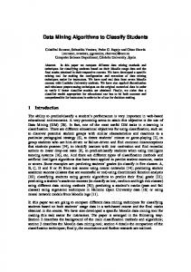
Figure 1: Class diagram of data mining algorithm’s blocks.

For the cycle for attributes, (i) initialization function 𝑓𝑏init𝐴 performs initialization of an attribute counter by initializing this counter with the use of index of the first attribute; (ii) conditional function 𝑐𝑓𝐴 checks whether all the attributes have been processed; (iii) preprocessing function 𝑓𝑏prev𝐴 changes an attribute counter assigning the index of the next vector. Thus, an attribute cycle can be determined as an embedded function of the highest order in the following form: loop 𝐴 ~ 𝐹𝐵; loop 𝐴 = loop’ (𝑑, 𝑓𝑏init𝐴(𝑑, 𝑚), 𝑓𝑏init𝐴, 𝑓𝑏pre𝐴, 𝑓𝑏iter ).

Next, consider the implementation of typed blocks with the unified interface and the pure function. These blocks are functional blocks.

4. Implementation of Functional Blocks We implemented all described new functional blocks as classes of an object-oriented language Java. Figure 1 shows the class diagram of blocks (units) of the data mining algorithm. Here the simple step (functional block) of the data mining algorithm is described by the class Step. The implementation step of the algorithm is contained in the method execute(). Calling of this methods leads to

6

Mathematical Problems in Engineering

(1) for each vector (2) build the transactions list from the data set; (3) end for each vector (4) for each transactions (5) for each item set from transactions (6) calculate support of 1-item sets (7) create large 1-item sets (8) end for each item set from transactions (9) end for each transactions (10) for each large 𝑘-item set list while list ≠ ⌀ (11) for each 𝑘 − 1-item set (12) for each 𝑘 − 1-item set starting with current (13) create 𝑘-item set candidate (14) if is candidate created then (15) for each transactions (16) calculate support of candidate (17) end for each transactions (18) remove candidate with small support (19) end for each 𝑘 − 1-item item set (20) end for each 𝑘 − 1-item item set (21) end each large 𝑘-item set list (22) for each large 𝑘-item set list while list ≠ ⌀ (23) for each large 𝑘-item set from list (24) for each item from large 𝑘-item set (25) create association rules (26) end for each item (27) end for each large 𝑘-item set (28) end each large 𝑘-item set list Algorithm 2: The algorithm Apriori.

execution of the step. This method returns mining model and has followed input arguments: (i) constructing mining model—model; (ii) data set—inputData. The method execute() is the basis method of step; therefore, it must be implemented as the pure function. For this, it works only with input arguments (model and inputData) and has not any references to other variables. For a data mining algorithm, it is typical to perform data processing by vectors and also by the values of each attribute. Since the decision and the cycle are the steps of the algorithm, classes corresponding to them are inherited from the class Step. The class DecisionStep corresponds to the decision and the class CyclicStep to the cycle. Both of these classes contain the necessary links to the data set (inputData) and the mining model (model). In addition, the class DecisionStep contains (i) sequence of steps which executed when the condition is true: trueBranch; (ii) sequence of steps which executed when the condition is false: falseBranch. The condition itself is defined in the method condition(). The class CyclicStep in addition to the methods and attributes of the class Step defines sequence of the steps that make up one iteration of a cycle—iteration. Initialization of

a cycle is defined in the method initLoop(). Condition of the cycle (loop) termination is implemented in the method conditionLoop(). In addition to these methods in the class CyclicStep defined methods to implement preprocessing before each iteration beforeIteration() and postprocessing after each iteration afterIteration(). For the implementation of cycle for vectors defined class VectorsCycleStep. It implements the necessary methods of the class CyclicStep, providing selection of vectors of a data set. Processing of each vector is determined by the sequence of steps added to the iteration—iteration. Similarly, for processing of values of attributes, the class AttributesCycleStep is implemented. The classes DecisionStep and CyclicStep use the class StepSequence to determine the sequences of steps. The sequence of steps in itself is a step of the algorithm; therefore, the class StepSequence is inherited from the class Step. The object of this class contains a set of objects of class Step corresponding to the steps of the algorithm and being executed sequentially one after another. To add a step to the sequence use method addStep(). To form the target algorithm define the class MiningAlgorithm. It contains a sequence of all steps of the algorithm— steps—and also methods: (i) initSteps()—initializing steps of the algorithm. (ii) runAlgorithm()—launching the algorithm. (iii) buildModel()—building the model.

Mathematical Problems in Engineering

7

(1) for each vector (2) build the transactions list from the data set; (3) end for each vector (4) for each transactions (5) for each item set from transactions (6) calculate support of 1-item sets (7) create large 1-item sets (8) for each item set from transactions starting with current (9) create the hash table for 2-item sets (10) end for each item set (11) end for each item set (12) end for each transaction (13) pruning the hash table (14) for each large 𝑘-item set list while list ≠ ⌀ (15) for each item set from (16) for each item set from starting with current (17) create k-item sets with the hash table (18) create the hash table for k + 1 item sets (19) if is candidate created then (20) for each transactions (21) calculate support of candidate (22) end for each transactions (23) remove candidate with small support (24) end for each item set (25) end for each item set (26) end each large 𝑘-item set list (27) pruning the hash table (28) for each large 𝑘-item set list while list ≠ ⌀ (29) for each large 𝑘-item set from list (30) for each item from large 𝑘-item set (31) create association rules (32) end for each item (33) end for each large 𝑘-item set (34) end each large 𝑘-item set list Algorithm 3: The algorithm DHP.

In essence in the method initSteps() occurs formation of algorithm structure by creating of the steps which determining of sequence and nesting of their execution. For possibility of parallel execution of parts of algorithm, the class StepSequence implements the interface java.lang.Runnable, determining thereby that the sequence of steps can be launched in a separate thread. What parts of the algorithm must be executed in separate sequences (and as a consequence in the subsequent will be executed in separate threads) is defined in the method initSteps() in the process of formation of the algorithm and corresponding objects of the class StepSequence.

5. Examples of Algorithm Building Now consider applying of the suggested method for a family of Apriori algorithms. In order to illustrate correctness and efficiency of the suggested approach, we will implement algorithms of one group on the basis of functional blocks described earlier. We will show that algorithm decomposition into functional blocks and implementation of these blocks using the suggested approach allows us to obtain new

modifications of algorithms by minor changes in program code. The Apriori algorithm [1] is described in 1994 by Agrawal and Srikant. In 1994 and 1995 modifications of this algorithm were suggested: (i) Apriori—the feature of this algorithm is that the database is not used for counting support after the first pass [1]. (ii) DHP—uses hash-table for reducing of the data set that handled after first iteration [2]. (iii) Partition—splits the data set on parts that have a size enough for an operation memory [3]. All algorithms are present in Algorithms 2, 3, 4, and 5. We implement functional blocks as Java classes for each of them. Figure 2 shows the class diagram of all functional blocks. In the lower part of the diagram, there are algorithm classes (successors of the class MiningAlgorithms) containing the sequence of functional block calls. The first algorithm to be implemented was Apriori TID together with all the necessary functional blocks.

8

Mathematical Problems in Engineering

(1) for each vector (2) build the transactions list from the data set and create TID list for item; (3) end for each vector (4) for each block of transaction list (5) split data set on parts (6) end for each block of transaction list (7) for each partition (8) for each transactions (9) for each item set from transactions (10) generate TID list for item set (11) create large 1-item sets (12) end for each item set from transactions (13) end for each transactions (14) for each large 𝑘-item set list while list ≠ ⌀ (15) for each 𝑘 − 1-item set (16) for each 𝑘 − 1-item set starting with current (17) create k-item sets with TID (18) remove candidate with small support (19) end for each item set (20) end for each transactions (21) end each large 𝑘-item set list (22) end for each partition (23) for each large 𝑘-item set list while list ≠ ⌀ (24) for each partition (25) for each large 𝑘-item set from list (26) for each item from large 𝑘-item set (27) creating association rules (28) end for each item (29) end for each large 𝑘-item set (30) end for each partition (31) end each large 𝑘-item set list Algorithm 4: The algorithm Partition.

The next algorithm to be implemented was algorithm DHP. As can be seen from the description, this algorithm is the modification of Apriori TID and it uses hash-tables for storing frequent sets (modifications are highlighted in bold). Algorithm implementation required us to add three new functional blocks and block calls, which have been included in the algorithm class (successor of MininigAlgorithm). We have also implemented Partition algorithm, which is another modification of Apriori TID algorithm and divides the whole dataset into parts for more rapid processing. Three new blocks were created for its implementation and the corresponding changes have been made in the algorithm class. Using existing functional blocks we easily can create new data mining algorithm. It will have features of algorithms Apriori TID, DHP, and Partition. Algorithm 4 shows this algorithm. At the same time it was not necessary to implement new functional blocks. The corresponding changes have been made only to the algorithm class (successors of the class MiningAlgorithms). Table 1 shows changes made in the code of the described algorithms. Changes are shown in evaluation code lines (metric ELOC). Implementation of all the algorithms was performed in Java. The implemented algorithms were tested on similar test datasets. The results obtained after testing

coincide with reference ones, which confirms implementation correctness in the case when the algorithms are sets of functional blocks. Thus, software implementation on the basis of the AprioriTID algorithm required as follows: (i) DHP required us to change/add 22% of code. (ii) Partition required us to change/add 17% of code. (iii) Combined algorithm required us to change/add 2% of code. This is significantly lower than the creation of the algorithms from the very beginning. Furthermore, in order to construct the algorithms, debugged functional blocks are used, which reduces the time and effort for algorithm debugging.

6. Conclusion The present paper discusses the model of data mining algorithm representation in a functional way. This model is an extension of 𝜆-calculus and retains its principles. The model includes new types for dataset definition, mining models, and also a number of functions. Furthermore, new functions have been added in accordance with the main elements of data mining algorithms.

Mathematical Problems in Engineering

9

(1) for each vector (2) build the transactions list from the data set and create TID list for item; (3) end for each vector (4) for each block of transaction list (5) split data set on parts (6) end for each block of transaction list (7) for each partition (8) for each transactions (9) for each item set from transactions (10) generate TID list for item set (11) creating large 1-item sets (12) for each item set from transactions starting with current (13) creating the hash table for 2-item sets (14) end for each item set (15) end for each item set from transactions (16) end for each transactions (17) pruning the hash table (18) for each large 𝑘-item set list while list ≠ ⌀ (19) for each 𝑘 − 1-item set (20) for each 𝑘 − 1-item set starting with current (21) create k-item sets with TID and the hash table (22) create the hash table for k + 1 item sets (32) remove candidate with small support (23) end for each item set from transactions (24) end for each item set from transactions (25) end each large 𝑘-item set list (26) pruning the hash table (27) end for each partition (28) for each large 𝑘-item set list while list ≠ ⌀ (29) for each partition (30) for each large 𝑘-item set from list (31) for each item from large 𝑘-item set (32) creating association rules (33) end for each item (34) end for each large 𝑘-item set (35) end for each partition (36) end each large 𝑘-item set list Algorithm 5: The algorithm as combination of algorithms Apriori TID, DHP, and Partition.

Table 1: Values of changes included in code. Metrics\algorithms

Apriori TID DHP Basis classes (successors of class MiningAlgorithms) ELOC of changes for basis class 71 79 Changes in comparison with Apriori TID 0 8 Functional blocks (successors of class Step) Number of blocks 15 18 Added blocks 15 3 ELOC for additional blocks 329 124 Total number of ELOC 400 603 Changes, % 0 22

As a result, the functional model of a data mining algorithm presents the algorithm as a set of embedded unified pure functions (functional blocks). This makes it possible to modify algorithms due to block switching and block substitution. It also helps reduce the time and effort needed

Partition

Combination

81 10

90 19

18 3 86 567 17

21 0 0 770 2

for data mining algorithm modification and creation of new algorithms. The paper also contains description of software implementation of a functional model as a set of Java classes. These classes were used for implementing algorithms from

10

Mathematical Problems in Engineering apriori.steps.GenerateAssosiationRuleStep

apriori.steps.RemoveUnsupportItemSetStep

apriori.partition.steps.GenerationTIDListStep

apriori.steps.IsThereCurrenttCandidate

apriori.steps.LargeItemSetItemsCycleStep

apriori.steps.CreateLarge1ItemSetStep

apriori.steps.TransactionItemsCycleStep

apriori.steps.BuildTransactionStep DecisionStep

apriori.steps.KLargeItemSetsCycleStep apriori.partition.steps.BuildTIDTransactionStep CycleStep

apriori.steps.Calculate1ItemSetSupportStep

apriori.steps.K_1LargeItemSetsCycleStep

apriori.steps.TransactionItemSetsCycleStep apriori.dhp.steps.CreateHashTableStep

Step apriori.steps.K_1LargeItemSetsFromCurrentCycleStep

apriori.steps.CalculateKItemSetSupportStep apriori.steps.LargeItemSetListsCycleStep apriori.dhp.steps.CreateLargeItemSetsWithHashTableStep

apriori.steps.CreateKItemSetCandidateStep

apriori.partition.steps.CreateKItemSetCandidateWithTIDsStep

apriori.dhp.steps.HashTablePruningStep

org.eltech.ddm.miningcore.algorithms.MiningAlgorithm

apriori.AprioriAlgorithm

apriori.partition.PartitionAlgorithm

apriori.dhp.DHPAlgorithm

Figure 2: Classes for algorithms Apriori TID, DHP, and Partition.

the Apriori family: Apriori TID, DHP, and Partition. Implementation of these algorithms was performed by adding several classes and changing several lines. Furthermore, combination of existing functional blocks allowed us to obtain an algorithm that has all the properties of the algorithms listed above. Further research will be conducted in the area of algorithm parallelization. We plan to explore possibilities of data mining algorithm parallelization when the algorithms consist of functional blocks. Parallelization will be based on both data and tasks. Solution of this task will allow us to dramatically reduce time and effort for converting a sequential algorithm into a parallel one.

Conflict of Interests The authors declare that there is no conflict of interests regarding the publication of this paper.

Acknowledgments The paper has been prepared within the scope of the state project “Organization of scientific research” of the main part

of the state plan of the Board of Education of Russia as well as the project part of the state plan of the Board of Education of Russia (Task no. 2.136.2014/K).

References [1] R. Agrawal and R. Srikant, “Fast algorithms for mining association rules in large databases,” in Proceedings of the 20th International Conference on Very Large Data Bases (VLDB ’94), pp. 487–499, Santiago, Chile, 1994. [2] J. S. Park, M.-S. Chen, and P. S. Yu, “Using a hash-based method with transaction trimming for mining association rules,” IEEE Transactions on Knowledge and Data Engineering, vol. 9, no. 5, pp. 813–825, 1997. [3] A. Savasere, E. Omiecinskia, and S. Navathe, “An efficient algorithm for mining association rules in large databases,” in Proceedings of the 21th International Conference on Very Large Data Bases (VLDB ’95), pp. 432–444, Zurich, Switzerland, 1995. [4] D. Knuth, The Art of Computer Programming, vol. 1-4A, Addison-Wesley Professional, 2011. [5] T. H. Cormen, C. E. Leiserson, R. Rivest, and C. Stein, Introduction to Algorithms, MIT Press, Cambridge, Mass, USA, 3rd edition, 2009.

Mathematical Problems in Engineering [6] G. M. Amdahl, “Validity of the single processor approach to achieving large scale computing capabilities,” in Proceedings of the Spring Joint Computer Conference (AFIPS ’67), vol. 30, pp. 483–485, Thompson Books, Washington, DC, USA, April 1967. [7] J. L. Peterson, Petri net theory and the modeling of systems, Prentice-Hall, Englewood Cliffs, NJ, USA, 1981. [8] T. Murata, “Petri nets: properties, analysis and applications,” Proceedings of the IEEE, vol. 77, no. 4, pp. 541–580, 1989. [9] Vl. V. Voevodin and V. V. Voevodin, “Analytical methods and software tools for enhancing scalability of parallel applications,” in Proceedings of the Intelligent Conference on HiPer, pp. 489– 493, 1999. [10] Haskell programming language, http://www.haskell.org/. [11] Common Lisp Language, https://common-lisp.net/. [12] N. Kerdprasop and K. Kerdprasop, “Mining frequent patterns with functional programming,” International Journal of Computer, Information, Systems and Control Engineering, vol. 1, no. 1, pp. 120–125, 2007. [13] L. Allison, “Models for machine learning and data mining in functional programming,” Journal of Functional Programming, vol. 15, no. 1, pp. 15–32, 2005. [14] O. Maimon and L. Rokach, Decomposition Methodology for Knowledge Discovery and Data Mining: Theory and Applications, Machine Perception and Artificial Intelligence, World Scientific, 2005. [15] T. G. Dietterich, “Ensemble methods in machine learning,” in Proceedings of the 1st InternationalWorkshop on Multiple Classifier Systems, pp. 1–15, Springer, Berlin, Germany, 2000. [16] L. Todorovski and S. Dˇzeroski, “Combining multiple models with meta decision trees,” in Principles of Data Mining and Knowledge Discovery, vol. 1910 of Lecture Notes in Computer Science, pp. 54–64, Springer, Berlin, Germany, 2000. [17] RapidMiner, http://rapidminer.com/. [18] P. M. Gonc¸alves Jr., R. S. M. Barros, and D. C. L. Vieira, “On the use of data mining tools for data preparation in classification problems,” in Proceedings of the IEEE/ACIS 11th International Conference on Computer and Information Science (ICIS ’12), pp. 173–178, IEEE, Shanghai, China, June 2012. [19] Waikato Environment for Knowledge Analysis (Weka), http://www.cs.waikato.ac.nz/ml/weka/. [20] I. H. Witten, E. Frank, L. Trigg, M. Hall, G. Holmes, and S. J. Cunningham, “Weka: practical machine learning tools and techniques with java implementations,” in Proceedings of the Workshop on Emerging Knowledge Engineering and Connectionist-Based Information Systems (ICONIP/ANZIIS/ ANNES ’99), pp. 192–196, 1999. [21] R language, http://www.r-project.org/. [22] S. Tippmann, “Programming tools: adventures with R,” Nature, vol. 517, no. 7532, pp. 109–110, 2014. [23] F. Morandat, B. Hill, L. Osvald, and J. Vitek, “Evaluating the design of the R language: objects and functions for data analysis,” in Proceedings of the 26th European Conference on Object-Oriented Programming (ECOOP ’12), J. Noble, Ed., pp. 104–131, Springer, Beijing, China, June 2012. [24] A. Ghoting, P. Kambadur, E. Pednault, and R. Kannan, “NIMBLE: a toolkit for the implementation of parallel data mining and machine learning algorithms on mapReduce,” in Proceedings of the 17th ACM SIGKDD International Conference on Knowledge Discovery and Data Mining (KDD ’11), pp. 334–342, San Diego, Calif, USA, August 2011.

11 [25] H. P. Barendregt, The Lambda Calculus: Its Syntax and Semantics, vol. 103 of Studies in Logic and the Foundations of Mathematics, North-Holland, 1985. [26] A. Church and J. B. Rosser, “Some properties of conversion,” Transactions of the American Mathematical Society, vol. 39, no. 3, pp. 472–482, 1936. [27] F. Joachimski, “Confluence of the coinductive 𝜆-calculus,” Theoretical Computer Science, vol. 311, no. 1–3, pp. 105–119, 2004. [28] Common Warehouse Metamodel (CWM) Specification, OMG, Version 1.1, 2003, http://www.omg.org/cwm/.

Advances in

Operations Research Hindawi Publishing Corporation http://www.hindawi.com

Volume 2014

Advances in

Decision Sciences Hindawi Publishing Corporation http://www.hindawi.com

Volume 2014

Journal of

Applied Mathematics

Algebra

Hindawi Publishing Corporation http://www.hindawi.com

Hindawi Publishing Corporation http://www.hindawi.com

Volume 2014

Journal of

Probability and Statistics Volume 2014

The Scientific World Journal Hindawi Publishing Corporation http://www.hindawi.com

Hindawi Publishing Corporation http://www.hindawi.com

Volume 2014

International Journal of

Differential Equations Hindawi Publishing Corporation http://www.hindawi.com

Volume 2014

Volume 2014

Submit your manuscripts at http://www.hindawi.com International Journal of

Advances in

Combinatorics Hindawi Publishing Corporation http://www.hindawi.com

Mathematical Physics Hindawi Publishing Corporation http://www.hindawi.com

Volume 2014

Journal of

Complex Analysis Hindawi Publishing Corporation http://www.hindawi.com

Volume 2014

International Journal of Mathematics and Mathematical Sciences

Mathematical Problems in Engineering

Journal of

Mathematics Hindawi Publishing Corporation http://www.hindawi.com

Volume 2014

Hindawi Publishing Corporation http://www.hindawi.com

Volume 2014

Volume 2014

Hindawi Publishing Corporation http://www.hindawi.com

Volume 2014

Discrete Mathematics

Journal of

Volume 2014

Hindawi Publishing Corporation http://www.hindawi.com

Discrete Dynamics in Nature and Society

Journal of

Function Spaces Hindawi Publishing Corporation http://www.hindawi.com

Abstract and Applied Analysis

Volume 2014

Hindawi Publishing Corporation http://www.hindawi.com

Volume 2014

Hindawi Publishing Corporation http://www.hindawi.com

Volume 2014

International Journal of

Journal of

Stochastic Analysis

Optimization

Hindawi Publishing Corporation http://www.hindawi.com

Hindawi Publishing Corporation http://www.hindawi.com

Volume 2014

Volume 2014