Decoupled illumination detection in light sheet microscopy for fast volumetric imaging: supplementary material OMAR E. OLARTE,1 JORDI ANDILLA,1 DAVID ARTIGAS1,2 AND PABLO LOZAALVAREZ1,* 1ICFO-Institut
de Ciencies Fotoniques, Av.Carl Friedrich Gauss, 3, 08860 Castelldefels (Barcelona), Spain of Signal Theory and Communications, Universitat Politècnica de Catalunya, Jordi Girona 1-3,08034 Barcelona, Spain *Corresponding author:
[email protected] 2Department
Published 04 August 2015
This document provides supplementary material to "Decoupled illumination detection microscopy in light sheet microscopy for fast volumetric imaging,” http://dx.doi.org/101364/optica.2.000702. Current microscopy demands for the visualization of large three-dimensional samples, with increased sensitivity, higher resolutions and faster speeds. Several imaging techniques based on widefield, point-scanning and light-sheet strategies have been designed to tackle some of these demands. Although successful, all these possess an important requirement: The illuminated volumes need to be tightly coupled with the detection optics to accomplish efficient optical sectioning. Here we break this paradigm and produce optical sections from out of focus planes. This is done by extending the depth-of-field of the detection optics in a light-sheet microscope, using wavefront coding techniques. This passive technique allows freely accommodating the light sheet to any place within the extended axial range. We show that this enables quickly scanning the light-sheet across a volumetric sample. In consequence imaging speeds faster than twice volumetric video-rate (>70 volumes/s) can be achieved without the need of moving the sample. These capabilities are demonstrated for volumetric imaging of fast dynamics in vivo as well as for fast three-dimensional particle tracking. In this supplementary material we present: a detailed materials and methods section and a detailed characterization of the system. © 2015 Optical Society of America http://dx.doi.org/10.1364/optica.2.000702.s001
1. MATERIALS AND METHODS DID-LSFM optical setup
The current optical setup of DID-LSFM is shown in Fig. S1. The detailed description and characterization of the base LSFM optical setup can be found in Olarte et al. [1]. The optical components employed are listed in Table S2. In the base LSFM setup several different light-sheet modalities coexist in the excitation path: selective plane illumination microscopy (SPIM, i.e., based on the use of a cylindrical lens) and one- and two-photon Digital Scanned Light Sheet Microscopy (DSLM) with either Gaussian or Bessel beams can be selected. For this work we only employed SPIM and linear DSLM with Gaussian beams excitation modalities (see Fig. S1). We have employed a diode laser (λ=488nm, 50mW) as excitation source, keeping the laser power at the sample plane
below 0.5mW. A galvanometric mirror (GM) is used for the axial scanning of the light-sheet. The generated fluorescence is collected with a water dipping infinity-corrected objective (CO), located in the collection arm of the LSFM. An optical system, composed by a couple of steering mirrors, MF1 and M, and a couple of relay lenses, L3 and L4, is used to conjugate the exit pupil of the CO to the surface of a deformable mirror (DM). The DM (Mirao52e™, Imagine Optic) generates the phase map required for extending the DOF of the CO. A Shack-Hartmann wavefront sensor (WFS, HASO v3™, Imagine Optic) is employed to ensure proper shape of the DM. The DM is placed at a conjugated plane to the wavefront sensor using a couple of relay lenses, L5 and L6, and two additional steering mirrors, MF2 and MF3. A proprietary software (CASAO™, Imagine optic) is used to properly shape the DM according to the optical wavefront measured with the WFS. MF3 is removed from
2
the optical path once the DM has the correct shape. Finally, lens L5 is effectively employed as a tube lens that focuses the captured fluorescent light on the sCMOS detector. MF1, MF2 can be moved to enable/disable the WFC optical path, allowing the optical setup to be used as a regular LSFM.
aberration present on the imaging system is intrinsically corrected due to the deconvolution process. In terms of sample aberrations, these can be corrected using several adaptive optics strategies. In our setup this can be done by adding an previously measured phase correction to the generated WFC phase mask [2]. Cubic phase mask (CPM) generation
Fig. S1. Lay out of the optical setup.
Table S1. Detailed list of the optical elements. Item Manufacturer/model Notes Laser Cobolt MLD/ 0488-06488nm , 010060-100 150mW Galvo Mirrosr/GM Thorlabs/GVS002 L1 Thorlabs/LA1027-A F=35mm L2 Thorlabs/LA1433-A F=150mm Excitation objective/EO Nikon/Plan Fluor 10x NA=0.3, WD=16mm Sample holder/SH Thorlabs/3-axis Stepper NanoMax, Physik motors for instrumente Mxyz 116.2SH translation and ϕ rotation. Collection objective CO Leica/HCX apo L20X NA=0.5 L3 Thorlabs/AC254-200F=200mm A Poc Collection objective Square, pupil 10mm side L4 Thorlabs/AC254-250F=250mm A DM-Deformable Mirror Imagine optic/Mirao52e L5 Thorlabs/AC508-250F=250mm A L6 Thorlabs/AC254-060F=60mm A WFS Imagine optic/Haso 3 32 Detector Hamamatsu/ ORCAFlash 4.0 C11440-22C Synchronization/Control National instruments/PCIe6353
Note that this set up has the advantage that it can also be used to compensate aberrations in a straightforward manner. Any
The Cubic phase masks (CPMs) were generated in a DM using a closed-loop approach that iteratively sets and corrects the shape of the DM according to the specified wavefront targets using a WFS. The final mirror shapes, for each CPM and the flat reference, were digitally stored once the difference between the target and the generated wavefronts was less than 30 nm RMS. As we use a WFS it is convenient to express the strength, α, of the masks in wavefront peak-to-valley amplitudes, WPV. Conversion between the two parameters can be found in Section 2. To target DOFs of ~200 μm, large enough for most of LSFM experiments, CPMs with α ≈ 65 is required (see Section 2). We have therefore designed two CPMs around the optimal α value with WPV = 10 and 20 μm (α = 40 and 80). A WPV = 30 μm (α = 120) was also used to test the DM at the limit of its dynamic range. The mask design was done using proprietary software (HASOv3™). Fluorescent beads of 1 μm in diameter, sparsely embedded in agar, were used as illumination point sources to perform the wavefront measurements required to set the shape of the DM. To select one single bead, the light sheet amplitude (in a DSLM configuration) was set to minimum and the sample was translated until a single bead was found in the center of the FOV. Calibration
To account for the z-dependent shift introduced by the cubic phase mask (CPM), a sample of sparsely distributed fluorescent microbeads suspended in AGAR was prepared (see: Sample preparation and mounting). The same volume in the sample was imaged with both, the standard LSFM and the DID-LSFM systems. The standard LSFM volumetric image was used as a ground-truth reference. To calculate the space transformation between them, the (x, z) and (y, z) positions of the microspheres in both sets of data were found by calculating their centroids. Then, twenty-five matching point pairs were selected from both data sets, and loaded into our transformation algorithm. To properly model the quadratic shift of the CPM a second-order polynomial transformation was used. Once the transformation (and its inverse) was calculated this was used to correct for the zdependent shift in all our LSFM-DID datasets. Finally, as our standard LSFM image was used as a ground-truth reference, the transformation also compensated any other image distortion present in a DID-LSFM image. Deconvolution, OTF, and particle tracking
Deconvolution was performed using the Richardson-Lucy (RL) algorithm [3] which is an iterative expectation maximization algorithm based on a Bayesian framework. The RL algorithm converges to the maximum likelihood solution for Poisson statistics [4]. This is a suitable statistical model describing the emission and detection of photons in LSFM [5]. One of the main advantages of RL deconvolution is that the restored images are robust against small errors in the point-spread function (PSF) and therefore, very convenient for WFC imaging. Here, a basic version of the algorithm was used. In this, no image priors have been introduced and therefore no regularization terms were used. The only free parameter was the number of allowed iterations. We found that typically 20 iterations were enough to
3
restore the images. Under such conditions, our algorithm took 1 second per iteration for full-frame images. The required PSFs for deconvolution were obtained from beads immersed in agar. Single PSFs were cropped making sure that no other PSF (in neighbor planes or regions) were present and making sure that the cropping area was much bigger than the total extension of the PSF. The PSF was then background-corrected, resized and centered before loading them to the deconvolution routine. PSF was obtained for every plane allowing a plane-byplane deconvolution. OTF profiles were calculated by Fourier transforming the intensity PSFs. Fourier transforms were computed using the Fast Fourier Transform. Once the OTFs are calculated, the cut-off frequency for each case is found to determine the final resolution of the system (see Section 3). Particle tracking was manually performed before applying the deconvolution procedure. Basically, the main lobe of each PSF is manually selected by defining a ROI (~ 10pixels2) around it at the plane of maximum intensity. Then the lobe within this ROI was fitted to a 3D Gaussian function (GF) assigning its 3D coordinates to its center. Afterwards the space transformation to correct the quadratic shift in the PSF was performed. Manual tracking before deconvolution was chosen because it allowed tracking particles that were at the extremes of the FOV where the full PSF information was not available.
the chamber from a hole machined at one face of the cube, the objective is held with the chamber with an o-ring that prevents any fluid leaking. Fluorescent microspheres
We employed green fluorescent microspheres of 0.2 and 1 μm (Duke scientific, G200 and G0100, 2% solids) for the experiments reported in this work. To obtain a sample of microspheres sparsely distributed over the imaging volume we prepared a dilution 1:1000 in ultrapure water (type 1, Milli-Q,). Different aliquotas of this stock solution were stored in 1.5 ml conical tubes. The stock solution were vortexed for 30 s before preparing the sample for imaging to obtain a disperse distribution. We added 10 μl of the stock solution to 0.1 ml of 1% low-melting agarose (LMA) at 45oC in another 1.5 ml conical tube and vortex gently. Agarosemicrobead solution were drawn directly to a glass capillary (Hirschmann Z611263, 100 μl) with a micropipette. Samples were incubated at 4oC for 5 min for stabilization and then mounted into a custom made LSFM sample holder. A custom-made plunger was used to force the agar cylinder out of the capillary in front of the detection objective. For the particle tracking experiments, a sample 0.2 μm microspheres was prepared. Just before the experiment the agar cylinder was forced to rapidly get out the capillary releasing some microspheres in the medium just on top of the FOV of the microscope. Experiment started within 20 s after releasing the microspheres.
Control software
A custom made Labview™ interface was specifically developed to operate and synchronize the acquisition of the microscope images with the GM scanning system. Two acquisition modes were used: i) External controlled mode (synchronous) and ii) free running mode (asynchronous). In the synchronous mode, the GMs are driven by a triangle and saw-tooth voltage signals for fast (y axis, in case DSLM mode is used) and slow (z axis) mirrors, respectively. A step-function trigger-signal controls the data acquisition of the camera and ensures that every image is taken when the GMs are static. All these voltage signals were generated by a NI USB-6353 data acquisition and generation device (National Instruments Corp., Austin, TX, USA). The z-scanning signal was generated in steps per image. For each z position, a trigger signal is fired just after the GM reaches the programmed value and an image is captured. The exposure time was set to a value slightly lower than the step interval. The maximum frame rate practically achievable with this synchronous configuration is 250fps as this corresponded to an integration time of just over 1ms, the minimum allowed by the sCMOS in the actual configuration. In the free running mode the GM are also driven by a triangle and saw-tooth voltage as before but in this case, there is no triggering signal controlling the acquisition of the camera. In this mode, the camera continuously acquires images at the specified frame rate. This allows taking advantage of the maximum integration time of the camera for modes faster than 250fps. Sample preparation and mounting
The samples are held by a custom made capillary sample holder (SH) that is attached to a three axis motorized stage (x, y and z) and a rotation stage that controls the angle ø. The SH is located into a custom-made immersion chamber that is filled with a physiological fluid (PBS) that keeps the samples in osmotic equilibrium. Chamber is made from a cube of PTFE (Teflon) optically accessible from three glass windows made with coverslips (N= 1.5, 170 μm thickness). The objective lens enters
C. elegans samples
C. elegans were grown on nematode growth medium agar plates using standard procedures [6]. We employed two transgenic strains for this work, first; the ljIs1[myo2::YC2.1] line showing expression of yellow cameleon2.1 (YC2.1) throughout the pharynx and, second, the juIs76[unc25::GFP] line expressing GFP in a subset of D-type moto-neurons. Adult hermaphrodite worms were immobilized into a 5 μl drop of sodium azide (NaN3, 25 mM) for 10 minutes. A few worms were then picked and transferred to a 5 μl drop of PBS. Then, a micropipette tip (0.1 ml) was loaded with 50 μl of LMA (1%, 45oC) keeping the plunger temporarily depressed in order to draw the drop containing the worms into the micropipette tip by a slow releasing of the plunger. Immediately after, the agar-worm solution was drawn directly from the tip into a glass capillary using the micropippeter. This transfer was done slowly so as to keep the worms evenly distributed in the agar cylinder. Samples were then incubated at 4oC for 5 min for stabilization (and for further immobilization) and then mounted into a custom made LSFM sample holder. A custom made plunger was used to force the agar cylinder out of the capillary in front of the detection objective.
2. WAVEFRONT CODING (WFC) WFC extends the DOF of an imaging system by modifying its Optical Transfer Function (OTF). This is done by modifying the pupil of the imaging lens, normally by the use of a cubic phase masks (CPM) according to a phase function of the form φ(u) = α (ux3 + uy3), where ux,y are the coordinates on the normalized space of spatial frequencies of a square pupil. Note that u=f/2f0, where f are the spatial frequencies and 2f0 is the incoherent frequency-limit given by diffraction. For our system 2f0 = 1340 cycles/mm. This function depends on a single parameter α that represents the amplitude of the phase modulation. The third order dependence was found by minimizing the variation of the modulus of the OTF (MTF) with the defocus term, ψ, by using a stationary phase approximation [7]. By doing
4
so, the MTF is approximately invariant except for a phase component given by ψ2/3α. This phase factor gives rise to a translation (z-dependent shift) as well as an additional phase component that results in an additional phase modulation and therefore in imaging artifacts [8]. For the implementation of the CPM using the DM, the desired phase change was generated according to the required α. The phase change induced by the DM was monitored using a Shack-Hartmann sensor that reports the peak-to-valley (WPV) values of the wavefront aberrations. For a square pupil, α is related with the WPV as, α = 0.25kWPV, where k = 2π/λ is the wavenumber of the fluorescence. Fig. S2 shows the theoretically calculated three-dimensional PSF and three experimentally measured PSFs along the z axis. Both of the described effects, the z-related shift and the change of the structure of the PSF at the extremes of the DOF are evident from these figures.
used for deconvolving a volumetric image. This is not a problem in our DID approach as the PSF can be measured at each z-position (plane) and each of these is used for deconvolving each of the respective planes.
Fig. S3. Size variation of the PSFs as measured for CPMs with different α parameter. The average size and standard deviation of the different PSFs was determined by measuring line profiles along x and y directions for 5 different beads
Fig. S2. Three-dimensional PSF of WFC for α = 40. The left hand side panel corresponds to the xz-view of the PSF obtained numerically for an axial range of 200 μm around the center of the DOF. The quadratic z-dependent shift on the PSF can be observed. The images on the central and right columns show the calculated and experimental xy PSFs at z = -85, 0 and 85 μm. Scale bar 20 μm
3. RESOLUTION IN DID-LSFM DID-LSFM properties for different α values.
By using microbeads (see Section 1), we measured the PSFs across the imaged volume for the three CPMs employed in this work (α = 40, 80 and 120). For each z position, the average size and standard deviation of the different PSFs was determined by measuring line profiles along x and y directions for 5 different beads. The results as a function of z are shown in Fig. S3, where the size of the PSF has been normalized with respect to the size at the center of the DOF. To ensure that the relevant signal is considered an empirical intensity threshold of 0.05 × Imax was chosen (where Imax is the maximum intensity of the PSF). As can be appreciated, the PSFs are not perfectly invariant with defocus. It is, however, interesting to emphasize that the change in the relative size of the PSF (along the z axis) is smaller for higher α values. Such variation also suggests that there is a change in the xy resolution. Therefore, care has to be taken in standard WFC, since a unique PSF can be
Fig. S4. MTFs showing the contained frequencies of the DID-LSFM at the center of the DOF for different CPMs having α values of 40 (green), 80 (blue) and 120 (red). For comparison, the black lines (dotted and continuous) are, respectively, the theoretical and measured MTF for a standard light sheet microscope (i.e. α = 0). The color dotted lines represent the noise level (inverse of the SNR). Arrows show the maximum frequency, um, supported by the system for each of the CPM. These are: α = 40, um = 0.95; for α = 80, um = 0.82 and for α = 120, um = 0.70. From these values, a maximum loss (relative to α = 0) of up to 30 % of the contained frequencies is obtained when α = 120. Note that u = f/2f0, where f are the spatial frequencies and 2f0 is the incoherent frequency-limit given by diffraction. For our system 2f0 = 1340 cyc/mm.
Having a PSF for each of the different z planes allows for performing a proper and accurate quantification of the resolution change with defocus. To do that, we obtained from the PSFs, the experimental optical transfer function (OTF) of the DID-LSFM
5
system (see Section 1) for the three different CPMs. Fig. S4 shows the experimental modulus of the OTF (MTF) for the three CPMs, at the center of the DOF. For comparison purposes the theoretical and measured MTF for our microscope in a standard light sheet configuration (i.e. α = 0) is also shown. The dotted horizontal lines correspond to the noise level (inverse of the SNR) for each case. The intersection of these lines with the MTFs determines the maximum frequency, um (shown by arrows), supported by the system for a given SNR, and therefore, determines the maximum resolution. As expected, the use of WFC reduces the extent of the MTF (resolution) in all of the studied cases at the center of the DOF (up to a maximum of 25 % for α = 120). Finally, note that deconvolution should be performed to the images taken with our DID system. This process, although increasing the contrast of high frequencies, does not increase the final resolution as this will still be determined by the maximum frequency, um, for each case. Any amplified signal above this level may show up as an artifact on the final image and should be discarded.
therefore, the maximum supported frequency um. This is illustrated in Fig. S6, where we show the variation of the MTF for different integration times. Similarly to fast imaging, other conditions may also result on a decreased SNR as shown in Fig. S6. These include scattering or weakly fluorescent samples. In those cases, a similar response is expected. Under such conditions, any recovery algorithm will be directly affected by a low SNR (for a complete analysis and comparison on the effect of SNR on the use of deconvolution algorithms see Ref [9]). As commented above, to avoid artifacts, any signal above the cut-off frequency should not be considered.
Fig. S6. Resolution of the DID-LSFM system having a CPM with an α = 40 at different integration times. Arrows show the maximum supported frequency um . These are as follows um = 0.94 at 2Hz; um = 0.75 at 50Hz; um = 0.4 at 250 Hz and um = 0.25 at 400 Hz. Dashed lines shows the noise level (inverse of the SNR)
Fig. S5. Maximum supported frequencies, um, along a scanned axial range of 170 µm for α values of 40 (green) 80 (blue) and 120 (red). From these data, a maximum variation in resolution (up to 30%, from um = 0.94 to um = 0.64) when α = 40 can be observed. The resolution is, however, more constant along the axial scanned range (less than 10% variation) when larger α values are used. (um = 0.76 for α = 80 and um = 0.67 for α = 120). The measurements were performed using the average MTF obtained for the different z positions.
To assess the change of resolution along a scanned axial range of 170 µm, the maximum frequency, um, was measured for several axial positions. Fig. S5 shows this variation in resolution for the different CPMs. As can be seen, the relative change in resolution for a given mask is larger for smaller α values. For example, for α = 40, there is a considerable change in um (resolution) along the measured axial range, from 0.64 at the extremes to 0.94 at the center. In contrast there is a negligible variation in um for the same axial range for α = 80 or 120. This indicates that, for these α values, the resolution remains almost constant through the axial range (um = 0.76 for α = 80 and um = 0.67 for α = 120). DID-LSFM for different SNR.
To assess the response of the DID-LSFM system (having a CPM with α = 40) under fast imaging conditions we increased the reading speed of the camera while keeping the illumination conditions constant. This effectively resulted in a decrease of the SNR that directly affects the high frequencies of the image and
4. CAMERA SPECIFICATIONS Under external control mode we obtained images at 2, 50, 100 and 250 Hz, whereas on the free running mode at 250, 400, 570 and 1600Hz. Table S2. Hamamatsu Orca flash 4.0, frame rates, pixel resolution and data transfer rates Mode (2048 × Y ) Free running mode External control mode pixels2 Data Data Frame Frame transfer transfer Y rate rate rate rate (pixels) (Hz) (Hz) (MB/s) (MB/s) 2048 100 840 90 755 1024 200 840 164 688 512 401 840 278 583 256 802 840 425 446 128 1603 840 579 304
6
Media Captions Visualization 1: Fast single particle tracking using DID-LSFM Tracked trajectories of the Brownian motion of microspheres (0.2 μm) freely floating in a saline buffer. Imaging was performed using the scattered light from the microspheres. The camera was set to the maximum capture speed available 1600 planes/s (Δτ= ms). 22 planes per volume were imaged, resulting in an imaging speed of 73 volumes per second. For this movie a CPM with α = 40 was employed. Tracking was performed on the raw data (without deconvolution). Time stamp and volume dimensions are shown on the movie. Axis units in μm. Visualization 2: In vivo fast volumetric imaging using DID-LSFM, projections. 3D, orthogonal views of a moving worm obtained with DID-LSFM after deconvolution. The imaging speed of the camera was set to 400 planes/s (Δτ = 2.2 ms). 50 planes per volume were imaged, resulting in an imaging speed of 8 volumes/s. For this movie a CPM with α = 80 was employed. Time stamp is shown on the movie. Scale bar 25 μm. Visualization 3: In vivo fast volumetric imaging using DID-LSFM, Rendering. 3D rendering corresponding to Visualization 2.
Visualization 4: In vivo fast volumetric imaging using DID-LSFM, volumetric videorate. 3D, orthogonal views of a moving worm obtained with DID-LSFM after deconvolution. The imaging speed of the camera was set to 576 planes/s (Δτ = 1.7 ms). 24 planes per volume were imaged, resulting in an imaging speed of 24 volumes/s (volumetric videorate). For this movie a CPM with α = 80 was employed. Time stamp is shown on the movie. Scale bar 25 μm. Visualization 5: DID-LSFM for in vivo fast particle tracking. 3D movements of larvae inside an endotokia matricida C. elegans. Left: Maximum intensity projection of larvae moving after deconvolution. Right: the corresponding color-coded depth map. The imaging speed of the camera was set to 100 planes/s (Δτ = 7 ms). 10 planes per volume were imaged, resulting in an imaging speed of 10 volumes/s. For this movie a CPM with α = 40 was employed. The characteristic L-shape obtained due to deconvolution is also present (the image has been rotated by about 10° for a better visualization). Time stamp and scale bar (10 μm) are shown on the movie.
References 1. O. E. Olarte, J. Licea-Rodriguez, J. A. Palero, E. J. Gualda, D. Artigas, J. Mayer, J. Swoger, J. Sharpe, I. Rocha-Mendoza, R. Rangel-Rojo, and P. LozaAlvarez, "Image formation by linear and nonlinear digital scanned lightsheet fluorescence microscopy with Gaussian and Bessel beam profiles," Biomed. Opt. Express 3, 1492–1505 (2012). 2. R. Jorand, G. Le Corre, J. Andilla, A. Maandhui, C. Frongia, V. Lobjois, B. Ducommun, and C. Lorenzo, "Deep and Clear Optical Imaging of Thick Inhomogeneous Samples," PLoS ONE 7, e35795 (2012). 3. M. Laasmaa, M. Vendelin, and P. Peterson, "Application of Regularized Richardson-Lucy Algorithm for Deconvolution of Confocal Microscopy Images," Biophys. J. 100, 139a (2011). 4. L. A. Shepp and Y. Vardi, "Maximum likelihood reconstruction for emission tomography," IEEE Trans. Med. Imaging 1, 113–122 (1982). 5. E. G. Reynaud, U. Kržič, K. Greger, and E. H. K. Stelzer, "Light sheet-based fluorescence microscopy: More dimensions, more photons, and less photodamage," HFSP J. 2, 266–275 (2008).
6. T. Stiernagle, "Maintenance of C. elegans," in Wormbook, The C. elegans Research Community, ed. (2006). 7. J. Dowski and W. T. Cathey, "Extended depth of field through wave-front coding," Appl. Opt. 34, 1859–1866 (1995). 8. M. Demenikov and A. R. Harvey, "Image artifacts in hybrid imaging systems with a cubic phase mask," Opt. Express 18, 8207–8212 (2010). 9. T. Vettenburg, N. Bustin, and A. R. Harvey, "Fidelity optimization for aberration-tolerant hybrid imaging systems," Opt. Express 18, 9220–9228 (2010).