arXiv:hep-lat/0005012v1 15 May 2000. NTUA-93/00. Decoupling of Layers in the Three-dimensional. Abelian Higgs Model. P.Dimopoulos, K.Farakos and G.
NTUA-93/00
arXiv:hep-lat/0005012v1 15 May 2000
Decoupling of Layers in the Three-dimensional Abelian Higgs Model
P.Dimopoulos, K.Farakos and G.Koutsoumbas
Physics Department National Technical University, Athens Zografou Campus, 157 80 Athens, GREECE
ABSTRACT The Abelian Higgs model with anisotropic couplings in 2 + 1 dimensions is studied in both the compact and non–compact formulations. Decoupling of the space–like planes takes place in the extreme anisotropic limit, so charged particles and gauge fields are presumably localized within these planes. The behaviour of the model under the influence of an external magnetic field is examined in the compact case and yields further characterization of the phases.
1
Introduction
The existence of a layered phase in gauge theories with anisotropic coupling has been first conjectured by Fu and Nielsen ([1], see also [2]) in the early eighties. If the couplings are equal in all directions, the Wilson loops are governed by the area law (if the couplings are strong) or by the perimeter law (if they are weak). If now the couplings are weak in d dimensions and strong in the remaining one dimension, then the model will exhibit Coulomb forces in the d-dimensional subspace and will confine in the last direction; this means that charged particles will be localized within the d–dimensional subspace. In the extreme case, where the coupling in the extra dimension is infinite, charged particles from each subspace will remain strictly confined to the d–dimensional space–time; in other words, the d-dimensional hyperplanes(layers) will decouple from each other and this is at the origin of the characterization of this phase as “layered”. Monte Carlo evidence for a layered structure in pure U(1) has been given later on [3, 4]. There exists a lowest dimension for which the layered phase exists: it is the dimension above which the system has two phases. For the abelian gauge theory it is at five dimensions that one may first discriminate between the Confinement and the Coulomb phases; for the non-abelian case the critical dimension is six. The initial motivation for the study of a model with anisotropic couplings has been dimensional reduction with cosmological implications: if someone lives in one of the d-dimensional hyperplanes of a system in the layered phase, he has no way of communicating with the remaining layers and a kind of dimensional reduction is achieved. These considerations have also been given a modern version in the context of membrane theories and confining (or localization) of particles within the branes [5]. On the other hand, the construction of the chiral layer is an important ingredient of the models of chiral fermions on the lattice [6]. In this paper we try to perform an exploratory study of a richer model. We treat a (2+1)-dimensional Abelian Higgs model. This has the advantage that it is a low-dimensional model with a phase transition (at large gauge couplings), so it may have a layered phase. In addition, this system has a direct relation to the ceramics exhibiting high–Tc superconductivity [7]. These materials have a layered structure, so they are effectively planar and high–Tc superconductivity is considered as a two dimensional phenomenon. In this sense the (2 + 1) – dimensional theory acquires physical relevance. The isotropic version of the model has been extensively studied recently [8, 9], in connection with cosmological considerations and Condensed Matter Physics, in which external magnetic fields play a predominant role, such as penetration and vortex formation. Another feature of the various phase transitions associated with the model is that they may be strengthened in the presence of an external magnetic field; in addition, the phases of the model with compact action may be characterized by the behaviour of the system under the influence of the magnetic field. Both the compact and non–compact versions of the model have been examined 2
in this paper and they both have characteristics that one can attribute to layer decoupling.
2
Formulation of the model
The model under study is the Abelian Higgs model in the three-dimensional space. Direction ˆ3, corresponding to z, will be singled out by couplings that will differ from the rest; later on an external magnetic field will also point in this direction. We first discuss the non-compact version of the model; we proceed with writing down its lattice action. X 1 X 2 1 2 2 F12 (x) + βgt [F13 (x) + F23 (x)] S = βgs 2 2 x x !
X 1 + βhs [2ϕ∗ (x)ϕ(x) − ϕ∗ (x)Uˆ1 (x)ϕ(x + ˆ1) − ϕ∗ (x)Uˆ2 (x)ϕ(x + ˆ2)] + h.c. 2 x !
X 1 [ϕ∗ (x)ϕ(x) − ϕ∗ (x)Uˆ3 (x)ϕ(x + ˆ3)] + h.c. + βht 2 x
+
X
[(1 − 2βR − 2βhs − βht )ϕ∗ (x)ϕ(x) + βR (ϕ∗ (x)ϕ(x))2 ]
(1)
x
where Fij ≡ Aj (x + ˆi) − Aj (x) − Ai (x + ˆj) + Aj (x). We have allowed for different couplings in the various directions: the ones pertaining to directions ˆ1, ˆ2 are given the subscript “s” for “space”, while direction ˆ3 gets couplings with the subscript “t” for “time”. We stress that the third direction is not really “time”; it is just the direction singled out as explained previously. However, we use this notation for convenience; in particular, we refer below to “time-like” plaquettes, links or couplings with this understanding. For future use we mention here some notations. The link variables Ukˆ (x) are defined as eigs αs As or eigt αt At respectively. They are also written in the form Ukˆ (x) = eiθkˆ (x) , since they are complex phases. In addition, the scalar fields are also written in the polar form ϕ(x) = R(x)eiχ(x) . The order parameters that we will use are the following: Space − like Plaquette : Time − like Plaquette : Space − like Link :
Ls ≡
N 3 x 12
(2)
1 X 2 2 (F13 (x) + F23 (x)) > 3 2N x
(3)
Ps ≡
Time − like Link : Lt ≡< 3 N x 3
(4) (5) (6)
ρ2 ≡
Higgs field measure squared :
1 X 2 R (x) N3 x
(7)
We now proceed to the na¨ive continuum limit (at tree level) of the lattice action [10]. The first step is to rewrite the action in terms of the continuum fields (denoted by a bar): ϕ = ϕ(
2as 1/2 ) , βhs
A1 = as A1 , A2 = as A2 , A3 = at A3 . This means that the time-like part of the pure gauge action is rewritten in the R 3 P 2 2 2 form: βgt at as at [(F 13 ) + (F 23 ) ] → βgt at d x[(F 13 )2 + (F 23 )2 ]. On the other 2 R 2 P hand the space–like part is: βgs aast a2s at (F 12 )2 → βgs aast d3 x(F 12 )2 . If we define βgs ≡
at 1 , βgt ≡ 2 , 2 2 gs as gt at
(8)
the resulting continuum action reads: 1 2
Z
"
#
1 1 d x 2 (F 12 )2 + 2 [(F 13 )2 + (F 23 )2 ] gs gt 3
gt 1/2 ) and using the definitions of βgs , βgt we find that γg = ggst aast . Defining γg ≡ ( ββgs We denote by ξ the important ratio aast of the two lattice spacings (the correlation anisotropy parameter) and finally derive the relation:
γg =
βgt βgs
!(1/2)
=
gs ξ. gt
Along the same lines, one may rewrite the scalar sector of the action in the form: Z
d3 x[|D1 ϕ|2 + |D2 ϕ|2 +
γϕ2 |D3 ϕ|2 + m2 ϕ∗ ϕ + λ(ϕ∗ ϕ)2 ] ξ2
We have used the notations: γϕ ≡ m2 as 2 ≡
βht βhs
!1/2
,
2 4βR (1 − 2βR − 2βhs − βht ), λas = 2 . βhs βhs ξ
Of course, the dependence of the space-like and time-like couplings on the lattice spacings as and at is a very interesting issue, which has been pursued in the context of QCD [10, 11, 12]. Neglecting quantum corrections we have γϕ = γg = ξ. In this paper we would like to explore the decoupling of the spacelike planes, so in principle we should have a relation for the variation of ξ as a 4
function of γϕ and γg , with the quantum corrections properly taken into account. We defer this study to a later stage and for the time being we adopt the tree level scaling refered to previously. In particular, we will vary the quantities βgs , βgt , βhs , βht in such a way that we have γϕ = γg ≡ ζ. We have used the letter ζ for the common ratio of the couplings, so our assumption reads: ξ = ζ and gs = gt ≡ g. 2 xβhs , using the fixed value The parameter βR is found from the equation βR = 4βgs x = 2 for the parameter x ≡ gλ2 . The compact action is defined as: Scompact = βgs
X
(1 − cos F12 (x)) + βgt
x
+βhs
X x
X
[(1 − cos F13 (x)) + (1 − cos F23 (x))]
x
[2ϕ∗ (x)ϕ(x) − ϕ∗ (x)Uˆ1 (x)eiAˆ1,ext (x) ϕ(x + ˆ1) − ϕ∗ (x)Uˆ2 (x)eiAˆ2,ext (x) ϕ(x + ˆ2)] +βht
X x
+
X
[ϕ∗ (x)ϕ(x) − ϕ∗ (x)Uˆ3 (x)eiAˆ3,ext (x) ϕ(x + ˆ3)]
[(1 − 2βR − 2βhs − βht )ϕ∗ (x)ϕ(x) + βR (ϕ∗ (x)ϕ(x))2 ]
(9)
x
The difference from the non-compact version lies in the gauge kinetic terms; however, since we will treat the compact system in an external magnetic field, we have taken the opportunity to also include in the action the background potential (x), which will generate the external field. There are many ways to impose Ak,ext ˆ such an external magnetic field [13, 9, 14]; for example, one might include it only in the interaction term with the matter fields; that is, the matter fields interact with both the quantum and the background fields. This has been our choice, as can be seen from equation (9). The order parameters in this case are defined in a very similar way as in the non-compact case. We state the expressions which differ: Space − like Plaquette : Time − like Plaquette :
3
Pt ≡
2N 3 x
(10) (11)
Algorithms
We used the Metropolis algorithm for the updating of both the gauge and the Higgs field. It is known that the scalar fields have much longer autocorrelation times than the gauge fields. Thus, special care must be taken to increase the 5
efficiency of the updating for the Higgs field. We made the following additions to the Metropolis updating procedure [8]: a) Global radial update: We update the radial part of the Higgs field by multiplying it by the same factor at all sites: R(x) → eξ R(x), where ξ ∈ [−ε, ε] is randomly chosen. The quantity ε is adjusted such that the acceptance rate is kept between 0.6 and 0.7. The probability for the updating is P (ξ) = min{1, exp(2V ξ − ∆S(ξ))} where ∆S(ξ) is the change in action, while the 2V ξ term comes from the change in the measure. b) Higgs field overrelaxation: We write the Higgs potential at x in the form: V (ϕ(x)) = −a · F + R2 (x) + βR (R2 (x) − 1)2 (12) where a≡
R(x) cos χ(x) R(x) sin χ(x) F1 F2
F≡
F1 ≡ βhs
F2 ≡ βhs
X
,
,
[R(x + ˆi) cos(χ(x + ˆi) + θˆi (x)) + βht R(x + ˆ3) cos(χ(x + ˆ3) + θˆ3 (x)),
i=1,2
X
!
!
i=1,2
R(x + ˆi) sin(χ(x + ˆi) + θˆi (x)) + βht R(x + ˆ3) sin(χ(x + ˆ3) + θˆ3 (x)).
We can perform the change of variables: (a, F) → (X, F, Y) ,where F ≡ |F|,
F f≡q , F12 + F22
X ≡ a · f,
Y ≡ a − Xf.
(13)
The potential may be rewritten in terms of the new variables: V¯ (X, F, Y) = −XF + (1 + 2βR (Y 2 − 1))X 2 + Y 2 (1 − 2βR ) + βR (X 4 + Y 4 ). (14) The updating of Y is done simply by the reflection: Y → Y ′ = −Y.
(15)
The updating of X is performed by solving the equation: V¯ (X ′ , F, Y) = V¯ (X, F, Y)
(16)
with respect to X ′ . Noting that X ′ = X is obviously a solution, we may factor out the quantity X ′ − X and reduce the quartic equation into a cubic one, which may be solved. The change X → X ′ is accepted with probability: P (X ′ ) = ′ ′ ′ ¯ ¯ / ∂ V (X∂X,F′ ,Y ) . min{P0 , 1}, where P0 ≡ ∂ V (X,F,Y) ∂X
6
4 4.1
Results Runs with fixed ζ
In this set of measurements we set βgs = 6.0 ,x = 2, and let βhs run. The remaining coupling constants vary according to the value of ζ, that is: βht = ζ 2βhs , βgt = ζ 2βgs , βR = We recall that ζ is the ratio: ζ =
r
βgt βgs
=
q
βht . βhs
2 xβhs . 4βgs
(17)
In figure 1 we show a comparison
of the behaviour of the measure of the scalar field ρ2 for the symmetric (ζ = 1.0) and a highly asymmetric model (ζ = 0.1), that we call “S(ymmetric) model” and “A(symmetric) model” respectively. We have used the compact action in both models. The S model (ζ = 1.0) shows that the system undergoes a phase transition starting at βhs ≃ 0.35 from the 3D Coulomb phase to the 3D Higgs phase. (We note here that ρ2 is not going to infinity for big βhs , which is the case in several treatments; the reason is that βR is not fixed, but increases with increasing βhs ). Then there is a transition region from βhs ≃ 0.35 to βhs ≃ 0.50; for βhs ≥ 0.50 the system is in the Higgs phase, characterized by a large value of ρ2 . The corresponding transition for the A model (ζ = 0.1) moves towards bigger values of βhs and it seems smoother. In the latter case the “time–like” coupling constants are ζ 2 = 0.01 times smaller than their “space–like” partners. Let us note that for ζ = 0 there will be no communication at all among the planes. This lends support to the assumption that for ζ = 0.1, that is ζ 2 = 0.01, we may have reached the limit of decoupled layers; indeed, we have checked that for an even smaller ratio of couplings (ζ = 0.01) the curve for the A model does not change much. This presumably means that the time–like separation at of the spatial planes is already much bigger than the spatial lattice spacing as . This is further supported by the measurement of other quantities, which depend on the direction (see, for example, figure 2 and especially figure 3 below). It turns out that the quantities Ps , Ls are much bigger than Pt , Lt for all the range of βhs , indicating that the quantities related to the communication of the planes are negligible in this case, as compared against the similar quantities within the layers. It seems safe to assume that the region βhs ≤ 0.55 corresponds to a Coulomb phase, where the layers are decoupled: this is equivalent to the Coulomb phase of the corresponding two–dimensional model. The transition region extends from βhs ≃ 0.55 to βhs ≃ 0.65. and then we have a Higgs phase for the A model: it has smaller ρ2 than the one of the S model and the quantities related to the third dimension are very small. This presumably means that the layers are decoupled also in this phase, so the picture is that we have moved effectively to the Higgs phase of the corresponding two–dimensional model. Thus we may say in brief that in the A model we see a transition from the 2D Coulomb phase to the 2D Higgs 7
< R^2 >,
bg_sp=6.0, x=2.0, vol=8^3
14 zeta=1.0 zeta=0.1 12
10
8
6
4
2
0 0.3
0.4
0.5
0.6
0.7
0.8
0.9
1
betah_sp
Figure 1: ρ2 versus βhs for the S model ( ζ = 1.0) and the A model (ζ = 0.1) for a 83 lattice with βgs = 6.0 and x = 2. phase. Let us stress here that we have been using the words Higgs “phase” and “phase” transition in a rather loose meaning when refering to the asymmetric model. We have not checked that the passage from one region to the other is actually a phase transition: it may be a crossover, so the exact characterization is open for the time being. We should remark that the critical parameter for the Higgs phase transition is of order d1 , where d is the space–time dimension. Thus, it is not accidental that the isotropic model has a phase transition at βhs ≃ 0.35; this is close to the expected value, since d=3. On the other hand, the anisptropic model is effectively two–dimensional, so one should expect a value approximately equal to 12 , in semi–quantitative agreement with our results. We note that the relative position of the transitions means that for βhs ≤ 0.35 the system lies in the Coulomb phase for either value of ζ; for βhs = 0.50 the S model lies in its 3D Higgs phase, while the A model is still in its 2D Coulomb region; for βhs = 0.70 both models lie in their respective Higgs phases. The region between the two curves of figure 1 is presumably full of other curves corresponding to all values of ζ between 0.1 and 1. Later on we will consider the behaviour of several quantities with fixed βhs but varying ζ; figure 1 suggests that we may use βhs = 0.5 and βhs = 0.7, based on the comments we made above. Figure 2 shows the same models as above, but the space-like link is depicted rather than ρ2 ; in addition, we have shown the results for both the compact and the non-compact version of the model. The changes take place at the same values of βhs , as in figure 1. The results of the non-compact model are very close 8
Link_sp, bg_sp=6.0, b_t=b_sp*zeta^2, vol=8^3 1
0.9 zeta=1.0, non-compact compact zeta=0.1, non-compact compact
0.8
0.7
0.6
0.5
0.4
0.3
0.2
0.1 0.2
0.3
0.4
0.5
0.6
0.7
0.8
0.9
betah_sp
Figure 2: Ls versus βhs for the S model (ζ = 1.0) and the A model (ζ = 0.1) for a 83 lattice with βgs = 6.0 and x = 2.0. to the ones of the compact model, the most sizable differences being observed in model S, where the discrepancy reaches the value 0.2 in the region of the phase transition. In model A the differences are really small. In figure 3 we display the time-like link and plaquette only for the compact version of model A (ζ = 0.1), to get a more concrete idea of the layered phase. The parameters vary in the same way as above. We find that the time-like link starts increasing around βhs = 0.6, which is in the region where the passage in model A is located in figures 1 and 2. The time-like plaquette Pt does not seem to “feel” the passage and assumes a constant value. But the most important characteristic is that both quantities are really very small: their maximal value is 0.03, while their space-like partners Ls and Ps take on much larger values: 0.13 < Ls < 1.0, 0.90 < Ps < 1.0. This is of course a consequence of our choice of bare parameters and confirms the fact that quantities related to communication between the planes are almost negligible in this region of the parameter space.
9
bg_sp=6.0, Asymmetric (zeta=0.10), vol=8^3, Compact U(1) 0.035 Plaq_t Link_t 0.03
0.025
0.02
0.015
0.01
0.005
0 0.3
0.4
0.5
0.6 betah_sp
0.7
0.8
0.9
Figure 3: Time–like link and plaquette versus βhs for the A model (ζ = 0.1) for a 83 lattice with βgs = 6.0 and x = 2.0. It is possible to show in a very explicit way the decoupling of the planes if we restrict ourselves to the Coulomb phase. The Wilson loops W (N, N) can be calculated analytically in the 2D (pure) U(1) model and the resulting values can then be compared to the (space-like) plaquettes found by Monte Carlo simulations of the asymmetric Higgs model in the extremely layered Coulomb phase. In the table that follows we have put the results for the Wilson loops with sizes N × N from N = 1 to N = 6. The values in parentheses are the statistical errors in the last one or two digits. The values of the parameters are reported in the table and the quantity ζ is set to 0.1. We also present in the table the values W (N, N) (βgs ) (N ×N ) from the analytical expressions [15]: W (N, N) = ( II01 (β ) . It is obvious that gs ) the system has moved to essentially two-dimensional dynamics, since most of the discrepancies lie within the error bars of the Monte Carlo data.
10
Table 1 Volume = 12 , ζ = 0.1, βhs = 0.30, x = 2.0 Loop size Measured Analytic (2D, [15]) βgs = 2.0 1×1 0.6981(1) 0.697775 2×2 0.2380(2) 0.237061 3×3 0.0395(2) 0.0392136 4×4 0.0033(2) 0.00315823 5×5 0.0002(2) 0.000123845 6×6 0.0001(1) 0.0000023645 βgs = 4.0 1×1 0.8635(1) 0.863523 2×2 0.5562(2) 0.556026 3×3 0.2669(4) 0.266971 4×4 0.0955(5) 0.0955827 5×5 0.0251(4) 0.0255178 6×6 0.0053(2) 0.00507988 βgs = 6.0 1×1 0.9123(1) 0.912359 2×2 0.6931(2) 0.692889 3×3 0.4384(4) 0.438019 4×4 0.2307(9) 0.230491 5×5 0.1008(13) 0.10096 6×6 0.0360(11) 0.0368106 βgs = 8.0 1×1 0.9352(1) 0.935235 2×2 0.7655(1) 0.76504 3×3 0.5490(3) 0.54738 4×4 0.3454(6) 0.342559 5×5 0.1909(9) 0.18751 6×6 0.0925(10) 0.089775 3
4.2
Runs with varying ζ
Now we come to a somewhat more detailed examination of the phase diagram where the “space-like” coupling constants are kept fixed and the ratio ζ changes, also forcing βgt and βht to change. Of course, the result will strongly depend on the region in which the fixed “space–like” coupling constants lie; we will present results for the two interesting choices that we described in the discussion of figure 1: βgs = 6.0 and the values 0.5 and 0.7 for βhs . In figure 4 we show the space-like link Ls for the case with βhs = 0.5; again both compact and non-compact results are displayed. The parameter ζ starts from zero, where we expect a Coulomb phase with fully separated layers, that 11
Link_sp, bg_sp=6.0, bh_sp=0.500, b_t=b_sp*zeta^2, vol=8^3 1 non-compact compact 0.9
0.8
0.7
0.6
0.5
0.4
0.3 0
0.1
0.2
0.3
0.4 zeta
0.5
0.6
0.7
0.8
Figure 4: Ls versus ζ for βgs = 6.0 and βhs = 0.500. is a 2D model, to 0.8, which corresponds to a model close to the symmetric 3D one. The differences between the compact and the non–compact version are localized in the transition region. The non–compact results are somewhat bigger, the maximum difference being about 0.05, but qualitatively the results are similar for both versions. The transition from the symmetric to the broken phase takes place at about ζ ≃ 0.5, where 2D Coulomb becomes 3D Higgs: The behaviour of the space-like link may be interpreted with the help of figure 2. As we change ζ, we move continuously to new curves, of the sort of the ones in figure 2, but characterizing the ζ under study. When ζ = 0, the corresponding curve (close to the lowest one in figure 2) will inform us that the value βhs = 0.5 corresponds to the Coulomb phase for this value of ζ. The curves for larger ζ will differ from the initial one in an important aspect: the transition region will move to the left (to smaller βhs ) and will be steeper, until finally they will coincide with the uppermost curve in figure 2. When the transition region reaches βhs = 0.5, the value of Ls will increase abruptly and the system will pass over to a Higgs region. It is not clear at this point whether this is 2D or 3D Higgs, but this will be clarified by figure 5, which follows. The time-like link Lt , shown in figure 5 both for the compact and non-compact versions, seems a more sensitive detector of the phase transition: it changes already in the region 0 < ζ < 0.5, where the space-like link is essentially constant, and its variation is bigger, since it starts from zero. Of course, it has to become equal to the space-like link (about one) in the limit ζ → 1, since there one regains the symmetric model. The non-compact results lie systematically above 12
Link_t, bg_sp=6.0, bh_sp=0.500, b_t=b_sp*zeta^2, vol=8^3 1 non-compact compact 0.9 0.8 0.7 0.6 0.5 0.4 0.3 0.2 0.1 0 0
0.1
0.2
0.3
0.4 zeta
0.5
0.6
0.7
0.8
Figure 5: Lt versus ζ for βgs = 6.0 and βhs = 0.500. the compact ones. The comparison of this figure with the previous one shows that the time–like link also gets its 3D value at the same time when the space–like link jumps. This fact indicates that we have a transition from the 2D Coulomb phase to a 3D Higgs, that is, both changes (in dimension and in the breaking of symmetry) appear to happen simultaneously. In figure 6 we show the space-like link Ls versus ζ for the second of the two chosen values, βhs = 0.7. In this case βhs lies to the right of the transition already for the curve corresponding to ζ = 0, as may be seen in figure 2. Thus we do not expect a phenomenon as in figure 4, where the transition region was passing through βhs . We start from a layered Higgs phase already at ζ = 0 and we may isolate the transition from the 2D to the 3D Higgs phase (the space–like link has big values, from 0.90 to 0.97, in all the range of ζ, in striking contrast with figure 4). The transition happens at βhs ≃ 0.25 for the compact case. It seems smooth, however one may observe a volume dependence in the results of figure 6, where we have put mesurements from both 83 and 163 lattices. In addition, we remark that the points for the compact 83 have a non–monotonous region between 0.15 and 0.25; this disappears in the 163 lattice, so we interpret it as finite size artifact. The same effect is seen in the non–compact 83 case, but seems unimportant, in view of the experience with the compact case. The behaviour of the non–compact 83 is smoother than its compact partner. Figure 7 contains the results for the time-like link Lt versus ζ for the two volumes 83 and 163 . This quantity is a good indicator of the 2D to 3D phase transition, as we said above; its volume dependence is almost negligible, but 13
Link_sp
bg_sp=6.0, bh_sp=0.700
b_t=b_sp*zeta^2
0.97 non-compact, vol=8^3 compact, 8^3 16^3
0.96
0.95
0.94
0.93
0.92
0.91
0.9
0.89 0
0.1
0.2
0.3
0.4 zeta
0.5
0.6
0.7
0.8
Figure 6: Compact and non–compact Ls versus ζ for βgs = 6.0 and βhs = 0.700. the difference between the compact and non–compact version is very pronounced at the region of the transition. The non–compact version appears steeper, in contrast with the previous figure 6.
4.3
Vortex dynamics in the compact version
We will now consider the system under the influence of a homogeneous external magnetic field; thus one should construct first a lattice version of the homogeneous magnetic field. This has already been done before in [14] in connection with the abelian Higgs model, or (2+1) QED [16]. We follow a slightly different prescription, which we describe below. Since we would like to impose an external homogeneous magnetic field in the z direction, we choose the external gauge potential in such a way that the plaquettes in the xy plane equal B, while all other plaquettes equal zero. One way in which this can be achieved is through the choice: Az (x, y, z) = 0, for all integers x, y, z, running from 1 to N and B B Ax (x, y, z) = − (y − 1), x 6= N, Ax (N, y, z) = − (N + 1)(y − 1), (18) 2 2 B B Ay (x, y, z) = + (x − 1), y 6= N, Ay (x, N, z) = + (N + 1)(x − 1). (19) 2 2 where N 3 is the number of points on the (cubic) lattice and the coordinates x, y, z are integers running from 1 to N. It is trivial to check out that all plaquettes starting at (x, y, z), with the exception of the one starting at (N, N, z), 14
Link_t,
bg_sp=6.0, bh_sp=0.700,
b_t=b_sp*zeta^2
1 non-compact, vol=8^3 compact, 8^3 16^3
0.9 0.8 0.7 0.6 0.5 0.4 0.3 0.2 0.1 0 0
0.1
0.2
0.3
0.4 zeta
0.5
0.6
0.7
0.8
Figure 7: Compact and non–compact Lt versus ζ for βgs = 6.0 and βhs = 0.700. equal B. The latter plaquette equals (1 − N 2 )B = B − (N 2 B). One may say that the flux is homogeneous over the entire xy cross section of the lattice and equals B. The additional flux of −(N 2 B) can be understood by the fact that the lattice is a torus, that is a closed surface, and the Maxwell equation ∇ · B = 0 implies that the magnetic flux through the lattice should vanish. This means that, if periodic boundary conditions are used for the gauge field, the total flux of any configuration should be zero, so the (positive, say) flux B, penetrating the majority of the plaquettes, will be accompanied by a compensating negative flux −(N 2 B) in a single plaquette. This compensating flux should be “invisible”, that is it should have no observable physical effects. This is the case if the flux is an integer multiple of 2π : N 2 B = n2π → B = n N2π2 , where n is an integer. Thus we may say (disregarding the “invisible” flux) that the magnetic field is homogeneous over the entire cross section of the lattice. The integer n may be 2 chosen to lie in the interval [0, N2 ], with the understanding that the model with 2 integers m between N2 and N 2 is equivalent to the model with integers taking on the values N 2 − n, which are among the ones that have already been considered. It follows that the magnetic field strength B in lattice units lies between 0 and π. The physical magnetic field Bphys is related to B through B = gs a2s Bphys , and the physical field may go to infinity letting the lattice spacing as go to zero, while B is kept constant. One of the first questions which may be asked in connection with the existence of the external filed is of course its penetration in the bulk of the lattice. It is this question which is treated in table 2. The first column in the table is the integer 15
determining the magnetic field; according to the previous discussion, its range is from 0 to 32 for the 83 lattice that we have used (in table 2 we show the results up to n = 20 only). Apart from Ps and Pt we show the expectation value Ps (B) of the space–like plaquette which includes the external field. Its definition reads: P Ps (B) ≡< N13 x cos(F12 (x) + B) >. The last column contains the number Q of vortices that penetrate into the lattice to shield the external magnetic field (Meissner effect). For this topological number Q we use the definition of [14]. We consider the space–like plaquette Ps (x) and define the quantity Pˆs (x), and the topological number qs (x) for the space–like plaquette at position x through the equality: Ps (x) = Pˆs (x) + 2πqs (x) and the demand that Pˆs lies in the interval (−π, +π]. The topological number Q is the sum of the quantities qs (x) over space–like plaquettes with fixed z-coordinates: Q≡
X
qs (x).
xy
We show the results for a symmetric (ζ = 1.0) 83 lattice, with three different values for βhs . For βhs = 0.200 (which corresponds to the Coulomb phase) we observe that neither the space-like nor the time-like plaquettes depend on the magnetic field. (The two kinds of plaquettes could in principle be different even for a symmetric lattice, because of the presence of the external field). The same is true for < ρ2 >, which has a constant value corresponding to the Coulomb phase. The quantity Ps (B) varies with the magnetic field, but its variation is trivial, in the sense that its value is the product of Ps and cos B. We recall that: Ps (B) = (cos B) < cos F12 > −(sin B) < sin F12 > . This suggests that the magnetic field penetrates completely and there is no sign of shielding. The behaviour of the topological number Q is consistent with this picture: it is zero for all the values of the magnetic field, indicating that no vortices are formed by the fluctuating gauge field and the background field penetrates with no obstacles into the bulk of the lattice. For βhs = 0.500 the system is in the Higgs phase, as may be seen from the value of < ρ2 > . For relatively small values of the external field (up to n = 2) Pt and Ps (B), as well as < ρ2 >, are approximately constant, while Ps changes even for small fields. It seems that the system tunes F12 in such a way as to compensate the change of B, so that Ps (B) is constant. Small magnetic fields appear to get shielded by the dynamics of the scalar and gauge bosons. The picture changes for bigger external fields: Ps changes and moves towards a value characterizing the Coulomb phase and this phenomenon is also confirmed from < ρ2 > . The picture is that too big magnetic fields cannot be shielded any more and they penetrate into the lattice; then we pass to the Coulomb phase without Meissner effect. When we pass to the Coulomb phase Ps (B) satisfies Ps (B) = (cos B)Ps 16
approximately. One may check n = 6. This picture is further supported by the variation of Q. This number is 1 for n = 1,, which signals the creation of a vortex to exactly cancel this magnetic field, while for n = 2 it equals 2, shielding the external field completely. For n = 3 and n = 4 no new vortices are created, so the screening is incomplete, and finally, for even bigger n, even these two vortices disappear. Table 2 Volume = 8 , ζ = 1.0, βgs = 6.0, x = 2.0 cosB Ps Ps (B) Pt ρ2 βhs = 0.200 1.0 0.9429 0.9248 0.9429 1.03 0.9238 0.9428 0.8711 0.9429 1.03 0.8314 0.9427 0.7838 0.9429 1.04 0.7071 0.9429 0.6667 0.9429 1.03 0.3826 0.9427 0.3608 0.9429 1.04 0.00 0.9427 0.0000 0.9429 1.04 −0.382 0.9428 −0.3608 0.9429 1.03 βhs = 0.500 1.0 0.9526 0.9526 0.9527 12.08 0.9951 0.9479 0.9525 0.9527 12.09 0.9807 0.9338 0.9520 0.9526 12.09 0.9569 0.9226 0.9367 0.9518 11.40 0.9238 0.9250 0.9003 0.9506 10.31 0.8819 0.9325 0.8235 0.9493 9.05 0.8314 0.9325 0.7765 0.9488 8.54 0.7071 0.9332 0.6612 0.9480 7.72 0.3826 0.9346 0.3585 0.9464 6.01 0.00 0.9376 0.0004 0.9455 4.82 −0.3826 0.9394 −0.3594 0.9448 3.90 βhs = 0.700 1.0 0.9570 0.9570 0.9571 13.92 0.9807 0.9380 0.9563 0.9569 13.92 0.9238 0.8825 0.9550 0.9568 13.90 0.8314 0.7920 0.9522 0.9562 13.89 0.7730 0.7349 0.9502 0.9559 13.90 0.7071 0.6706 0.9475 0.9555 13.90 0.6343 0.6904 0.8905 0.9546 13.19 0.5555 0.8011 0.7411 0.9535 11.93 0.3826 0.8149 0.5614 0.9525 11.17 0.1950 0.8499 0.2684 0.9517 10.36 0.000 0.8561 0.0167 0.9512 9.89 −0.1950 0.8593 −0.1531 0.9509 9.59 −0.3826 0.8638 −0.3175 0.9507 9.41 3
n 0 4 6 8 12 16 20 0 1 2 3 4 5 6 8 12 16 20 0 2 4 6 7 8 9 10 12 14 16 18 20
17
Q 0 0 0 0 0 0 0 0 1 2 2 2 0 0 0 0 0 0 0 2 4 6 7 8 7 4 3 1 0 0 0
For βhs = 0.700 the system is even deeper than before in the Higgs phase, as is obvious from the last column. This enables the system to screen the external field more efficiently: Ps (B) is almost constant up to n = 8, as compared to n = 2 previously. The variation of Ps starts early again. The penetration of B and the transition to the Coulomb phase is slower than before. One may check easily that Ps (B) is no longer the product of Ps and cos B, at least for small B; for large B, which is the region where the system approaches the Coulomb phase, the equation Ps (B) = (cos B)Ps is again approximately satisfied (one may check, for example, n = 16). The behaviour of the topological number is interesting here: the system creates Q vortices, with Q = n, for n ≤ 8. As the magnetic field increases, the vortex number Q decreases and the shielding is incomplete; for n ≥ 16 no vortex is present any more and the system moves towards complete penetration. Finally, we note that Pt is not very sensitive to the presence of the magnetic field anyway.
0 0 0 0 0 0 0 0
0 0 0 0 0 0 0 0
T able 3 qs (x) at random z − coordinates for n = 2 ζ = 1.0 ζ = 0.1 0 0 0 0 0 0 0 −1 1 0 0 0 0 0 0 0 0 0 0 0 0 0 0 0 0 0 0 0 −1 0 0 0 0 0 0 0 0 −1 0 0 −1 0 0 0 0 0 0 0 0 0 0 −1 0 0 0 0 0 0 0 0 0 0 0 0 0 0 0 1 0 0 0 0 0 −1 0 0 0 1 0 0 0 0 0 0 0 0 0 0 0 0 0 0 0 1 0 0 0 0 0 0 0 0 0 0 0 0 0 −1 0 0 0 0
To follow more closely the vortex formation, we have concentrated on n = 2 and studied the topological numbers qs (x) characterizing each plaquette in the xy planes for both the S and the A models for βgs = 6.0, βhs = 0.700. The parameters are chosen such that the system is deeply in the Higgs phase; thus, we expect that the system will form its own vortices to shield the external magnetic field. These vortices will reflect the winding number of the background field, namely n = 2. In table 3 we show these numbers for two xy cross sections of the lattice (one for ζ = 1.0 and one for ζ = 0.1); the z–coordinates of the planes are chosen at random. It is obvious that the system adjusts itself, so that it screens the (small) magnetic field. Significantly more vortices appear in the A model; this is presumably due to energetics, since in the A model each layer acts on its own. The most important difference is that the (two) vortices appearing in the S model are at the same positions for all the xy planes; on the contrary, the planes in the A model appear decoupled and the vortices on each one of them have no relation to the ones of its nearest neighbours. In addition, we point out that in the A model the total sum of the topological numbers over the cross section need not necessarily yield two, since there are big fluctuations; for instance, in the case we 18
topological number
bg=6. bh=0.700 vol=8^3
magnetic flux=2 Symmetric, zeta=1.0
2
1.5
1
0.5
0 0
20
40
60
80
100
computer time
Figure 8: Time history of the topological number: ζ = 1.0, βgs = 6.0, βhs = 0.7, n = 2. show in table 3, it is +1. We have also used another definition [9] for the winding number, in which one first brings the gauge invariant link variables in the interval (−π, +π] and afterwards follows the same steps as above; this definition has the advantage of being additive, so the sum over a closed surface, such as the cross section of a lattice should be zero. The results (not shown) have been that in the S model the two vortices shown before are still present, but two more vortices with Q = −1 appear, so that the sum vanishes; this is also the case for the A model. We illustrate in figure 8 the evolution of the winding number Q in the S model (ζ = 1.0). We see that for the symmetric model the topological number changes abruptly and quickly from 0 to n = 2. The picture is totally different in the A model. In figures 9 and 10 we show the evolution of Q for two neighbouring layers. We observe that the topological number changes very slowly and the final value n = 2 is reached only after passing slowly through intermediate values with significant fluctuations. Moreover, it is by no means sure that the system has settled in its final topological number and that no new fluctuations are going to occur. This behaviour is presumably due to the decoupling of the xy layers. We have found that the decoupling takes place at ζ ≃ 0.6, as one decreases ζ from one to zero. In figures 11 and 12 we have shown the evolution of < ρ2 > for the S and the A model respectively. They reflect the features of the corresponding changes in Q shown in the figures 8, 9 and 10: a sharp and quick increase for the S model 19
topological number
bg_sp=6. bh_sp=0.700 vol=8^3
magnetic flux=2
Asymmetric, zeta=0.10, plane 1 2
1.5
1
0.5
0 0
20
40
60
80 100 120 computer time/100
140
160
180
200
Figure 9: Time history of the topological number: ζ = 0.1, βgs = 6.0, βhs = 0.7, n = 2.
topological number
bg_sp=6. bh_sp=0.700 vol=8^3
magnetic flux=2
Asymmetric, zeta=0.10, plane 2 2
1.5
1
0.5
0 0
20
40
60
80 100 120 computer time/100
140
160
Figure 10: Same as in figure 9; neighbouring layer.
20
180
200
R^2
bg=6.0, bh=0.700, vol=8^3 magnetic flux=2
16 Symmetric, zeta=1.0
14
12
10
8
6
4
2 0
10
20
30
40
50 60 computer time
70
80
90
100
Figure 11: Time history of ρ2 for ζ = 1.0, βgs = 6.0, βhs = 0.7, n = 2. and a gradual one for the A model, since there the layers decouple and do not move together to the new state characterized by a non-zero topological number. This may be an indication for the generation of the so–called pancake vortices in the layered phase.
Acknowledgements The authors would like to thank the TMR project “Finite temperature phase transitions in Particle Physics”, EU contact number: FMRX-CT97-0122 for financial support. Stimulating discussions with F.Karsch, A. Kehagias, C.P. Korthals– Altes, T. Neuhaus, S. Nicolis and N. Tetradis are gratefully acknowledged.
21
R^2
bg=6.0, bh=0.700, vol=8^3
magnetic flux=2
5.2 Asymmetric, zeta=0.10
5
4.8
4.6
4.4
4.2
4 0
100
200
300
400 500 600 computer time/20
700
800
900
1000
Figure 12: Time history of ρ2 for ζ = 0.1, βgs = 6.0, βhs = 0.7, n = 2.
References [1] Y.K.Fu, H.B.Nielsen, Nucl.Phys. B236 (1984) 167; Nucl.Phys. B254 (1985) 127. [2] L.X.Huang, T.L.Chen, Y.K.Fu, Phys.Lett. 329B (1994) 175; J.Phys.G 21 (1995) 1183; Y.K.fu, L.X.Huang, D.X.Zhang, Phys.Lett. 355B (1994) 65. [3] D.Berman, E.Rabinovici, Phys.Lett. 157B (1985) 292. [4] C.P.Korthals-Altes, S.Nicolis, J.Prades, Phys.Lett. 316B (1993) 339; A.Huselbos, C.P.korthals-Altes, S.Nicolis, Nucl.Phys. B450 (1995) 437. [5] L.Randall, R.Sundrum, Nucl.Phys. B557 (1999) 79; Phys.Rev. Lett. 83 (1999) 3370. G.Dvali, M.Shifman, Phys.Lett. B396 (1997) 64, Erratum-ibid. B407 (1997) 452, A.Pomarol, hep-ph/9911294 and references therein. [6] D.Kaplan, Phys.Lett. B288 (1992) 342; M.Golterman, K.Jansen, D.Kaplan, Phys.Lett. B301 (1993) 219; H.Neuberger, R.Narayanan,Phys.Lett. B302 (1993) 62. [7] H.Kleinert, Gauge fields in Condensed Matter (World Scientific 1989); N.Dorey, N.E.Mavromatos, Nucl.Phys. B386 (1992) 614; K.Farakos, N.E.Mavromatos, Int. J. Mod. Physics B12 (1998) 809. [8] P.Dimopoulos, K.Farakos, G.Koutsoumbas, Eur.Phys.J.C1 (1998) 711. 22
[9] K.Kajantie, M.Laine, J.Peisa, K.Rummukainen, M.Shaposhnikov, Nucl.Phys. B544(1999) 357; K.Kajantie, M.Laine, T.Neuhaus, A.Rajantie, K.Rummukainen, Nucl.Phys. B559 (1999) 395; K.Kajantie, M.Karjalainen, M.Laine, J.Peisa, A.Rajantie, Phys.Lett.B428 (1998) 334. [10] F.Karsch, Nucl.Phys. B205 (1982) 285. [11] J.Engels, F.Karsch, H.Satz, I.Montvay, Nucl.Phys. B205 (FS5) (1982) 545. [12] I.Montvay, G.Muenster, Gauge Fields on a Lattice, Cambridge University Press, 1994. [13] T.A.DeGrand, D.Toussaint, Phys.Rev.D22 (1980) 2478. [14] P.Damgaard, U.M.Heller, Nucl.Phys. B309 (1998) 625. [15] J.B.Kogut, Rev.Mod.Phys. 51 (1979) 659. [16] K.Farakos, G.Koutsoumbas, N.E.Mavromatos, A.Momen, Phys.Rev. D61 (2000) 45005; K.Farakos, G.Koutsoumbas, N.E.Mavromatos, Phys.Lett. B431 (1998) 147.
23