arXiv:1506.06448v1 [cs.CV] 22 Jun 2015
DeepOrgan: Multi-level Deep Convolutional Networks for Automated Pancreas Segmentation Holger R. Roth∗1 , Le Lu1 , Amal Farag1 , Hoo-Chang Shin1 , Jiamin Liu1 , Evrim Turkbey1 , and Ronald M. Summers1 1 Imaging
Biomarkers and Computer-Aided Diagnosis Laboratory,, Radiology and Imaging Sciences, National Institutes of Health Clinical Center, Bethesda, MD 20892-1182, USA.
June 23, 2015
Abstract Automatic organ segmentation is an important yet challenging problem for medical image analysis. The pancreas is an abdominal organ with very high anatomical variability. This inhibits previous segmentation methods from achieving high accuracies, especially compared to other organs such as the liver, heart or kidneys. In this paper, we present a probabilistic bottom-up approach for pancreas segmentation in abdominal computed tomography (CT) scans, using multi-level deep convolutional networks (ConvNets). We propose and evaluate several variations of deep ConvNets in the context of hierarchical, coarse-to-fine classification on image patches and regions, i.e. superpixels. We first present a dense labeling of local image patches via P-ConvNet and nearest neighbor fusion. Then we describe a regional ConvNet (R1 −ConvNet) that samples a set of bounding boxes around each image superpixel at different scales of contexts in a “zoom-out” fashion. Our ConvNets learn to assign class probabilities for each superpixel region of being pancreas. Last, we study a stacked R2 −ConvNet leveraging the joint space of CT intensities and the P −ConvNet dense probability maps. Both 3D Gaussian smoothing and 2D conditional random fields are exploited as structured predictions for post-processing. We evaluate on CT images of 82 patients in 4-fold crossvalidation. We achieve a Dice Similarity Coefficient of 83.6±6.3% in training and 71.8±10.7% in testing. ∗
[email protected],
[email protected]
1
DeepOrgan: Multi-level Deep Convolutional Networks for Automated Pancreas H. R. Roth et al. Segmentation
1
Introduction
Segmentation of the pancreas can be a prerequisite for computer aided diagnosis (CADx) systems that provide quantitative organ volume analysis, e.g. for diabetic patients. Accurate segmentation could also necessary for computer aided detection (CADe) methods to detect pancreatic cancer. Automatic segmentation of numerous organs in computed tomography (CT) scans is well studied with good performance for organs such as liver, heart or kidneys, where Dice Similarity Coefficients (DSC) of >90% are typically achieved Wang et al. (2014), Chu et al. (2013), Wolz et al. (2013), Ling et al. (2008). However, achieving high accuracies in automatic pancreas segmentation is still a challenging task. The pancreas’ shape, size and location in the abdomen can vary drastically between patients. Visceral fat around the pancreas can cause large variations in contrast along its boundaries in CT (see Fig. 3). Previous methods report only 46.6% to 69.1% DSCs Wang et al. (2014), Chu et al. (2013), Wolz et al. (2013), Farag et al. (2014). Recently, the availability of large annotated datasets and the accessibility of affordable parallel computing resources via GPUs have made it feasible to train deep convolutional networks (ConvNets) for image classification. Great advances in natural image classification have been achieved Krizhevsky et al. (2012). However, deep ConvNets for semantic image segmentation have not been well studied Mostajabi et al. (2014). Studies that applied ConvNets to medical imaging applications also show good promise on detection tasks Cire¸san et al. (2013), Roth et al. (2014). In this paper, we extend and exploit ConvNets for a challenging organ segmentation problem.
2
Methods
We present a coarse-to-fine classification scheme with progressive pruning for pancreas segmentation. Compared with previous top-down multi-atlas registration and label fusion methods, our models approach the problem in a bottom-up fashion: from dense labeling of image patches, to regions, and the entire organ. Given an input abdomen CT, an initial set of superpixel regions is generated by a coarse cascade process of random forests based pancreas segmentation as proposed by Farag et al. (2014). These pre-segmented superpixels serve as regional candidates with high sensitivity (>97%) but low precision. The resulting initial DSC is ∼27% on average. Next, we propose and evaluate several variations of ConvNets for segmentation refinement (or pruning). A dense local image patch labeling using an axial-coronal-sagittal viewed patch (P −ConvNet) is employed in a sliding window manner. This generates a perlocation probability response map P . A regional ConvNet (R1 −ConvNet) samples 2
DeepOrgan: Multi-level Deep Convolutional Networks for Automated Pancreas H. R. Roth et al. Segmentation
a set of bounding boxes covering each image superpixel at multiple spatial scales in a “zoom-out” fashion Mostajabi et al. (2014), Girshick et al. (2014) and assigns probabilities of being pancreatic tissue. This means that we not only look at the close-up view of superpixels, but gradually add more contexts to each candidate region. R1 -ConvNet operates directly on the CT intensity. Finally, a stacked regional R2 −ConvNet is learned to leverage the joint convolutional features of CT intensities and probability maps P. Both 3D Gaussian smoothing and 2D conditional random fields for structured prediction are exploited as post-processing. Our methods are evaluated on CT scans of 82 patients in 4-fold cross-validation (rather than “leaveone-out” evaluation Wang et al. (2014), Chu et al. (2013), Wolz et al. (2013)). We propose several new ConvNet models and advance the current state-of-the-art performance to a DSC of 71.8 in testing. To the best of our knowledge, this is the highest DSC reported in the literature to date.
2.1
Candidate region generation
We describe a coarse-to-fine pancreas segmentation method employing multi-level deep ConvNet models. Our hierarchical segmentation method decomposes any input CT into a set of local image superpixels S = {S1 , . . . , SN }. After evaluation of several image region generation methods Achanta et al. (2012), we chose entropy rate Liu et al. (2011) to extract N superpixels on axial slices. This process is based on the criterion of DSCs given optimal superpixel labels, in part inspired by the PASCAL semantic segmentation challenge Everingham et al. (2014). The optimal superpixel labels achieve a DSC upper-bound and are used for supervised learning below. Next, we use a two-level cascade of random forest (RF) classifiers as in Farag et al. (2014). We only operate the RF labeling at a low class-probability cut >0.5 which is sufficient to reject the vast amount of non-pancreas superpixels. This retains a set of superpixels {SRF } with high recall (>97%) but low precision. After initial candidate generation, over-segmentation is expected and observed with low DSCs of ∼27%. The optimal superpixel labeling is limited by the ability of superpixels to capture the true pancreas boundaries at the per-pixel level with DSCmax = 80.5%, but is still much above previous state-of-the-art Wang et al. (2014), Chu et al. (2013), Wolz et al. (2013), Farag et al. (2014). These superpixel labels are used for assessing ‘positive’ and ‘negative’ superpixel examples for training. Assigning image regions drastically reduces the amount of ConvNet observations needed per CT volume compared to a purely patch-based approach and leads to more balanced training data sets. Our multi-level deep ConvNets will effectively prune the coarse pancreas oversegmentation to increase the final DSC measurements. 3
DeepOrgan: Multi-level Deep Convolutional Networks for Automated Pancreas H. R. Roth et al. Segmentation
2.2
Convolutional neural network (ConvNet) setup
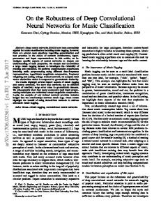
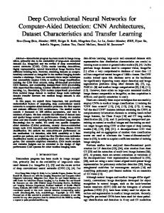
We use ConvNets with an architecture for binary image classification. Five layers of convolutional filters compute and aggregate image features. Other layers of the ConvNets perform max-pooling operations or consist of fully-connected neural networks. Our ConvNet ends with a final two-way layer with softmax probability for ‘pancreas’ and ‘non-pancreas’ classification (see Fig. 1). The fully-connected layers are constrained using “DropOut” in order to avoid over-fitting by acting as a regularizer in training Srivastava et al. (2014). GPU acceleration allows efficient training (we use cuda-convnet2 1 ).
Figure 1: The proposed ConvNet architecture. The number of convolutional filters and neural network connections for each layer are as shown. This architecture is constant for all ConvNet variations presented in this paper (apart from the number of input channels): P −ConvNet, R1 −ConvNet, and R2 −ConvNet.
2.3
P −ConvNet: Deep patch classification
We use a sliding window approach that extracts 2.5D image patches composed of axial, coronal and sagittal planes within all voxels of the initial set of superpixel regions {SRF } (see Fig. 3). The resulting ConvNet probabilities are denoted as P0 hereafter. For efficiency reasons, we extract patches every n voxels and then apply nearest neighbor interpolation. This seems sufficient due to the already high quality of P0 and the use of overlapping patches to estimate the values at skipped voxels.
2.4
R−ConvNet: Deep region classification
We employ the region candidates as inputs. Each superpixel ∈ {SRF } will be observed at several scales Ns with an increasing amount of surrounding contexts (see Fig. 4). 1
https://code.google.com/p/cuda-convnet2
4
DeepOrgan: Multi-level Deep Convolutional Networks for Automated Pancreas H. R. Roth et al. Segmentation
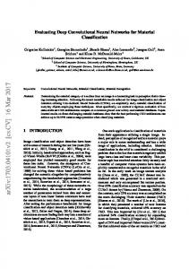
Figure 2: The first layer of learned convolutional kernels using three representations: a) 2.5D sliding-window patches (P −ConvNet), b) CT intensity superpixel regions (R1 −ConvNet), and c) CT intensity + P0 map over superpixel regions (R2 −ConvNet).
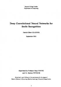
Figure 3: Axial CT slice of a manual (gold standard) segmentation of the pancreas. From left to right, there are the ground-truth segmentation contours (in red), RF based coarse segmentation {SRF }, and the deep patch labeling result using P −ConvNet. Multi-scale contexts are important to disambiguate the complex anatomy in the abdomen. We explore two approaches: R1 −ConvNet only looks at the CT intensity images extracted from multi-scale superpixel regions, and a stacked R2 −ConvNet integrates an additional channel of patch-level response maps P0 for each region as input. As a superpixel can have irregular shapes, we warp each region into a regular square (similar to RCNN Girshick et al. (2014)) as is required by most ConvNet implementations to date. The ConvNets automatically train their convolutional filter kernels from the available training data. Examples of trained first-layer convolutional filters for P −ConvNet, R1 −ConvNet, R2 −ConvNet are shown in Fig. 2. Deep ConvNets behave as effective image feature extractors that summarize multi-scale image regions for classification.
5
DeepOrgan: Multi-level Deep Convolutional Networks for Automated Pancreas H. R. Roth et al. Segmentation
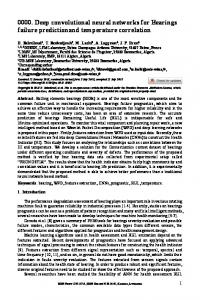
Figure 4: Region classification using R−ConvNet at different scales: a) one-channel input based on the intensity image only, and b) two-channel input with additional patch-based P −ConvNet response.
2.5
Data augmentation
Our ConvNet models (R1 −ConvNet, R2 −ConvNet) sample the bounding boxes of each superpixel ∈ {SRF } at different scales s. During training, we randomly apply non-rigid deformations t to generate more data instances. The degree of deformation is chosen so that the resulting warped images resemble plausible physical variations of the medical images. This approach is commonly referred to as data augmentation and can help avoid over-fitting Krizhevsky et al. (2012), Cire¸san et al. (2013). Each non-rigid training deformation t is computed by fitting a thin-plate-spline (TPS) to a regular grid of 2D control points {ωi ; i = 1, 2, . . . , k}. These control points are randomly transformed within the sampling window and Pk a deformed image is generated using a radial basic function φ(r), where t(x) = i=1 ci φ (kx − ωi k) is the transformed location of x and {ci } is a set of mapping coefficients.
2.6
Cross-scale and 3D probability aggregation
At testing, we evaluate each superpixel at Ns different scales. The probability P s scores for each superpixel being pancreas are averaged across scales: p(x) = N1s N i=1 pi (x). Then the resulting per-superpixel ConvNet classification values {p1 (x)} and {p2 (x)} (according to R1 −ConvNet and R2 −ConvNet, respectively), are directly assigned to every pixel or voxel residing within any superpixel ∈ {SRF }. This process forms two per-voxel probability maps P1 (x) and P2 (x). Subsequently, we perform 3D Gaussian filtering in order to average and smooth the ConvNet probability scores across CT slices and within-slice neighboring regions. 3D isotropic Gaussian filtering can be applied to any Pk (x) with k = 0, 1, 2 to form smoothed G(Pk (x)). This is a simple way to propagate the 2D slice-based probabilities to 3D by taking local 3D neighborhoods 6
DeepOrgan: Multi-level Deep Convolutional Networks for Automated Pancreas H. R. Roth et al. Segmentation
into account. In this paper, we do not work on 3D supervoxels due to computational efficiency2 and generality issues. We also explore conditional random fields (CRF) using an additional ConvNet trained between pairs of neighboring superpixels in order to detect the pancreas edge (defined by pairs of superpixels having the same or different object labels). This acts as the boundary term together with the regional term given by R2 −ConvNet in order to perform a min-cut/max-flow segmentation Boykov and Funka-Lea (2006). Here, the CRF is implemented as a 2D graph with connections between directly neighboring superpixels. The CRF weighting coefficient between the boundary and the unary regional term is calibrated by grid-search.
3
Results & Discussion
3.0.1
Data:
Manual tracings of the pancreas for 82 contrast-enhanced abdominal CT volumes were provided by an experienced radiologist. Our experiments are conducted using 4-fold cross-validation in a random hard-split of 82 patients for training and testing folds with 21, 21, 20, and 20 patients for each testing fold. We report both training and testing segmentation accuracy results. Most previous work Wang et al. (2014), Chu et al. (2013), Wolz et al. (2013) uses leave-one-patient-out cross-validation protocols which are computationally expensive (e.g., ∼ 15 hours to process one case using a powerful workstation Wang et al. (2014)) and may not scale up efficiently towards larger patient populations. More patients (i.e. 20) per testing fold make the results more representative for larger population groups. 3.0.2
Evaluation:
The ground truth superpixel labels are derived as described in Sec. 2.1. The optimally achievable DSC for superpixel classification (if classified perfectly) is 80.5%. Furthermore, the training data is artificially increased by a factor Ns × Nt using the data augmentation approach with both scale and random TPS deformations at the R−ConvNet level (Sec. 2.5). Here, we train on augmented data using Ns = 4, Nt = 8. In testing we use Ns = 4 (without deformation based data augmentation) and σ = 3 voxels (as 3D Gaussian filtering kernel width) to compute smoothed probability maps G(P (x)). By tuning our implementation of Farag et al. (2014) at a low operating point, the initial superpixel candidate labeling achieves the average 2
Supervoxel based regional ConvNets need at least one-order-of-magnitude wider input layers and thus have significantly more parameters to train.
7
DeepOrgan: Multi-level Deep Convolutional Networks for Automated Pancreas H. R. Roth et al. Segmentation
DSCs of only 26.1% in testing; but has a 97% sensitivity covering all pancreas voxels. Fig. 5 shows the plots of average DSCs using the proposed ConvNet approaches, as a function of Pk (x) and G(Pk (x)) in both training and testing for one fold of cross-validation. Simple Gaussian 3D smoothing (Sec. 2.6) markedly improved the average DSCs in all cases. Maximum average DSCs can be observed at p0 = 0.2, p1 = 0.5, and p2 = 0.6 in our training evaluation after 3D Gaussian smoothing for this fold. These calibrated operation points are then fixed and used in testing cross-validation to obtain the results in Table 1. Utilizing R2 −ConvNet (stacked on P −ConvNet) and Gaussian smoothing (G(P2 (x))), we achieve a final average DSC of 71.8% in testing, an improvement of 45.7% compared to the candidate region generation stage at 26.1%. G(P0 (x)) also performs well wiht 69.5% mean DSC and is more efficient since only dense deep patch labeling is needed. Even though the absolute difference in DSC between G(P0 (x)) and G(P2 (x)) is small, the surface-to-surface distance improves significantly from 1.46±1.5mm to 0.94±0.6mm, (p