Degenerate 3D Tensors - Semantic Scholar

Degenerate 3D Tensors Xiaoqiang Zheng1 , Xavier Tricoche2 , and Alex Pang1 1 2

University of California, Santa Cruz, CA 95064, USA University of Utah, Salt Lake City, UT 84112, USA

Abstract. Topological analysis of 3D tensor fields starts with the identification of degeneracies in the tensor field. In this paper, we present a new, intuitive and numerically stable method for finding degenerate tensors in symmetric second order 3D tensors. This method is formulated based on a description of a tensor having an isotropic spherical component and a linear or planar component. As such, we refer to this formulation as the geometric approach. In this paper, we also show that the stable degenerate features in 3D tensor fields form lines. On the other hand, degenerate features that form points, surfaces or volumes are not stable and either disappear or turn into lines when noise is introduced into the system. These topological feature lines provide a compact representation of the 3D tensor field and are essential in helping scientists and engineers understand their complex nature.

1

Introduction

Tensor fields, especially second-order tensor fields, are useful in many medical, mechanical and physical applications such as: fluid dynamics, meteorology, molecular dynamics, biology, astrophysics, mechanics, material science and earth science. Effective tensor visualization methods can enhance research in a wide variety of fields. However, developing an effective algorithm can be difficult because of the large amount of information contained in 3D tensor fields: there are nine independent components in each tensor and six for a symmetric tensor. Users in many research fields are especially interested in real symmetric tensors. In some applications, the data themselves are inherently symmetric. In other cases, symmetric tensor data can be obtained through various decomposition techniques. The main motivation and goal of this paper is to develop a simple yet powerful representation of 3D real symmetric tensor fields. Topology-based methods prove to yield simplified and effective depictions in many visualization fields. These methods consist of two general steps: identifying the critical features, and generating separatrices. Together, they divide the data space into small regions, where the hyperstreamlines form similar patterns within each one. The topological structures are simple for users to understand the underlying data fields yet sensitive enough to capture important features. In most cases, trained users can even reconstruct the data fields by looking at the topological structures. The topological structures are also a launching point for further analyses of the tensor field. For example, it forms a basis for

2

Zheng, Tricoche, Pang

seeding hyperstreamlines [7], and finding separating surfaces that partitions the data in regions with similar properties. Early work on using topology-based method to visualize tensor fields by [1,2] lays an important background for this research project. It defines the tensor topology based on degenerate features and discusses its nature for the 2D case in great detail, and provides useful knowledge for the 3D case. But we find this early work insufficient in studying 3D tensor topology. Not only is the dimensionality of the features unknown, but how to numerically extract the topological structures is also obscure. In their previous work, Hesselink et al. mentioned that the dimension of the degenerate features can be points, lines, surfaces or subvolumes. This claim itself is essentially true, but it does not point out the dimension of features in a typical nondegenerate 3D tensor. By analogy, although the critical features in 3D vector fields can be lines, surfaces or even subvolumes, we know they are mostly isolated points in a typical non-degenerate vector field. This knowledge is the foundation for the study of topological structure in vector visualization. All the subsequent study on separatrices and other topological features are based on the extraction of the critical points. On the other hand, no topological results on 3D real symmetric tensor fields been published to date indicating that topological tensor features form lines. Our recent research [9] indicates that the degenerate features in 3D tensor fields form feature lines that are stable even in the presence of noise. In the next section, we discuss the dimensionality of features in 3D tensor fields. Then, we quickly review the traditional method of finding degenerate features in 3D tensors fields based on discriminants, followed by the constraint function approach presented in [9]. Both of these methods are considered implicit functional approaches. This is followed by a presentation of our new method based on the geometric interpretation of a tensor.

2

Dimensionality of Degenerate Features

Similar to the 2D case described in the previous chapter [8], a 3D real symmetric tensor can be decomposed into three orthogonal eigenvectors, each of which has a real eigenvalue associated with it. They are labeled as major, medium and minor eigenvectors according to the relative order of their eigenvalues. A degenerate tensor is obtained when two or more of the eigenvalues are equal. The corresponding position in the tensor field is called a degenerate point. It follows that degenerate points are the only places where hyperstreamlines can cross each other. As mentioned in introduction, the purpose of a topological analysis is to divide the data space into regions where hyperstreamlines show a similar pattern. Therefore the collection of these degenerate points constitutes the topological features of interest. Although the experience in flow visualization shows that a visualization restricted to topology alone may be incomplete and ignore essential features like vortex core

Degenerate 3D Tensors

3

lines, this analysis remains an important step toward better understanding of the complicated nature of 3D tensor data.

Before we can extract these topological features from 3D tensor fields, we need to know their dimension. Algorithms to locate points, lines, surfaces and volumes employ very different strategies. During our earlier work [9] we discovered that for most non-degenerate 3D tensors, the dimensionality of the critical feature is one, i.e. the collection of degenerate points form feature lines. This conclusion can be shown using an early theorem by von Neumann and Wigner which states that the real symmetric degenerate matrices form a variety of codimension two [5]. Codimension is defined as the difference between the dimension of a space and the dimension of a subspace contained in it. 3D real symmetric tensors have six independent components. Therefore they form a tensor space of dimension six. A double degenerate tensor where two eigenvalues are equal can be uniquely specified using four parameters. In other words, double degenerate tensors form a subspace A of dimension four in 6D tensor space. In a typical non-degenerate setting, tensor fields defined in a 3D space usually form a subspace B of dimension three in the same 6D tensor space. The degenerate tensors are then the intersection of these two subspaces. It can be shown by transversality that these dimensions satisfy the following formula: codim(A ∩ B) = codim(A) + codim(B), which yields codim(A∩B) = 2+3 = 5, that is this intersection usually has a dimension one, i.e. forms lines. From the same line of reasoning, we known that degenerate tensors are isolated points in most cases if the data is specified in a 2D space. Since most numerical algorithms are designed to capture points, the basic block of our feature extraction algorithm is to locate 3D degenerate tensors on a 2D patch and then to connect them into lines afterwards.

While the main features are lines, it is still possible to obtain features that are points, surfaces or subvolumes. Features that form points, surfaces or subvolumes are less common in most 3D tensor fields and are usually induced by symmetry constraints. Such features are considered unstable and do not persist under perturbation. For example, a triple degenerate point where three eigenvalues are equal can be uniquely specified using one parameter (scaling of an identity matrix). In this case, previous computation yields a codimension 5 + 3 = 8 > 6, which results in an unstable feature. Hence we focus our tensor feature extraction on feature lines rather than surfaces or subvolumes. We still need to extract points as these form the basis for the feature lines. Because of this design criterion, features that are surfaces (e.g. in the single point load data) or subvolumes may not be detected as readily as feature lines. This limitation is not insurmountable, but is rather based on the effective use of limited resources in finding features that are not as common nor as stable.

4

3

Zheng, Tricoche, Pang

Implicit Function Approach

The first family of methods to analyze degenerate tensors is through implicit functions. In this family, a tensors is degenerate if and only if its value makes an implicit function equal zero. Here we introduce two formulations: discriminant and constraint function. Note that since degenerate tensors form a variety of codimension two, an ideal formulation of the implicit constraint defining degenerate tensors should have two implicit functions. But neither of the two formula shown below has this property. 3.1

Discriminants

Hesselink et al. show that the only degenerate features are those having at least two equal eigenvalues [2]. Fortunately, we do not need to conduct the eigen decomposition to find the degenerate points. A tensor has two (or three) equal eigenvalues if and only if its discriminant equals zero. The discriminant D3 of a tensor T with eigenvalues λ1 , λ2 and λ3 is defined as,   T00 T01 T02 T =  T01 T11 T12  (1) T02 T12 T22 D3 (T ) = (λ1 − λ2 )2 (λ2 − λ3 )2 (λ3 − λ1 )2

(2)

This can be reformulated into a form that does not require eigen decomposition to determine eigenvalues as follows: P =

T + T11 + T22 ¯ ¯ 00¯ ¯ ¯ ¯ ¯ T00 T01 ¯ ¯ T11 T12 ¯ ¯ T22 T02 ¯ ¯ ¯ ¯ ¯ ¯ ¯ Q=¯ + + T01 T11 ¯ ¯ T12 T22 ¯ ¯ T02 T00 ¯ ¯ ¯ ¯ T00 T01 T02 ¯ ¯ ¯ ¯ T01 T11 T12 ¯ R= ¯ ¯ ¯ T02 T12 T22 ¯

D3 (T ) = Q2 P 2 − 4RP 3 − 4Q3 + 18P QR − 27R2

(3) (4) (5)

(6)

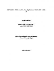
From Equation 2, we can easily find that a discriminant is (a) always non-negative; (b) equal to zero if and only if at least two of the eigenvalues are equal. And it is ideal for computation and numerical purposes because although it is defined on eigenvalues, we do not really need to carry out an expensive eigen decomposition. Instead, we only need to compute Equation 6 which is a polynomial of order six to get the discriminant. An interesting geometric mapping of the three real eigenvalues is the Cardano circle or the eigenwheel. This is illustrated in Figure 1 where the three

Degenerate 3D Tensors

5

roots are the x-intercepts of the three axes that are 120 degrees apart. Note that the roots λ1 , λ2 and λ3 are increasing from left to right. The angle of the axes associated with the largest eigenvalue and the positive X axis is labeled as α. It is obvious that a double degeneracy occurs when α = 0 resulting in λ1 = λ2 , and α = 180 resulting in λ2 = λ3 . We refer to the first type of double degeneracy as Type B, and the second type of double degeneracy as Type A. A triple degenerate point occurs when all three eigenvalues are equal and zero, and the radius of the circle also reduces to zero. A very rare event indeed.

λ2 λ3 α

λ1

(a)

λ1λ2

(b)

λ3

λ1

λ2λ 3

(c)

Fig. 1. Cardano’s circle. (a) Relative positions of eigenvalues along the x-axis, (b) type B double degenerate point where the minor and medium eigenvalues are equal, and (c) type A double degenerate point where the medium and the major eigenvalues are equal.

3.2

Constraint Functions

In [9], an alternative formulation of degenerate points leading to a more stable numerical solution was presented. We briefly highlight the results here. Although Equation 6 provides an elegant representation for evaluating the discriminant without having to perform eigen decomposition, it is difficult to solve. In Equation 6, the discriminant of a real symmetric tensor is a polynomial of order six. Since it is always non-negative, the degenerate tensor also happens to be its minimum. Rather than using a minimization approach to find the degenerate tensors, the numerical analysis community recommends a root-finding strategy such as conjugate gradient for better numerical stability. A good method widely used to find the root of an equation is to detect the change of signs and then to recursively bisect the domain of interest. But because the degenerate feature is itself a minimum, there is no change of sign at all. Relying on the gradients is also dangerous, because the gradients are notoriously unstable unless they are very close to the feature. Due to this high-orderedness and singularity, directly finding the root

6

Zheng, Tricoche, Pang

of a cubic discriminant stably is very difficult. Instead, we look for another representation of the discriminant. In our previous investigation, we found that while Hilbert [3] pointed out that not all non-negative polynomials can be broken down into the sum of squares of polynomials, the cubic discriminant can be written as the sum of the squares of seven polynomials. We also learned that not only can the discriminant of a second-order tensor of any dimension be expressed as the sum of squares [4], but our solution to the 3D case of seven equations is optimal [6]. Therefore, the definition of degenerate tensors can also be expressed as the tensors where the seven constraint functions are all zero at the same time. We use these seven cubic equations to extract the feature lines from 3D tensor fields. The seven discriminant constraints are: 2 2 2 2 2 2 fx (T ) = T00 (T11 − T22 ) + T00 (T01 − T02 ) + T11 (T22 − T00 )+ 2 2 2 2 2 2 ) − T12 ) + T22 (T02 − T11 ) + T22 (T00 − T01 T11 (T12 2 2 2 2 fy1 (T ) = T12 (2(T12 − T00 ) − (T02 + T01 ) + 2(T11 T00 + T22 T00

−T11 T22 )) + T01 T02 (2T00 − T22 − T11 ) 2 2 2 2 fy2 (T ) = T02 (2(T02 − T11 ) − (T01 + T12 ) + 2(T22 T11 + T00 T11 −T22 T00 )) + T12 T01 (2T11 − T00 − T22 ) 2 2 2 2 fy3 (T ) = T01 (2(T01 − T22 ) − (T12 + T02 ) + 2(T00 T22 + T11 T22 −T00 T11 )) + T02 T12 (2T22 − T11 − T00 )

fz1 (T ) = fz2 (T ) =

2 2 ) + T01 T02 (T11 − T22 ) − T01 T12 (T02 2 2 ) + T12 T01 (T22 − T00 ) − T12 T02 (T01

fz3 (T ) =

2 2 T01 (T12 − T02 ) + T02 T12 (T00 − T11 )

D3 (T ) = fx (T )2 + fy1 (T )2 + fy2 (T )2 + fy3 (T )2 + 15fz1 (T )2 + 15fz2 (T )2 + 15fz3 (T )2

(7)

A tensor is degenerate if and only if all of its seven constraint functions are zero. This is the condition that we employ to extract the critical features in 3D tensor fields. Its first advantage is that the constraint functions are only cubic polynomials, instead of a polynomial of order of six which tend to oscillate more. This property leads to a more stable and accurate numerical algorithm. In addition, the requirement that all seven constraint functions be zero at the same time depends on the tensor value only and not on the gradient calculated from adjacent tensors. Hence, the algorithm yields a more accurate result than the algorithms that rely on finding critical points where the gradients of the discriminants are zeros. Its second advantage is that the constraint functions can be both positive or negative, as opposed to always being non-negative. This property allows us to perform a fast and inexpensive check for the existence of features. And finally, the reformulation also does not require eigen decomposition.

Degenerate 3D Tensors

(a) Two degenerate points

7

(b) Three degenerate points

Fig. 2. White dots are degenerate points indicating places where all seven constraint functions are zero. Each colored curve corresponds to a constraint function being equal to zero. Places where multiple curves intersect are where multiple constraint functions are satisfied simultaneously. The background is pseudo-colored by the discriminant functions. The data is a 2D slice of a randomly generated 3D tensor field.

To find these degenerate points, we employ an iterative root finding method that satisfies all seven constraints simultaneously. Assume the tensor −−→ field at location X is T (X). For the feature points X ∗ , we have CF (X ∗ ) = − − → CFi (X ∗ ) = 0, for i = 1, ..., 7, where CF (X) is an assembly of the seven constraint functions into one vector function. Using the Newton-Raphson method and an initial guess of Xn , we have the following conceptual algorithm,

Xn+1

¯ µ −−→ ¶−1 ¯ −−→¯ ∂ CF · CF = Xn − ¯ ∂X ¯ ¶−1 X=X¯¯n µ −−→ −−→¯ ∂T · CF ¯ = Xn − ∂ CF ∂T · ∂X ¯

(8)

X=Xn

−−→ −−→ CF from the chain rule using ∂ CF and ∂T Note that we calculate the ∂∂X ∂T ∂X −−→ rather than from the interpolated values of CF on the grid using finite differ−−→ ence methods for higher precision. ∂ CF is calculated from the formula of the ∂T

∂T tensor constraints, and ∂X is from the interpolated tensor values. We used both the bilinear and bicubic natural spline interpolations. However, Equation 8 does not work because on a cell face, X is only 2D −−→ −−→ while CF is 7D. Thus, ∂ CF is a 7 × 2 matrix. There are a number of ways to ∂X

8

Zheng, Tricoche, Pang

deal with such a system. In our case, we find that the least square estimator involving the transpose of the matrix works quite well. à −−→ T !¯¯ −−→ !−1 à −−→ T ∂ CF ∂ CF ∂ CF −−→ ¯ (9) Xn+1 = Xn − · · CF ¯¯ ∂X ∂X ∂X ¯ X=Xn

This new hybrid algorithm minimizes the square error terms among the seven constraints. Using the center of each cell as the initial guess for an intersection point, we find that this method converges to the actual intersection point within five iterations in most non-degenerate cases with precisions up to 10−9 , and it almost never misses a feature point if it exists. Additional points are obtained by subdividing the cell face. This Newton-Raphson based method on constraint functions is superior in speed, accuracy and precision compared to other methods developed directly based on the cubic discriminants. For example, we also implemented a comparison algorithm based on cubic discriminant that searched for its minimum using conjugate gradient methods. Not only is it about 50 times slower, using any precision less than 10−6 will yield a false negative rate of over 50%.

4

Geometric Approach

Since we want to extract the degenerate tensors in a root-finding framework, it is desirable to have a system of equations with an equal number of equations as there are unknowns. However, neither the discriminant nor the constraint functions satisfy this condition. An equation based on discriminant is underspecified since there is only one equation but with two unknowns. An equation based on constraint functions is over-specified because there are seven equations with two unknowns. The formulation on constraint functions is better than its discriminant counterpart numerically because an over-specified system is easier to solve using the modified Newton-Raphson algorithm and achieves high convergence rates and precision. In this section, we present another extraction algorithm based on the geometric properties of 3D tensors that meets the desired criterion of a well defined system. Theorem 1. A tensor T is degenerate if and only if it can be written as the sum of a spherical tensor and a linear tensor (see Figure 3). The sufficiency of this theorem is easy to prove. To show its necessity, we simply subtract the duplicate eigenvalues from the diagonal components of the tensor. It is easy to show that the remaining tensor has two duplicate zero eigenvalues. In other words, the rank of the remaining tensor is at most rank one, i.e., linear. Depending on the sign of the other eigenvalue, a linear real symmetric tensor can always be written as the product of a vector, its transpose and an extra sign. This gives us a simple way to write a degenerate tensor,

Degenerate 3D Tensors

9

Fig. 3. Relationship between s and V and the degenerate tensor glyph.

T = sI ± V · V T

(10)

where s is a scalar, I is a 3 × 3 identity matrix and V is a 3 × 1 vector. An advantage of this formula is that it can distinguish between type A and type B double degenerate points: T is type A with equal major and medium eigenvalues if the minus sign holds; and T is type B with equal minor and medium eigenvalues if the plus sign holds. In applications where the users are only interested in the major hyperstreamline topology, users only need to keep the minus sign, since the major hyperstreamlines are only degenerate at type A features. The three eigenvalues are: λ1 = λ2 = s, and λ3 = s ± kV k2 . One of the eigenvectors is e3 = V /kV k and the other two eigenvectors are any two orthogonal vectors that are also perpendicular to e3 . Besides its simplicity, this equation also clearly states that all 3D degenerate tensors form a fourparameter family. A typical and non-degenerate 3D real symmetric tensor on a 2D patch parameterized by (x, y) is, T (x, y) = sI ± V · V T

(11)

Since there are six independent components in real symmetric tensors, this system of equations has six equations and six unknowns. Therefore we expect that it has stable and isolated solutions. If we assume that the tensor patch is obtained through bilinear interpolation, each equation is quadratic. It is another intuitive and geometric explanation that 3D degenerate tensors are stable on 2D tensor patch and form lines in 3D tensor field. To solve it, we can employ any standard numerical methods to solve an equally-specified system of equations such as Newton-Raphson algorithm and its variants. For the initial guess in the Newton-Raphson method, we use the center of the patch, (x0 , y0 ), in place of the position parameters (x, y). Suppose the tensor at (x0 , y0 ) is T0 and suppose that its eigenvalues are (λ1 ≤ λ2 ≤ λ3 ) and its normalized eigenvectors are (e1 , e2 , e3 ), respectively. Without loss of generality, we also assume that we are extracting type A degenerate features. The algorithm for extracting type B degenerate features is similar in form. To obtain the initial estimates of the other four parameters (s, V ), we use the following heuristic,

10

Zheng, Tricoche, Pang

λ2 + λ 3 p 2 V0 = s 0 − λ 1 · e1 s0 =

(12) (13)

Using s0 and V0 for the initial guess, we iteratively update the six parameters using the Newton-Raphson method until the solution converges. Since each equation is a simple quadratic equation, taking derivatives is trivial. When the algorithm converges, not only do we have the location of the degenerate feature, but we also get the eigenvalues and eigenvectors of the tensor values at that point from s and V . Besides its simplicity, the disadvantage of this algorithm is also obvious – we need to invert a 6 × 6 matrix during each iteration of the Newton-Raphson algorithm. A less obvious disadvantage is that in our experiments, this algorithm shows worse numerical stability than the algorithms built on the constraint functions in situations when the features are very close to triple degeneracy. A useful form of 3D tensor is the deviator. It is simply a 3D tensor whose trace is zero, which implies that the sum of the eigenvalues is also zero. We can obtain the deviator part of any 3D tensor T by subtracting one third of its trace from its three diagonal components. Since this is a linear operation, the zero-trace property is preserved on a discrete grid using trilinear interpolation. One variation of the basic geometric algorithm is to consider only the deviator field of the original tensors. For the case of extracting type A degenerate features, it is easy to get, Vx2 + Vy2 + Vz2 (14) 3 Substituting this term back into Equation 11 and throwing away any redundant diagonal equation, we get a system with five equations and five unknowns. In our experiments, we found that this variation is almost equivalent to the original algorithm in terms of numerical stability and convergence speed. s=

5

Topological Feature Lines

Now that we have obtained the degenerate points using one of the methods described in the two previous sections, the next step is to form the topological feature lines. The general idea is to connect the degenerate points on cell faces with those at neighboring cell faces. However, as we can clearly see in Figure 2, some cells may have more than one degenerate point, and hence more than one feature line going though them. We therefore use a multi-pass approach to connect these degenerate points. The procedure proceeds by examining only those candidate cells that contain degenerate points (i.e. intersection

Degenerate 3D Tensors

11

points of feature lines with the face) on at least one of their six faces. In the first pass, all candidate cells containing exactly two intersection points are processed by: (a) simply connecting those two points, (b) recording the orientation of the line segment as tangents at the end points, and (c) marking the cell as processed. In the subsequent passes, their unprocessed neighboring candidate cells are processed by connecting a line segment between each pair of intersection points in such a way as to minimize the angle deviation between the tangent recorded at the end point and the line towards other intersection points within the cell. Each neighboring candidate cell is marked as processed, and the procedure continues until there are no more candidate cells. In our current implementation, we use this iterative method to generate the tangent lines on topological feature points and ultimately resolve the line connections between multiple points. In the future, we plan to calculate the tangent of the degenerate tensor line at a specific feature point analytically instead of this post-processing method.

6

Results

We experimented with four data sets to test out our degenerate tensor extraction algorithm using the geometric approach. In the experiments, we use a pre-filtering algorithm that is similar to the one used in [9]. The first is a 2D rectangular patch with symmetric 3D tensors at the four corners that have been set randomly (see Figure 2). The tensor values within the patch are obtained through linear interpolation. This synthetic data corresponds to tensors on a face of a 3D cell. The second is a 3D cell with symmetric 3D tensors on its eight corners which are also set randomly (see Figure 4). It is sampled into a higher resolution for smoother features lines. The third is the stress tensor data in a semi-infinite volume with two point loads (see Figure 5). The fourth is the deformation tensors in the computed flow past a cylinder with hemispherical cap (see Figure 6). From Figures 4 to 5, the colors of the volumes are mapped to the tensor discriminant (Equation 6) with blue mapped with lower transparency to zero and warmer colors with higher transparency mapped to higher values. Degenerate tensors can be found in the blue regions. Additional digital images can be accessed online at: www.cse.ucsc.edu/research/avis/tensortopo.html. Figure 4 shows degenerate tensors in a 3D cell form feature lines (rendered as tubes). Note that the feature lines are not hyperstreamlines, rather they are where the major and medium, or the medium and minor, or all three hyperstreamlines intersect each other. Only the faint green is visible in the vicinity of the tubes because the tubes are in the blue regions. The color of the tubes are such that type A points with very different minor value are mapped to warmer colors, and type B points with very different major value are mapped to cooler colors. The milder colors are where the other eigenvalue

12

Zheng, Tricoche, Pang

is not as different as the degenerate pair. We see that complex feature lines can form even from a simple linearly interpolated random tensor field.

(a) First set

(b) Second set

Fig. 4. Randomly generated 3D tensors. Warmer line colors are closer to type A degenerate points where major and medium hyperstreamlines intersect, while cooler line colors are closer to type B degenerate points where medium and minor hyperstreamlines intersect. The rest of the volume is pseudo-colored by the discriminant using cool colors for low discriminant values (closer to feature lines) and warm transparent colors for distant values.

Figure 5 shows the double point load stress tensors. The yellow arrows indicate the two point loads, and the two magenta spheres are the triple degenerate points. We can see the line of double degeneracy connecting these two stress-free points as alluded to in [2]. Other very interesting feature lines are also extracted. The first is a vertical loop that lies directly under the double degenerate feature line connecting the two triple degenerate points. This feature is not present in the single point load data. This loop feature is also stable in the sense that it persists even as the relative magnitudes of the two point loads are varied. The second is how the blue feature line below each of the point load bifurcate and then reconnect. These two structures and the vertical loop are connected together by a type A feature line running between the two point loads. Looking from the top view in (b), we see another interesting feature which is the circular feature line that connects the two point loads and the two triple degenerate points. It is worth noting that the stress tensor is dominated by only one single load in the vicinity of the load point, so it is locally similar to the single point load stress tensor where the degenerate tensor form a surface symmetrically spreading away from the

Degenerate 3D Tensors

13

load point. Since our algorithm is designed for extracting features lines, it produces artifacts when the features form a surface or subvolume.

(a) Oblique view

(b) Top view

Fig. 5. Double point load data. Yellow arrows indicate point load, while the 2 magenta spheres show the location of the triple degenerate points. Color scheme is the same as Figure 4.

Figure 6 shows degenerate lines in the deformation tensors of the computed flow past a cylinder with a hemispherical cap. Only a portion of the data close to the cap is shown because most of the interesting features are found there. First, we see a curved line on the cap shown by the black arrow. It matches some of the patterns of the velocity topology from the same data set. There are more features at the upper half of the data because the flow there is more turbulent. Figure 6(a) is from an oblique view. Most of the features are close to the geometry of the object except a complicated branch structure which extends away from the geometry. It contains a small cyan horn shape pointed by the pink arrow, two green ring shapes, and a bifurcating structure. Figure 6(b) is from a top view. We also see a strong type B (blue) bulb shape structure that extends to the end of the cylinder. Near the cap, it intertwines with a strong type A (red) heart shape structure. This phenomenon is interesting in that although these two structures are very close, they do not cross each other. It also means the tensors are quite turbulent in this area, because large variations are happening in very close proximity. The time statistics for the different data sets are summarized in Table 6.

14

Zheng, Tricoche, Pang

(a) Oblique View

(b) Top View

Fig. 6. Degenerate lines in deformation tensors of flow past a cylinder with a hemispherical cap. Feature lines are colored as in Figure 4. Data Set Time 2D Random Patch (1 × 1) 0.05 (millisec) 3D Random Cell (32 × 32 × 32) 0.9 (sec) Double Point Load (64 × 64 × 64) 4.2 (sec) Hemisphere (72 × 110 × 84) 23 (sec) Table 1. Time to extract degenerate tensors in different datasets

7

Open Problems

There are many open problems that need to be investigated. We highlight a few of them here. First, since all the algorithms are built on extracting lines, they have problems dealing with features that form surfaces and volumes. Finding the separatrices of these features would also need to be addressed. Second, in our numerical algorithms, we define the degenerate tensors as points with two equal eigenvalues without considering the eigenvectors. But we are originally interested in these points because they are where hyperstreamlines can cross each other, and hyperstreamlines are defined on eigenvectors. Therefore, a proper definition or an extraction algorithm based on both eigenvalues and eigenvectors could provide more insight into this problem. At each point along the degenerate lines, we can project the 3D tensors onto a 2D plane perpendicular to the eigenvector with distinct eigenvalue [7].

Degenerate 3D Tensors

15

The projected 2D tensors also show a degenerate pattern. One can extract the separatrix of the 3D tensor field by calculating the separatrices of the projected 2D tensors at each point and connecting them together. With the 3D degenerate tensors and their separatrix surfaces, we will have a complete topological structure of 3D tensor fields. Simplification and tracking of the topological structure proved to be useful for 2D tensor fields [8]. In 3D, they are more difficult since the degenerate features become lines instead of points. Finally these techniques should be extended to other application domains such as diffusion tensor MRI data described in other chapters of this book. While the main attribute of interest is usually the path of the fibers, highly linear fibers are where we would likely find feature lines. Hence, it is possible that topological visualization of DT-MRI data would also be beneficial. For this approach to be of real practical interest, the issue of topological artifacts induced by noisy data must be addressed as well.

8

Acknowledgment

This work is supported by NSF ACI-9908881. The flow data is courtesy of NASA. We would also like to thank Peter Lax and Beresford Parlett for their correspondence.

References 1. T. Delmarcelle and L. Hesselink. The topology of second-order tensor fields. In R.D. Bergeron and A.E. Kaufman, editors, Proceedings IEEE Visualization ’94, pages 140–148. IEEE Computer Society Press, 1994. Flow Features and Topology. 2. L. Hesselink, Y. Levy, and Y. Lavin. The topology of symmetric, second-order 3D tensor fields. IEEE Transactions on Visualization and Computer Graphics, 3(1):1–11, Jan-Mar 1997. ˘ 3. D. Hilbert. Uber die darstellung definiter formen als summen von quadraten. Math. Annalen, 32:342–350, 1888. 4. P. D. Lax. On the discriminant of real symmetric matrices. Communications on Pure and Applied Mathematics, LI:1387–1396, 1998. 5. Peter Lax. Linear Algebra. Wiley, 1996. 6. B. N. Parlett. The (matrix) discriminant as a determinant. Linear Algebra and its Applications, 355:85–101, 2002. 7. Wei Shen. Seeding strategries for hyperstreamlines. Master’s thesis, University of California, Santa Cruz, 2004. 8. Xavier Tricoche, Xiaoqiang Zheng, and Alex Pang. Visualizing the Topology of Symmetric, Second-Order, Time-Varying Two-Dimensional Tensor Fields, page XXX. Springer, 2005. 9. Xiaoqiang Zheng and Alex Pang. Topological lines in 3D tensor fields. In Proceedings of Visualization 04, Austin, 2004. to appear.