Delay-induced synchronization phenomena in an array of globally ...

PHYSICAL REVIEW E 67, 056219 共2003兲

Delay-induced synchronization phenomena in an array of globally coupled logistic maps A. C. Martı´ and C. Masoller

Instituto de Fı´sica, Facultad de Ciencias, Universidad de la Repub´lica, Igua´ 4225, 11400 Montevideo, Uruguay 共Received 6 December 2002; published 27 May 2003兲 We study the synchronization of a linear array of globally coupled identical logistic maps. We consider a time-delayed coupling that takes into account the finite velocity of propagation of the interactions. We find globally synchronized states in which the elements of the array evolve along a periodic orbit of the uncoupled map, while the spatial correlation along the array is such that an individual map sees all other maps in his present, current, state. For values of the nonlinear parameter such that the uncoupled maps are chaotic, time-delayed mutual coupling suppresses the chaotic behavior by stabilizing a periodic orbit that is unstable for the uncoupled maps. The stability analysis of the synchronized state allows us to calculate the range of the coupling strength in which global synchronization can be obtained. DOI: 10.1103/PhysRevE.67.056219

PACS number共s兲: 05.45.Xt, 05.65.⫹b, 05.45.Ra

I. INTRODUCTION

Coupled oscillator models are widely used to model complex dynamics in nonequilibrium extended systems, and their synchronization has attracted a lot of attention in recent years 关1兴. In studies of coupled ensembles of nonlinear oscillators, different situations have been considered 共identical or nonidentical units, periodic or chaotic single-unit behavior, local or global coupling兲, and a rich variety of synchronization phenomena has been found 共for a recent review, see Ref. 关2兴兲. In the field of coupled map lattices, the paradigmatic model, originally introduced by Kaneko 关3,4兴, is the ensemble of N logistic maps with mean field global coupling:

⑀ x i 共 t⫹1 兲 ⫽ 共 1⫺ ⑀ 兲 f 关 x i 共 t 兲兴 ⫹ N

N

兺

j⫽1

f 关 x j 共 t 兲兴 ,

共1兲

i苸 关 1,N 兴 , f (x)⫽ax(1⫺x), and ⑀ is the coupling strength. For relatively large coupling, global 共full兲 synchronization occurs: the array synchronizes on the manifold x 1 ⫽••• ⫽x N , where the dynamics of an element is generated by the uncoupled map. For weaker coupling, cluster 共or partial兲 synchronization occurs: the array splits into K clusters of N 1 , . . . ,N K elements mutually synchronized 关5,6兴. A characteristic of many biological and physical systems is time-delayed coupling in the interaction among many units. Two different situations can be distinguished: when the retardation time in the coupling is the same for all the units, and when the retardation time is different for the different units. An example of the first case was studied in Refs. 关7,8兴, which considered an array of diode lasers with delayed coupling via an external reflector. The retardation time in the coupling is the same for all lasers since it given by the external cavity round-trip time. The delay time was found to induce in-phase synchronization of the array; a behavior that was interpreted in terms of generalized Kuramoto phase equations. Globally coupled logistic maps with time-delay interactions were studied in Ref. 关9兴; the maps were coupled with the same delay k: 1063-651X/2003/67共5兲/056219共6兲/$20.00

⑀ x i 共 t⫹1 兲 ⫽ 共 1⫺ ⑀ 兲 f 关 x i 共 t 兲兴 ⫹ N

N

兺

j⫽1

f 关 x j 共 t⫺k 兲兴 .

共2兲

The dynamics of the array was found to be strongly sensitive to the value of the delay time, which can increase the probability of the cluster state for small coupling strengths, and can also break up the cluster state for large coupling. Suppression of spatiotemporal chaos in a linear array with local 共nearest neighbor兲 coupling, via local and global timedelayed feedback was demonstrated numerically and analytically in Refs. 关10,11兴. In the case of globally coupled units, the introduction of distance-dependent time delays makes the spatial coordinates of an element relevant in spite of the infinite range of the mean-field interaction. This situation was considered in Ref. 关12兴 for one-dimensional arrays of coupled phase oscillators. It was shown that in the limit of short delays, the ensemble approaches a state of frequency synchronization, and that this state might develop a spatial nontrivial distribution of phases. In two-dimensional arrays, distance-dependent time delays induce a variety of patters including traveling rolls, steady patterns, spirals, and targets 关13兴. Here we study the effects of distance-dependent retarded coupling in a linear array of logistic maps:

⑀ x i 共 t⫹1 兲 ⫽ 共 1⫺ ⑀ 兲 f 关 x i 共 t 兲兴 ⫹ N

N

兺

j⫽1

f 关 x j 共 t⫺ ␶ i j 兲兴 ,

共3兲

where ␶ i j ⫽k 兩 i⫺ j 兩 is proportional to the distance between the ith and jth maps and k is the inverse of the velocity of the signal that travels through the array. In a previous work 关14兴, we considered the case in which the uncoupled maps evolve in a periodic orbit of period 2 共when 3⭐a⭐1 ⫹ 冑6). We found that for weak coupling the array divides into clusters, and the behavior of the individual elements within each cluster depend on the delay times. For strong enough coupling global synchronization occurs, where the dynamics of an element is periodic of period 2, generated by the uncoupled logistic map. The spatial correlation of the elements along the array is such that if k is even, at time t all elements are in the same state, while if k is odd, at time t

67 056219-1

©2003 The American Physical Society

A. C. MARTI´ AND C. MASOLLER

PHYSICAL REVIEW E 67, 056219 共2003兲

neighboring elements are in different states. In both cases an individual map sees all other maps in its present, current, state. In this paper we extend the previous study and consider that the uncoupled maps can be either periodic or chaotic 共i.e., 3⭐a⭐4). We find that for adequate coupling strength and time delay, global synchronization occurs. In the globally synchronized state all elements evolve along a periodic orbit of the uncoupled logistic map. Remarkably, this orbit might be unstable for the uncoupled maps. In particular, when the uncoupled maps are chaotic, time-delayed coupling might suppress chaos, stabilizing an unstable periodic orbit. For small arrays we study the stability of the globally synchronized solution and calculate the minimum coupling strength above which the unstable orbit of the uncoupled maps becomes stable for the time-delayed coupled maps. The numerical simulations are in excellent agreement with the stability analysis. This paper is organized as follows. In Sec. II we analyze the existence and the stability of the globally synchronized state. In Sec. III we present results of the numerical simulations and the stability analysis. Finally, in Sec. IV we present a summary and the conclusions.

the antiphase solution has to be even. The in-phase and antiphase solutions verify Eq. 共6兲 only for certain delay times. For the in-phase solution, mod共 ␾ i ⫺ ␾ j , P 兲 ⫽mod共 k 兩 i⫺ j 兩 , P 兲 ⫽0

᭙ i and j only if k⫽n P, with n an integer number; for the antiphase solution, mod共 ␾ i⫹1 ⫺ ␾ i , P 兲 ⫽mod共 k, P 兲 ⫽ P/2

y im 共 t 兲 ⫽x i 共 t⫺m 兲 ,

y im 共 t⫹1 兲 ⫽

N

⑀ 共 1⫺ ⑀ 兲 f 关 y i0 共 t 兲兴 ⫹ 兺 f 关 y j,k 兩 j⫺i 兩 兴 , N j⫽1

if m⫽0. 共11兲

共5兲

Next we define the vector Z⫽ 共 y 10 ,y 20 , . . . ,y N0 ;y 11 ,y 21 , . . . ,y N1 ; . . . ; ⫻y 1M ,y 2M , . . . ,y NM ),

共6兲

Z A1 ⫽ 共 x a ,x b , . . . ;x b ,x a , . . . 兲 , Z A2 ⫽ 共 x b ,x a , . . . ;x a ,x b , . . . 兲 ,

共13兲

and the in-phase solutions of period 2 as Z I1 ⫽ 共 x a ,x a , . . . ;x b ,x b , . . . 兲 ,

for all i and j, where m i j are arbitrary integer numbers. The symmetry of the delays, ␶ i j ⫽ ␶ ji , implies that

Z I2 ⫽ 共 x b ,x b , . . . ;x a ,x a , . . . 兲 ,

共7兲

Thus, the phase differences ␾ i ⫺ ␾ j cannot be arbitrary, but have to be either ␾ i ⫺ ␾ j ⫽n i j P or ␾ i ⫺ ␾ j ⫽ P/2⫹n i j P, with n i j an integer number. We shall refer to solutions with mod( ␾ i ⫺ ␾ j , P)⫽0 ᭙ i and j as in-phase solutions, and solutions with mod( ␾ i⫹1 ⫺ ␾ i , P)⫽ P/2 ᭙ i as antiphase solutions. Since mod( ␾ i⫹1 ⫺ ␾ i , P) is an integer number, the period P of the orbit for

共12兲

which has N(M ⫹1) components. The antiphase solutions of period 2 can be written as

with x 0 (t) a particular realization of the limit cycle, used as a reference orbit. The condition for this solution to satisfy the evolution equation is

␾ i ⫺ ␾ j ⫹m i j P⫽ ␾ j ⫺ ␾ i ⫹m ji P.

再

y i,m⫺1 共 t 兲 , if m⫽0,

共4兲

Thus, each element ‘‘perceives’’ the array as being fully synchronized, in spite of the fact that the simultaneous states of different elements might not coincide. In these globally synchronized solutions, each element evolves along a limit cycle of period P of the uncoupled logistic map with a given phase, such that we can write

␾ i ⫺ ␾ j ⫹m i j P⫽ ␶ i j ⫽k 兩 i⫺ j 兩

共10兲

where 1⭐i⭐N and 0⭐m⭐M with M ⫽max(␶ij). In terms of these new variables, Eq. 共3兲 becomes

A special class of solutions of Eq. 共3兲 is characterized by the fact that, for all pairs i, j, the signal received by map i at each time corresponds to a delayed state of map j, which coincides with the present state of map i:

x i 共 t 兲 ⫽x 0 共 t⫹ ␾ i 兲 ,

共9兲

only if k⫽ P/2⫹n P, with n an integer number. The existence of these globally synchronized states is independent of the coupling strength; the only requirement is that the periodic orbit is a solution 共stable or unstable兲 of the logistic map. To analyze the stability of the globally synchronized solutions, we turn the delayed equation 共3兲 into a nondelayed equation by the introduction of auxiliary variables:

II. GLOBALLY SYNCHRONIZED SOLUTIONS

x j 共 t⫺ ␶ i j 兲 ⫽x i 共 t 兲 .

共8兲

共14兲

where x a and x b are the points of the period 2 orbit of the logistic map. We rewrite Eq. 共11兲 as z i 共 t⫹1 兲 ⫽F i 关 z 1 共 t 兲 , . . . ,z N(M ⫹1) 共 t 兲兴 .

共15兲

The in-phase and antiphase solutions are fixed points of F 2 :

056219-2

1,2 2,1 1,2 . F„F 共 Z I,A 兲 …⫽F 共 Z I,A 兲 ⫽Z I,A

共16兲

DELAY-INDUCED SYNCHRONIZATION PHENOMENA IN . . .

PHYSICAL REVIEW E 67, 056219 共2003兲

To analyze the stability of these solutions, we need to calculate the eigenvalues of the N(M ⫹1)⫻N(M ⫹1) matrix A of components

The matrix M can be cast as a set of M 2 blocks of dimension N⫻N. Denoting these blocks as Fi j , with i, j⫽0, . . . ,M , we have

Ai j⫽

⳵Fi ⳵zk

冏

2 Z⫽Z I,A

冏

⳵Fk ⳵z j

共17兲

. 1 Z⫽Z I,A

M⫽

We observe that the matrix A is the product of two N(M 1 2 )⫻M(Z I,A ), where ⫹1)⫻N(M ⫹1) matrices, A⫽M(Z I,A 1,2 M i j 共 Z I,A 兲⫽

F00⫽

冉

⳵Fi 1,2 . 兩 ⳵ z j Z⫽Z I,A

关 1⫺ 共 N⫺1 兲 ⑀ /N 兴 f ⬘ 共 x a 兲

0

0

关 1⫺ 共 N⫺1 兲 ⑀ /N 兴 f ⬘ 共 x b 兲

⯗

冉

F01

F10

F11

⯗ FM 0

FM 1

•••

••• •••

0

•••

FM M

⯗

关 1⫺ 共 N⫺1 兲 ⑀ /N 兴 f ⬘ 共 x b 兲

0

...

0

⑀ /N f ⬘ 共 x b 兲

0

⑀ /N f ⬘ 共 x b 兲

...

0

0

⑀ /N f ⬘ 共 x a 兲

0

...

0

⯗

⯗

0

0

...

0

⑀ /N f ⬘ 共 x a 兲

0

0

...

⑀ /N f ⬘ 共 x b 兲

0

In this section we present numerical simulations and results of the stability analysis, which demonstrate global synchronization in the in-phase and antiphase solutions discussed in the previous section. The stability analysis can only be done for small arrays and small delay times, since the size of the matrix A 关Eq. 共17兲兴 increases as kN 2 . For large arrays and/or large delays, we simulate Eq. 共3兲. To solve delay equation 共3兲, we need to specify the evolution of x i (t) at times 1⭐t⭐max(␶ij). We evaluated this by taking for x i (1) a random number ranging from 0 to 1 and by letting the array evolve initially without coupling. First, we show results for the antiphase solution, which exists for k even. For k⫽1, we find that for all values of a there is a value of ⑀ above which the antiphase solution of

F1M

⯗

⑀ /N f ⬘ 共 x a 兲

III. RESULTS

•••

0

0

The blocks Fi j with i⬎0 have all components equal to 0, except the blocks Fi⫹1,i which are N⫻N identity matrices. In spite of the fact that the Jacobian matrix A appears to have a great deal of structure, it does not present a clear symmetry. We did not find any similarity transformation that facilitated the diagonalization of the matrix. Thus, the eigenvalues had to be calculated numerically.

F0M

0

The blocks F0 j are nondiagonal matrices; for example,

F01⫽

•••

冊

.

共19兲

In the case of antiphase solution, using Eq. 共11兲 is easy to see that

共18兲

0

冉

F00

冊

.

冊

.

共20兲

共21兲

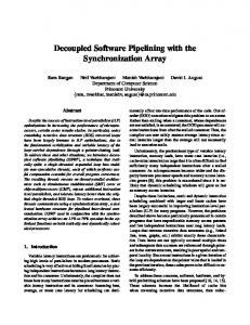
period 2 is stable. Figure 1 shows the absolute value of the maximum eigenvalue, 兩 ␭ max 兩 , as a function of ⑀ , for an array of N⫽12 maps and three different values of the parameter a. For a⫽3.5 共dot-dashed line兲, the maps without coupling evolve in a limit cycle of period 4; for a⫽3.83 共dashed line兲, the maps without coupling evolve in a limit cycle of period 3; and for a⫽4 共solid line兲, the maps without coupling are chaotic. For clarity, the dotted line indicates the stability boundary 兩 ␭ max 兩 ⫽1. In the three cases, for large enough coupling the antiphase solution of period 2 is stable 共兩␭max兩⬍1兲. Notice that the coupling strength above which the solution is stable increases with increasing a. We verified numerically that for larger arrays, the antiphase solution is stable. Figure 2共a兲 displays, as an example, a bifurcation diagram for N⫽50 (a⫽4 and k⫽1). The bifurcation diagram is done in the following way: we chose the same initial condition for all values of ⑀ , and we plot the 100 time-consecutive values x i (t) 共with t large enough兲 for a given element i of the array. Figure 2共b兲 displays the same but for a neighboring element. Above a certain coupling strength, the array synchronizes in the period-2 orbit of the uncoupled map, and the bifurcation diagram for the two elements coincide. The synchronization in the period-2 orbit is surprising since for a⫽4, the period-2 orbit

056219-3

A. C. MARTI´ AND C. MASOLLER

PHYSICAL REVIEW E 67, 056219 共2003兲

FIG. 1. Stability analysis of the antiphase solution of period 2 for k⫽1 and N⫽12. We plot the largest eigenvalue of the matrix A 关Eq. 共17兲兴 vs the coupling strength for a⫽3.5 共dot-dashed line兲, a ⫽3.83 共dashed line兲, and a⫽4 共solid line兲.

is unstable for the uncoupled maps. While the antiphase solution is stable for ⑀ ⭓0.6 共see Fig. 1兲, Fig. 2 shows that the array synchronizes in this solution for a slightly larger coupling strength ( ⑀ ⬃0.7). The critical coupling strength ⑀ crit , above which global synchronization occurs, depends slightly on the initial condition, and increases with increasing a and N. Figure 3 displays the critical value of ⑀ 共calculated averaging over 100 different initial conditions兲 vs a. ⑀ crit increases linearly in the parameter region where the uncoupled maps are periodic, and abruptly in the parameter region where the uncoupled maps are chaotic. Figure 4 共solid line兲 shows that ⑀ crit also increases with increasing system size N. Notice that below the critical coupling strength ⑀ crit , the bifurcation diagrams shown in Figs. 2共a兲 and 2共b兲 differ. This is due to the fact that for ⑀ ⬍ ⑀ crit , the array splits into a complex clustered structure. The clustering behavior in the simpler case where the uncoupled maps evolve in a period-2 orbit was studied in Ref. 关14兴. For larger time delays and k odd, the interval of coupling strength in which the antiphase solution of period 2 is stable becomes more narrow. As an example, Fig. 5 displays 兩 ␭ max 兩

FIG. 2. Bifurcation diagram obtained numerically, integrating Eq. 共3兲 with a⫽4, k⫽1, and N⫽50. We plot the values of two consecutive elements, x i 共a兲 and x i⫹1 共b兲. Notice that after a complex bifurcation scenario, the two elements of the array synchronize in a period-2 orbit.

FIG. 3. Critical coupling strength above which synchronization occurs vs the nonlinear parameter a. k⫽1 and N⫽100. ⑀ crit was calculated averaging over 100 different initial conditions.

vs ⑀ for a⫽3.5 and k⫽1,3,5, and 7. Note that in a wide range of coupling strength, 兩 ␭ max 兩 is slightly larger than 1. In this parameter region, starting from random initial conditions there is a transient time in which the array approaches the antiphase solution; after this transient the array exhibits a complex spatiotemporal behavior. The transient time increases with N; as an example, Fig. 6 displays the mean N x i vs time, for four different system sizes. value 具 x 典 ⫽ 兺 i⫽1 The study of this unexpected effect of the system size is the object of future work. Next, we show results for the in-phase solution, which exists for k⫽n P. Figure 7 displays the bifurcation diagram for two elements of the array, and a⫽3.5, k⫽4, and N ⫽50 共for a⫽3.5, the uncoupled maps evolve in an orbit of period 4兲. We observe that above a critical coupling strength ( ⑀ crit ⬃0.23), the array synchronizes in the period-4 orbit of

FIG. 4. Critical coupling strength above which global synchronization occurs as a function of N for a⫽3.5 and k⫽1 共solid line兲; a⫽3.5 and k⫽4 共dashed line兲.

056219-4

PHYSICAL REVIEW E 67, 056219 共2003兲

DELAY-INDUCED SYNCHRONIZATION PHENOMENA IN . . .

FIG. 7. Bifurcation diagram obtained numerically, integrating Eq. 共3兲 with a⫽3.5, k⫽4, and N⫽50. We plot the values of two different elements of the array, x i 共a兲 and x j 共b兲. Notice that after a period-halving bifurcation, the elements of the array synchronize in a period-4 orbit. IV. SUMMARY AND CONCLUSIONS

FIG. 6. Temporal evolution of the mean value 具 x i (t) 典 for four different system sizes, N⫽12 共a兲, N⫽30 共b兲, N⫽50 共c兲, and N ⫽80 共d兲. The parameters are a⫽3.5, k⫽5, and ⑀ ⫽0.6

We studied the synchronization of a linear array of identical logistic maps. We consider time-delayed mutual coupling with delay times ␶ i j that are proportional to the distance between the maps ( ␶ i j ⫽k 兩 i⫺ j 兩 ). Depending on the time delays and on the coupling strength, different synchronization regimes might occur. If the coupling is weak, the array usually splits into a complex clustered structure. If the coupling is large enough, global synchronization occurs. In the globally synchronized state, each element of the array sees all other elements in its present state 关 x i (t)⫽x j (t ⫺ ␶ i j ) ᭙i, j], and all the elements of the array evolve along a periodic orbit of the uncoupled maps. The spatial correlation along the array is either periodic or homogeneous depending on k. If k is odd, the array synchronizes in antiphase, such that the state at time t of two consecutive elements is x i (t) ⫽x 0 (t), x i⫹1 (t)⫽x 0 (t⫹ P/2) 关where x 0 (t) is a particular realization of the orbit of period P, used as a reference兴. If k⫽n P, the array synchronizes in phase, such that the state at time t is x i (t)⫽x 0 (t) ᭙ i. For parameter values such that the uncoupled maps are chaotic, mutual delayed coupling suppresses chaos, rendering the evolution of the elements of the array periodic in time. Thus, an important consequence of our analysis is that delayed coupling might allow controlling an assembly of chaotic maps by rending an unstable periodic orbit of the uncoupled maps, stable. In addition, the antiphase synchronization regime found here might be of interest in the context of population models 关15–17兴 where an increase of the connectivity among isolated populations leads to in-phase synchronization of local population oscillations and thereby increases the danger of global extinction. Our results suggest that if a distant-dependent delay is taken into account, under appropriate conditions an increase of the connectivity might lead to coherent antiphase oscillations of the local populations, thus avoiding the danger of global extinction.

关1兴 A.S. Pikovsky, M.G. Rosenblum, and J. Kurths, Synchronization—A Universal Concept in Nonlinear Sciences 共Cambridge University Press, Cambridge, 2001兲.

关2兴 S. Boccaletti, J. Kurths, G. Osipov, D.L. Valladares, and C.S. Zhou, Phys. Rep. 366, 1 共2002兲. 关3兴 K. Kaneko, Phys. Rev. Lett. 63, 219 共1989兲.

FIG. 5. Modulus of the largest eigenvalue of the matrix A as a function of ⑀ for the antiphase solution and a⫽3.5, k⫽1 共o兲, k ⫽3 共x兲, k⫽5 (*), and k⫽7 (⫹).

the uncoupled map. As in the case of the antiphase solution, for coupling strengths below ⑀ crit , the bifurcation diagrams shown in Figs. 7共a兲 and 7共b兲 differ. This is due to the fact that the two elements belong to different clusters. The dashed line in Fig. 4 shows that ⑀ crit increases with increasing system size N. For arbitrary values of k, a, and ⑀ , we found a rich variety of complex spatiotemporal behaviors. The characterization of the different dynamic regimes is the object of future work.

056219-5

A. C. MARTI´ AND C. MASOLLER

PHYSICAL REVIEW E 67, 056219 共2003兲

关4兴 K. Kaneko, Physica D 41, 137 共1990兲. 关5兴 A. Pikovsky, O. Popovych, and Y. Maistrenko, Phys. Rev. Lett. 87, 044102 共2001兲. 关6兴 O. Popovych, A. Pikovsky, and Yu. Maistrenko, Physica D 168-169, 106 共2002兲. 关7兴 J. Garcia-Ojalvo, J. Casademont, C.R. Mirasso, M.C. Torrent, and J.M. Sancho, Int. J. Bifurcation Chaos Appl. Sci. Eng. 9, 2225 共1999兲. 关8兴 G. Kozyreff, A.G. Vladimirov, and P. Mandel, Phys. Rev. Lett. 85, 3809 共2000兲. 关9兴 Y. Jiang, Phys. Lett. A 267, 342 共2000兲. 关10兴 P. Parmananda, M. Hildebrand, and M. Eiswirth, Phys. Rev. E

56, 239 共1997兲. 关11兴 P.M. Gade, Phys. Rev. E 57, 7309 共1998兲. 关12兴 D.H. Zanette, Phys. Rev. E 62, 3167 共2000兲. 关13兴 S.O. Jeong, T.W. Ko, and H.T. Moon, Phys. Rev. Lett. 89, 154104 共2002兲. 关14兴 C. Masoller, A.C. Martı´, and D. Zanette 共unpublished兲. 关15兴 A. Hastings, Ecology 74, 1362 共1993兲. 关16兴 B. Blasius, A. Huppert, and L. Stone, Nature 共London兲 399, 354 共1999兲. 关17兴 D.J.D. Earn, S.A. Levin, and P. Rohani, Science 共Washington, DC, U.S.兲 290, 1360 共2000兲.

056219-6