Density functional theory for a model colloid–polymer mixture: bulk

INSTITUTE OF PHYSICS PUBLISHING

JOURNAL OF PHYSICS: CONDENSED MATTER

J. Phys.: Condens. Matter 14 (2002) 9353–9382

PII: S0953-8984(02)35570-X

Density functional theory for a model colloid–polymer mixture: bulk fluid phases Matthias Schmidt1 , Hartmut Löwen1 , Joseph M Brader2,3 and Robert Evans2 1

Institut für Theoretische Physik II, Heinrich-Heine-Universität Düsseldorf, Universitätsstraße 1, D-40225 Düsseldorf, Germany 2 H H Wills Physics Laboratory, University of Bristol, Royal Fort, Tyndall Avenue, Bristol BS8 1TL, UK

Received 10 April 2002, in final form 18 June 2002 Published 27 September 2002 Online at stacks.iop.org/JPhysCM/14/9353 Abstract We describe a density functional theory for mixtures of hard sphere (HS) colloids and ideal polymers, the Asakura–Oosawa model. The geometrybased fundamental measures approach which is used to construct the functional ensures the correct behaviour in the limit of low density of both species and in the zero-dimensional limit of a cavity which can contain at most one HS. Dimensional crossover is discussed in detail. Emphasis is placed on the properties of homogeneous (bulk) fluid phases. We show that the present functional yields the same free energy and, therefore, the same fluid–fluid demixing transition as that given by a different approach, namely the freevolume theory. The pair direct correlation functions ci(2) j (r ) of the bulk mixture are given analytically. We investigate the partial structure factors Si j (k) and the asymptotic decay, r → ∞, of the total pair correlation functions h i j (r ) obtained from the Ornstein–Zernike route. The locus in the phase diagram of the crossover from monotonic to oscillatory decay of correlations is calculated for several size ratios q = R p /Rc , where R p is the radius of the polymer sphere and Rc that of the colloid. We determine the (mean-field) behaviour of the partial structure factors on approaching the fluid–fluid critical (consolute) point.

1. Introduction This paper describes a density functional theory (DFT) for determining the equilibrium properties of the so-called Asakura–Oosawa (AO) model of colloid–polymer mixtures [1, 2]. The model, which was first written down by Vrij [2], treats the colloids as hard spheres (HS) and the globular polymer coils as interpenetrating spheres, as regards their mutual interactions, 3

Present address: James Franck Institute, University of Chicago, South Ellis Ave. 5640, Chicago, IL 60637, USA.

0953-8984/02/409353+30$30.00

© 2002 IOP Publishing Ltd

Printed in the UK

9353

9354

M Schmidt et al

but polymers experience an excluded volume (hard) interaction with the colloids. It can be regarded as the simplest, zeroth-order, model of a mixture of colloidal particles and nonadsorbing polymers. Much attention has been paid to the bulk properties of the AO model since this affords an important example of pure entropy-driven fluid–fluid phase separation. When q, the size ratio of the radius of the polymer sphere to that of the colloid sphere, is sufficiently large, the mixture separates into colloid-rich (liquid) and colloid-poor (gas) phases. The earliest detailed theoretical treatment of the model was that by Gast et al [3] based on liquid state perturbation theory for the (approximate) one-component version where colloids are assumed to interact via the AO pair potential. An alternative approach was introduced by Lekkerkerker et al [4] based on a free-volume theory for the free energy of the mixture—see section 3.1. These approximate theories, along with some simulation studies of simplified versions of the AO model [5, 6], indicate that when the size ratio q is larger than about 0.35 fluid–fluid separation is stable with respect to the fluid–solid transition. Other studies have investigated the equilibrium pair correlation functions in the AO model [5, 7–9] and the formal status of the mapping to a one-component fluid [8]. Although the AO model is highly idealized the variation of bulk phase behaviour with q predicted by studies of the model is in keeping with the experimental results [10, 11]. More recently attention has shifted towards inhomogeneous mixtures. An effective Hamiltonian for the colloids was obtained by integrating out the degrees of freedom of√the polymer with both species subject to external fields [12, 13]. When the size ratio q < (2/ 3 −1) = 0.1547 . . . the effective Hamiltonian contains only one- and two-body (pairwise) contributions and for such mixtures it is straightforward to apply this to problems of adsorption at a hard wall [13]. For larger size ratios many-body terms are present in the effective Hamiltonian for both bulk and inhomogeneous mixtures [5, 8, 13] and incorporating such terms is rather complicated. Thus treating fluid–fluid interfaces and adsorption phenomena which occur for larger values of q is difficult within the effective Hamiltonian perspective and ad hoc prescriptions have been made [12] in order to calculate the density profile of colloids and the surface tension of the free fluid–fluid interface and compare with experimental data [14, 15]. The approach we adopt here for the AO model does not exploit the formal mapping to an effective one-component system of colloids. Rather we treat colloid and polymer on equal footing and develop a DFT specifically tailored for the AO mixture. DFT is recognized as powerful tool for describing the equilibrium properties of inhomogeneous fluids [16, 17]. Most effort has been expended on HS fluids, and the fundamental measure theory (FMT) introduced by Rosenfeld [18] and subsequently refined [19–22] has proved particularly versatile and reliable in a wide variety of applications to both pure HS and to mixtures. The FMT approach has also been applied to parallel hard cubes [23, 24]. Other recent advances in geometry-based DFT include (i) penetrable spheres [25], where the interatomic potential is a finite constant when the separation is smaller than the sphere diameter, (ii) the Widom–Rowlinson model [26], where the unlike species interact via a hard core potential and the like–like interactions are ideal, (iii) a model proposed by Bolhuis and Frenkel [27] that describes a mixture of HS and infinitely thin needles [28], (iv) a model of an amphiphilic hard body mixture [29] and (v) a ternary mixture of colloids, polymers and needles [30]. Our DFT for the AO model is also based on FMT ideas. An earlier letter [31] gave a brief outline of the theory and some results for bulk properties while a second letter described applications to fluid–fluid interfaces and wetting behaviour for the mixture adsorbed at a hard wall [32]. In this paper we provide a comprehensive description of the functional and its bulk properties

Density functional theory for a model colloid–polymer mixture: bulk fluid phases

9355

(thermodynamic functions and pair correlation functions) which explains the status of the DFT and which lists explicit expressions for all the relevant quantities required to implement the formalism. Detailed results for interfacial properties obtained from the DFT are given in [9]. Our paper is organized as follows: section 2 is devoted to the theory. We begin in 2.1 with an overview of DFT and describe the strategy for constructing functionals based on the FMT approach. The AO model is specified in 2.2 and in 2.3 we examine two exact limiting cases, namely the low density expansion and the zero-dimensional limit which corresponds to a small cavity that can hold at most one colloidal sphere. The free energy of the latter case constitutes a generating function for the three-dimensional functional and this is described in 2.4 where the functional for the AO model is presented explicitly. Section 2.5 focuses on the properties of the functional in various limiting cases and, in particular, how it accounts for zero-, one- and two-dimensional density distributions. An alternative derivation of the functional is presented in section 2.6. This is based on the original binary HS functional of Rosenfeld [18] and some observations on the diagrammatic expansions of the pair direct correlation functions for HS and for the AO model. We comment on the procedure of integrating out polymer degrees of freedom in the context of DFT and the nature of an effective one-component functional in 2.7. Section 3 is concerned with the predictions of the DFT for the properties of homogeneous (bulk) fluid phases. In 3.1 we focus on thermodynamic functions and show that the bulk free energy of the mixture is precisely the same as that obtained from the free-volume theory of Lekkerkerker et al [4]. Fluid–fluid demixing is described in 3.2 where it is shown that the spinodal in the ηp , ηc plane can be obtained analytically. ηp , ηc refer to the packing fractions of polymer and colloid, respectively. Section 3.3 describes the pair direct correlation functions ci(2) j (r ) obtained by functional differentiation of our AO functional; these are given analytically and their behaviour with ηp and ηc is discussed. In 3.4 we focus on the partial structure factors Si j (k) of the AO mixture and their behaviour when the mixture is close to the consolute (critical) point. Since the Si j (k) are given analytically the correlation length of the bulk fluid can be extracted straightforwardly. Section 3.5 is concerned with the nature of the asymptotic decay of pair correlations in the bulk AO mixture. We present results for the so-called Fisher– Widom (FW) line, which denotes the line in the phase diagram where the ultimate decay of the total pair correlation functions h i j (r ) crosses over from monotonic to oscillatory. Section 3.6 discusses the predictions of the present DFT for the effective interaction (depletion potential) between colloidal particles, contrasting the Ornstein–Zernike (OZ) route with the alternative test-particle route. We conclude in section 4 with a summary and a discussion of some of the advantages and some shortcomings of our approach. 2. Theory 2.1. Overview and strategy Within DFT the basic variables that describe the microscopic degrees of freedom of a manybody system are the one-body densities ρi (r ) of each species i : ρi (r ) dV is the average number of particles (of species i ) in an infinitesimal volume element dV located at position r . Clearly ρi (r ) can resolve inhomogeneities (spatial deviations from a uniform value) on small length scales. Such inhomogeneous structuring is present in liquids under external influence ( j) and is manifestly present in crystalline solids. Introducing the particle positions ri , where j = 1, . . . , Ni , and Ni is the total number of particles of species i , one defines Ni ( j) ρi (r ) = δ(r − ri ) , (1) j =1

9356

M Schmidt et al

where the angular brackets denote an appropriate ensemble average over many configurations. Evidently the ρi (r ) for a given statepoint (e.g. temperature and chemical potentials µi ) contain considerable knowledge about the system. More significant is the fact that the thermodynamic potential of the system is determined solely by the one-body densities. The existence of a functional that converts the functions ρi (r ) to the grand potential (which is a number) is one of the building blocks of DFT. Within this description, the ρi (r ) are basically the system’s only degrees of freedom. At first glance this may seem to be a limitation: how can the important structural information contained in higher-body correlations such as the pair distribution functions be obtained, if the theory operates on the one-body level? The answer lies in the second building block of DFT: the variational principle states that upon varying the ρi (r ), the grand potential functional is a minimum at the true equilibrium densities and its value at the minimum is the true grand potential . The grand potential functional has the form [ρi (r )] = Fexc [{ρi (r )}] + Fid [ρi (r )] + d3r ρi (r )[Vi,ext (r ) − µi ], (2)

i

− 1] is the (Helmholtz) free energy of the where Fid [ρi (r )] = kB T d r ideal gas, kB is Boltzmann’s constant, T is temperature, i is the thermal wavelength of species i and Vi,ext is an external potential acting on species i . Fexc is the excess Helmholtz free energy arising from interactions between the particles. As this formalism is an exact reformulation of equilibrium statistical mechanics, the hierarchy of higher-body direct correlation functions can be obtained by functional differentiation of Fexc with respect to the density fields and the equilibrium distribution functions from the OZ equation. The main benefit of DFT is that powerful approximate theories can be obtained, provided the (generally unknown) excess part Fexc is prescribed. The effects caused by different classes of (time-independent) external potentials can all be treated within the same theory, as Fexc is independent of Vi,ext ; it is a unique functional of {ρi (r )} for a given choice of interparticle potential functions [16, 17]. Of course, the difficult part of any approximate DFT is finding a suitable prescription or recipe for Fexc that will incorporate the essential physics of short-range correlations (arising from the packing of the particles) and of attractive forces (if these are present) between the particles. However, in all cases, Fexc contains non-local contributions: when varying the density at a given point in space, the system is affected on the length scale of the inter-particle potentials (and beyond that through mediated correlations). Our present DFT recipe to convert colloid and polymer density profiles to an (approximate) excess free energy for the AO model has the following key features. The non-local character is taken care of by convoluting the actual density fields ρi (r ) with various weight functions. The results of this procedure are weighted densities, and only these are subsequently used to obtain the excess free-energy functional, not the bare density fields. This type of weighteddensity approximation (WDA) is now the most common tool to deal with very pronounced inhomogeneities: bare density profiles may change by orders of magnitude over distances as small as a particle diameter [33] and convolutions are a suitable means of treating this behaviour as they exhibit the property of smoothing out. Extensitivity of the free energy is incorporated by expressing Fexc as a spatial integral over an excess free-energy density . This ensures that, over length scales which are large compared with the system’s correlation lengths, distinct regions of space give additive contributions to the free energy. In order to connect the free-energy density with the weighted densities, our crucial approximation is to regard as a simple function (not a functional) of the weighted densities. This feature of the theory is identical to that of Rosenfeld’s HS functional [18], and to various recent DFTs mentioned in the introduction. The three main differences between this approach and most other weighted-density [16, 17] DFTs are the following. 3

ρi (r )[ln(3i ρi (r ))


9357

(i) Rather than a single weight function, we use a set of weight functions wνi (labelled by ν) for each species i . Consequently, we have a set of weighted densities n iν for each species i . (ii) The range of the weight functions (defined as the distance beyond which a weight function vanishes) is determined not by the range of interactions, but by the radii of the particles. (iii) The free-energy density is not modelled as a product of a bare density times a free energy per particle, but as a function only of the weighted densities n iν . Our DFT is constructed specifically to describe the AO model, i.e. the forms of the wνi and of are specific to this model. These are obtained by imposing the correct behaviour of the functional in several different cases, where the exact behaviour of the AO model is known. The low density (virial) expansion enables us to obtain the explicit form of the weight functions. As we shall see below, these are the same as for HS [18]. The other case is a situation of extreme confinement, where the particles of the system are only allowed to access a single location in space. This zero-dimensional limit is reminiscent of confining a particle to a crystal lattice site and corresponds to imposing the density distribution for a particle in a small cavity whose dimensions are of the same size as the particle. For HS the importance of this limit was demonstrated by Rosenfeld et al [19, 20]. Later it was shown that the original Rosenfeld functional [18], as well as improved versions, can be obtained from a systematic treatment of superpositions of (up to three) such density peaks [21, 22]. 2.2. Specification of the Asakura–Oosawa model The AO model describes colloids as hard impenetrable spheres and polymers as effective particles with spherical shape. These polymeric spheres are ideal (non-interacting) amongst themselves, but experience a hard core repulsion with the colloids. Clearly, the model is idealized, but it captures the essential physics of real colloid–polymer mixtures. In particular, the AO model describes polymer coils at the theta point, where repulsion is balanced by attraction, such that the effective interaction between polymers (as expressed by their second virial coefficient) vanishes. The AO model should also be regarded as a useful zeroth-order reference system for a wide variety of complex fluids where soft penetrable particles move in the space between hard bodies. Thus, we consider a mixture of Nc colloids with radii Rc , and Np polymers, with radii Rp , interacting via pair potentials Vi j , with i, j = c, p, contained inside a (large) volume V . The Hamiltonian consists of (trivial) kinetic energy terms and a sum of interaction terms: H ({Ri , r j }) =

Nc i< j

Vcc (|Ri − R j |) +

Np Nc i

Vcp (|Ri − r j |) +

j

Np

Vpp (|ri − r j |),

(3)

i< j (p)

where {Ri } = {ri(c) } denotes colloid and {ri } = {ri } polymer coordinates. The interaction potential between colloids is hard: Vcc (r ) = ∞ if r 2Rc , and zero otherwise. The interaction between colloids and polymers is also hard: Vcp (r ) = ∞, if r Rc + Rp , and zero otherwise. The interaction between polymers vanishes for all distances [2]: Vpp (r ) = 0. Since all the interactions between particles are either hard or ideal, temperature T plays no role in determining phase behaviour or structure and the thermodynamic state of the bulk system is governed by the packing fractions of colloids, ηc = 4π Nc Rc3 /(3V ), and of polymers, ηp = 4π Np Rp3 /(3V ). The properties of the system are governed by the size ratio q = Rp /Rc , which is the only adjustable parameter in the model. Unlike other theoretical treatments which are based on some integrating out of polymer degrees of freedom [3–5, 12, 13] the present DFT of the AO model treats colloid and polymer on equal footing.

9358

M Schmidt et al

2.3. Two exact limiting cases 2.3.1. Low density expansion. For small densities of all species, ρi → 0, the probability that particles interact is small and for uniform fluids this enables one to make the systematic virial expansion of thermodynamic functions in powers of the (bulk) densities. The lowest order term governs density behaviour and for the excess free energy this is simply the low β Fexc /V = − i j ρi ρ j d3r f i j (r )/2, where f i j (r ) = exp(−βVi j (r )) − 1 are the Mayer functions, with β = 1/kB T , and the summations run over all species. A similar expansion can be performed for inhomogeneous systems [16–18]. For a mixture the lowest-order term is 1 (4) d3r d3r ρi (r ) f i j (|r − r |)ρ j (r ). β Fexc [{ρi (r )}] = − 2 ij

Note that as the AO model exhibits only hard core interactions, the f i j take on the values −1 and 0 only: fcc , f cp = −1 if the particle pair overlaps, and are zero otherwise. f pp = 0 for all separations r . Equation (4) sums double convolutions of the density profiles, where the Mayer function is the convolution kernel. Although the functional is only second order in densities, an important feature is already present: the range of non-locality is the range of interactions. 2.3.2. Zero-dimensional limit. In statistical physics it is a common simplification to consider models in reduced spatial dimensionality d. Often two-dimensional systems are simpler to tackle than three-dimensional systems, and one-dimensional systems are usually simpler than two-dimensional systems. Reduced dimensionalities not only simplify theoretical treatments, but are also realized in nature, e.g. in films (two dimensions) or inside channels (one dimension) or cavities (zero dimensions). A versatile DFT should be able to describe accurately all situations of reduced dimensionality. In order to model the ultimate dimensional crossover to zero dimensions a special limit was introduced [19, 20]. In this so-called zero-dimensional limit the system is confined in all three spatial dimensions, such that only a single point in three-dimensional space is accessible for the particles. Physically, the zero-dimensional limit may be realized by a small cavity with rigid walls, that is of particle size. The zerodimensional limit is also similar to that of a particle at a crystal lattice site, where each particle is confined within the cage of its nearest neighbours. Any theoretical description for structure and thermodynamics in highly inhomogeneous three-dimensional situations should be able to reproduce dimensional crossover, even to the extreme limit of a zero-dimensional situation. Clearly, this is a demanding requirement. It has been found, in the case of HS, that one can start with a point and by considering zero-dimensional cavities of increasingly complex shape build up a theory for higher dimensions. A strong guide for the general structure of the functional is provided by Percus’s exact one-dimensional functional for hard rods [34]. In the case of HS knowledge of the exact zero-dimensional free energy was sufficient to derive a working theory [21], and was subsequently exploited to derive improved versions [22]. The same methodology was used to tackle other systems including penetrable spheres, which interact with a constant pair potential if they overlap [25], the Widom–Rowlinson model [26] and a needle–sphere mixture [28], as well as models for an amphiphilic [29] and a ternary mixture [30]. Here we follow the same route for the AO model. To be explicit, we introduce an external potential Vext (r ) = 0 if |r | < , and ∞ otherwise. Each particle’s centre is then allowed to move inside a sphere of volume 4π 3 /3. We consider the limit → 0, so that any particles present in the cavity overlap. In order to derive the zero-dimensional Helmholtz (excess) free energy, we consider the grand partition sum . The only states that are allowed are the following: (i) the empty state without any particle,


9359

(ii) the state with exactly one colloidal particle and (iii) all states without colloids but with an arbitrary number of polymers. Hence, in that order, = 1 + z c + [exp(z p ) − 1] = z c + exp(z p ),

(5)

3 where the (dimensionless) fugacities are defined here as z i = exp(βµi )−3 i 4π /3. The mean occupation numbers of particles, ηi , which are the packing fractions in zero dimension, are obtained from ∂ ηi = z i ln . (6) ∂z i More explicitly, zc ηc = , (7) z c + exp(z p ) z p exp(z p ) ηp = , (8) z c + exp(z p )

which can be inverted to obtain the fugacities ηp ηc exp zc = , 1 − ηc 1 − ηc ηp . zp = 1 − ηc The dimensionless excess chemical potentials, µ˜ i ≡ ln(z i ) − ln(ηi ), given by ηp µ˜ c (ηc , ηp ) = − ln(1 − ηc ) + , 1 − ηc µ˜ p (ηc ) = − ln(1 − ηc ),

(9) (10)

(11) (12)

can then be used to integrate along a suitably chosen path in the (ηc , ηp ) plane in order to obtain the excess free energy ηc ηp β F0d (ηc , ηp ) = dηc µ˜ c (ηc , 0) + dη µ˜ p (ηc ). (13) 0

0

(Alternatively, one could use β F0d = − ln + µ˜ c ∂ ln /∂ µ˜ c + µ˜ p ∂ ln /∂ µ˜ p .) The result is β F0d (ηc , ηp ) = (1 − ηc − ηp ) ln(1 − ηc ) + ηc .

(14)

This zero-dimensional free energy exhibits a number of physically realistic properties, that are generic to the model itself, independent of the precise situation under consideration, and which remain valid for other reduced dimensionalities and confining geometries: (i) The colloid packing fraction is restricted to ηc < 1. In three dimensions, ηc → 1 corresponds to space-filling spheres. Although it is impossible to pack HS more densely than the close-packing fcc value of 0.7405, the limit ηc → 1 does arise in many liquid state approximations such as scaled-particle and Percus–Yevick (PY) theories which commonly produce expressions containing factors of 1/(1 − ηc ). (ii) Polymer packing fractions can be arbitrarily large, as no upper bound exists for ηp ; the ideality of the polymers means that there are no packing constraints for this species. (iii) The free energy depends linearly on ηp . As we shall show in section 2.6, this is not necessarily the case in three-dimensional bulk where terms of O(ηp4 ) and higher, but not O(ηp2 ) or O(ηp3 ), can arise. However, this simple linear dependence is a feature of the well known (approximate) free-volume theory [4, 5].

9360

M Schmidt et al

Additionally, it is interesting to compare the present result for the AO model with the result for HS mixtures. For a binary HS mixture of species 1 and 2, one obtains bhs = (1 − η1 − η2 ) ln(1 − η1 − η2 ) + η1 + η2 , where η1 , η2 are the packing fractions of β F0d species 1 and 2. Guided by (iii), we observe that linearization in η2 yields F0d of equation (14) upon identifying η1 = ηc and η2 = ηp . This linearization property will be exploited further in section 2.6 in an alternative derivation of the DFT. These two exact limiting cases provide the key building blocks for constructing the freeenergy functional. 2.4. Density functional for the AO model Following previous work on HS mixtures [18–20], we express the excess Helmholtz free energy in terms of a functional of colloid and polymer density fields as a spatial integral over a free-energy density that is a function of the weighted densities: (15) β Fexc [ρc (r ), ρp (r )] = d3 x ({n cν (x)}, {n pγ (x)}), where the weighted densities for each species i = c, p are obtained by convolutions with the actual density profiles i n ν (x) = d3r ρi (r )wνi (x − r ). (16) In previous work on HS, was taken to be a function of species-independent weighted densities [18]. Here we must generalize and allow to depend on species-dependent weighted densities. This is necessary in order to capture the intrinsically different nature of colloids and polymers. The weight functions wνi are independent of the density profiles and are given by w3i (r ) = (Ri − r ),

(17)

w2i (r ) = δ(Ri − r ), w1i (r ) = δ(Ri − r )/(4πr ), w0i (r ) = δ(Ri − r )/(4πr 2 ), i wv2 (r ) = δ(Ri − r )r /r, i wv1 (r ) = δ(Ri − r )r /(4πr 2 ), i ˆ wˆ m2 (r ) = δ(Ri − r )(rr /r 2 − 1/3),

(18) (19) (20) (21) (22) (23)

where r = |r |, (r ) is the step function, δ(r ) is the Dirac distribution and 1ˆ is the identity matrix. The weight functions are quantities with dimension length 3−ν . They differ in their i i i tensorial rank: w0i , w1i , w2i , w3i are scalars; wv1 , wv2 are vectors; wˆ m2 is a (traceless) secondrank tensor. Equations (17)–(22) are the weights given in [18], whereas equation (23) is equivalent to the tensor formulation in [22]. The Fourier transforms of the weight functions are given in appendix A. The free-energy density is composed of three parts = 1 + 2 + 3 ,

(24)

which are defined as p 1 = n i0 ϕi (n c3 , n 3 ),

(25)

i=c,p

2 =

j

j

p

(n i1 n 2 − niv1 · nv2 )ϕi j (n c3 , n 3 ),

i, j =c,p

(26)


9361

1 1 i j k 3 i j k p j i j k i k n n n − n 2 nv2 · nv2 + nv2 nˆ m2 nv2 − tr(nˆ m2 nˆ m2 nˆ m2 ) ϕi j k (n c3 , n 3 ), 3 = 8π i, j,k=c,p 3 2 2 2 2 (27) where tr denotes the trace, and derivatives of the zero-dimensional excess free energy (given by equation (14)) are ∂m ϕi...k (ηc , ηp ) ≡ β F0d (ηc , ηp ). (28) ∂ηi . . . ∂ηk In the absence of polymer, 1 and 2 are equivalent to the free-energy densities for HS introduced in [18], and 3 is equivalent to the tensor treatment for pure HS in [22]. Equations (25)–(27) are direct generalizations of these earlier treatments to include summation over species. All the derivatives ϕi... j that carry more than one polymer index vanish due to the functional form of F0d , and we obtain p n3 p c c 1 = n 0 − ln(1 − n 3 ) + (29) − n 0 ln(1 − n c3 ), 1 − n c3 p p p p p n 1 n c2 − nv1 · ncv2 + n c1 n 2 − ncv1 · nv2 n3 1 + + , (30) 2 = (n c1 n c2 − ncv1 · ncv2 ) 1 − n c3 (1 − n c3 )2 1 − n c3 p 1 c 3 c c (n ) − n c2 (ncv2 )2 + 23 (ncv2 nˆ m2 ncv2 − 3 det nˆ m2 ) 2n 3 1 3 2 + 3 = 8π (1 − n c3 )2 (1 − n c3 )3 p

+

p

p

p

p

p

c c 2 (n c2 )2 n 2 − n 2 (ncv2 )2 − 2n c2 ncv2 · nv2 + 32 {2nv2 nˆ m2 ncv2 + ncv2 nˆ m2 ncv2 − 3tr[(nˆ m2 ) nˆ m2 ]}

8π(1 − n c3 )2

.

(31) For brevity we have omitted the r dependence, e.g. = The DFT for the AO model is now fully specified. In the next subsection we examine several limiting cases in order to ascertain better the nature of the approximation we have introduced. n c3

n c3 (r ).

2.5. Examining limiting cases of the functional 2.5.1. Low density expansion. For low densities, ρi → 0, the weighted densities also become small, n iν → 0, since the latter are given by a convolution of the density with a density-independent weight function wνi , equation (16). In order to obtain the behaviour of the DF, we Taylor expand the free-energy density in powers of weighted densities. The straightforward calculation yields to lowest order p

p

p

p

p

p

= n c0 n c3 + n c1 n c2 − ncv1 · ncv2 + n c0 n 3 + n c1 n 2 − ncv1 · nv2 + n 0 n c3 + n 1 n c2 − nv1 · ncv2 .

(32)

j

Each of the terms in the sum is a bilinear combination of weighted densities, n iν n λ . We rewrite this formally as ij j Cνλ n iν n λ (33) ≡ i j =cp νλ

ij

pp

where the coefficients take on values Cνλ = −1, 0, 1. (Note that the coefficients Cνλ of terms p p n ν n λ , with p representing species 2, which are non-zero in the corresponding expansion for the binary HS functional vanish in the AO model.) Next we rearrange the order of integrations in the density functional ij j 3 3 i Cνλ d r ρi (r )wν (r − x) d3r ρ j (r )wλ (r − x) (34) β Fexc = d x i j νλ

9362

M Schmidt et al

=

d3r ρi (r )

ij

=

d3r ρi (r )

d 3 r ρ j (r )

νλ

d 3 x Cνλ wνi (r − x)wλ (r − x) ij

j

d3r ρ j (r ) f i j (|r − r |)/2,

(35) (36)

ij

where in the last step we exploited the property of the weight functions to obtain the HS Mayer bond. This is the same argument as in Rosenfeld’s HS mixture case [18]; the vanishing of the polymer–polymer Mayer bond is due solely to the functional form of , which does not contain terms quadratic in polymer weighted densities. Thus the present functional does reduce to the correct low density limit when all densities ρi → 0. 2.5.2. Zero-dimensional limit. For density distributions ρi = ηi δ(r ) each weighted density becomes proportional to its weight function (37) n iν (x) = d3r ηi δ(r )wνi (r − x) = ηi wνi (x). We show that the contribution from 1 yields the exact result. Consider β Fexc = d3r 1 ∞ p = dr 4πr 2 ηi w0i (r )ϕi (ηc w3c (r ), ηp w3 (r ))

0

∞

=

dr

0

dr

0

ηi δ(Ri − r )ϕi (ηc (Rc − r ), ηp (Rp − r ))

ηi

i 1

=

(39)

i

(40)

i

∞

=

(38)

−d(Ri − r ) ϕi (ηc (Rc − r ), ηp (Rp − r )) dr

dt[ηp ϕp (ηc , ηp t) + ηc ϕc (ηc t, 0)],

(41) (42)

0

= β F0d (ηc , ηp )

(43)

where we have assumed, without loss of generality, in equation (42) that Rc > Rp and have used the definition of ϕi , equation (28), in the last step. The contributions from 2 and 3 both vanish. This follows from symmetry i considerations. From equation (37), and the fact that wvν = wνi r /r for ν = 1, 2, it follows j i j i that n 1 n 2 = nv1 · nv2 . Hence, from equation (30), 2 = 0. A similar argument holds for 3 . 2.5.3. One-dimensional limit. Following [21] we can obtain an effective one-dimensional functional by imposing on the general three-dimensional functional density distributions ρi (r ) = ρi (x)δ(y)δ(z). We omit the tedious details and show the final result: β Fexc [ρc (x), ρp (x )] = dx ({n cν (x)}, {n pγ (x)}), (44) where the weighted densities are obtained by one-dimensional convolutions i n ν (x) = dx ρi (x )wνi (x − x ),

(45)

of the two one-dimensional weight functions wdi (x) = θ (Ri − |x|),

(46)

w0i (x)

(47)

= [δ(Ri + x) + δ(Ri − x)]/2.


9363

Note that wdi originates from the three-dimensional weight w3i , and describes the onedimensional packing fraction. The excess free-energy density obtained from 1 + 2 , i.e. equations (29), (30), is

p (48) n i0 ϕi n cd , n d = i=c,p p

p

= −(n c0 + n 0 ) ln(1 − n cd ) +

n c0 n d . 1 − n cd

(49)

Note that the remaining term 3 , equation (31), gives an additional contribution if q = 1. Following the discussion of two-dimensional crossover in HS mixtures [35] we expect this contribution to be negligible. We note that the bulk equation of state derived from in equation (49) is the same as that of free-volume theory in one dimension. As the latter is known to yield a very good approximation to the exact solution of the one-dimensional AO model [36], provided the reservoir packing fraction ηp,r is smaller than about 1.5, it is likely that the one-dimensional functional will also be accurate in this regime. To summarize, in this subsection we have shown that our DF for the AO model does yield the correct low density and zero-dimensional limits and that for uniform one-dimensional density distributions the theory is equivalent to free-volume theory. For completeness, a twodimensional functional is presented in appendix B. 2.6. Alternative derivation of the DFT We show here that the present functional (section 2.4) can be derived in an alternative fashion starting from the binary HS functional of Rosenfeld [18]. The only distinction between the AO model and the binary HS model is that the interaction V22 between particles of species 2 is zero. Thus all the necessary geometrical information about sphere packing is already included and it is possible, at least in principle, to extract a functional for the AO model. More precisely, if we had the exact functional for the binary HS model then a density expansion would contain all the diagrams required for the AO model plus an additional class of diagrams containing Mayer bonds between polymers. An operation which removes the unwanted class diagrams from the binary HS functional would yield the exact functional for the AO model. In order to extract the information we require from the binary HS functional, we turn to the exact low density diagrammatic expansion of the bulk pair direct correlation function. For the AO model this is given by (2) (r ) = ccc

+ ρc

+ ρp

(2) (r ) ccp (2) (r ) cpp

+ ρc

+ O(ρ )

=

= 0 + O(ρ 2 ),

+ O(ρ 2 ) 2

(50) (51) (52)

where we have given the expansion up to second order (third virial level). As usual each bond between circles represents a Mayer function and a shaded circle an integration over one coordinate. All diagrams involving a polymer–polymer Mayer bond are zero. To third (2) = 0, as all three contributing diagrams contain a polymer–polymer Mayer virial level, cpp (2) are non-zero as there exist diagrams which bond. Higher order terms in the expansion of cpp contribute and yet do not contain polymer–polymer Mayer bonds. For example, at the fourth virial level the diagram (53)

9364

M Schmidt et al

(2) appears and gives a contribution of order ρ 2p to cpp (r ). It should be noted that the Percus– (2) Yevick theory for the binary AO model also gives cpp = 0. A theory capable of going beyond (2) the approximation cpp = 0 would have to be accurate to at least the fourth virial level. As even sophisticated integral equation theories are usually exact to only third virial level this is clearly a difficult task. Equations (50)–(52) give no information about how to extract the colloid– polymer functional from the binary HS functional as information about the polymer–polymer interaction does not enter until higher terms in the expansion. However, the facts that (2) is independent of the polymer density field and (i) ccp (2) = 0 suggest that the simplest way to obtain a functional for the AO model is to (ii) cpp linearize the binary HS functional with respect to ρ p (r ). (2) This ensures that the bulk pair correlations are correct to the third virial level, i.e. cpp = (2) −δ 2 β Fexc /δρp (r )δρp (r ) = 0 and ccp = −δ 2 β Fexc /δρc (r )δρp (r ) is independent of the polymer density. The exact AO free-energy functional contains terms linear in ρ p (r ) but not terms in ρ 2p or ρ 3p , as these would lead to inconsistency with the low order diagrams. However, when expanding the binary HS functional in ρ p (r ) we could have chosen to omit the ρ 2p and ρ 3p terms, but retain all higher orders; the low order diagrams exercise no constraint over these higher order contributions. In linearizing the functional we have chosen to set all higher order terms to zero. The justification for this can be found by looking at the exact diagrammatic expansion for a binary mixture to fourth virial level: + ρk + ρk ρl + + + + + + + O(ρ 3 ). (54) ci(2) j (r ) = k

k,l

The Rosenfeld binary HS functional generates bulk ci(2) j identical to those from Percus–Yevick theory. The latter is not exact to fourth virial level as it contains only a subset of the required diagrams: ci(2) + ρk + ρk ρl + + + + O(ρ 3 ). (55) j (r ) = k

k,l

All diagrams in PY theory, equation (55), have a Mayer bond connecting i j . We henceforth refer to diagrams of this category as A class and diagrams with no i j Mayer bond as B class (2) . Retaining quartic and higher order terms when expanding the and focus our attention on cpp Rosenfeld HS functional, only HS A-class diagrams would be included. For the AO model (2) and only B-class diagrams all A-class diagrams are identically zero in the expansion of cpp contribute. Inclusion of quartic or higher order terms in the ρ p expansion of the functional would incorporate only unphysical diagrams. The A-class diagrams required for the AO model are not contained within the original binary HS functional. We conclude that by linearizing the original Rosenfeld HS functional in the polymer density we should obtain a functional which describes the AO model. Indeed when such a linearization is performed we recover i = 0, equations (24)–(31) for the free-energy density but with the tensor weighted densities nˆ m2 since the original Rosenfeld functional does not have tensor weights. 2.7. Effective one-component functional When investigating the statistical mechanics of soft matter systems it is frequently advantageous to integrate out some degrees of freedom in order to obtain effective interactions between the particles of the remaining species. This has proved particularly fruitful for the AO


9365

model of colloid–polymer mixtures where the polymer degrees of freedom could be explicitly integrated out for certain size ratios [5, 8, 9, 13]. However, it is not obvious that an analogous procedure can generally be performed within the context of DFT. In order to minimize a functional of two independent density fields it is necessary to solve simultaneously the coupled equations δ[ρc , ρp ] δ[ρc , ρp ] = 0, = 0. (56) δρc (r ) δρp (r ) The corresponding Euler–Lagrange equations are given by ρc (r ) = z c exp(cc(1) (r ; [ρc , ρp ]) − βVcext (r )) (57) ρp (r ) = z p exp(cp(1) (r ; [ρc , ρp ]) − βVpext (r )), (58) where z c and z p are the fugacities and the functional dependence of the one-body direct correlation function ci(1) is made explicit. While species have been labelled c, p, equations (57) and (58) apply to an arbitrary binary mixture. The Euler–Lagrange equations are usually coupled in a complicated way and must be solved using numerical methods. Within the context of DFT the term ‘integrating out’ can be somewhat misleading because at no stage in the calculation have integrals been performed over the polymer degrees of freedom. The usual procedure of integrating out is performed directly on the partition function and the effective potentials which result are then input to a one-component theory or simulation to calculate the density distribution of the species of (main) interest [5, 8]. While an effective potential never appears explicitly within the DFT formulation, it is contained implicitly in the Euler–Lagrange equation of the species of interest. It is the variational minimization of which takes the place of an explicit integrating out. The analogue of integrating out within DFT is expressing the free-energy functional as a functional of a reduced set of density fields (59) Fexc [ρc (r )] ≡ Fexc [ρc (r ), ρp [ρc (r )]]. These considerations can be made explicit for the AO functional. The one-body direct correlation function of species i is given by ∂ δ Fexc [{ρi }] =− ⊗ ωνi , (60) ci(1) (r ) = −β i δρi (r ) ∂n ν ν

where ⊗ denotes a convolution. ci(1) (r ) is independent of the polymer density as only colloid weighted densities appear on the RHS of equation (60). It follows that c(1) p (r ) is a functional (1) (1) of the colloid profile alone: c p (r ) ≡ c p (r ; [ρc ]). Combining (60) with (58) thus provides an explicit expression for the polymer profile ρ p (r ) as a functional of the colloid profile ρc (r ) [9]. If we constrain the colloid density field ρc (r ) to be fixed at some non-equilibrium value, then the polymer profile which minimizes the free energy subject to the constraint is automatically given. The AO functional, although a genuine two-component theory, can thus be regarded as an effective one-component free-energy functional of a single density field. For more general model fluids the Euler–Lagrange equations will not decouple and will not be as simple but the concept remains the same. Although the equations may be coupled in a complicated way, for given external potentials, ρ1 ≡ ρ1 ([ρ2 ]; z 1 ) and ρ2 ≡ ρ2 ([ρ1 ]; z 2 ) so one of the density profiles can, in principle, be eliminated to obtain the effective functional [37]. In order to obtain explicit forms for the effective potentials one must resort to alternative methods such as those described by Roth et al [38] for additive and non-additive [39] HS mixtures. 3. Application to bulk fluid phases In this section we apply the theory developed in section 2 to the calculation of the thermodynamic and structural properties of the bulk AO mixture.

9366

M Schmidt et al

3.1. Thermodynamic functions Homogeneous fluid phases are characterized by spatially constant density fields: ρc (r ) ≡ ρc , and ρp (r ) ≡ ρp . In order to determine the free energy, and hence all thermodynamic quantities, we evaluate the density functional Fexc [ρc = const, ρp = const]. First we need to calculate the weighted densities, equation (16). The integration over the weight functions (17–23) can be carried out explicitly, and yields the so-called fundamental measures i (61) ξν ≡ d3 x wνi (x), which describe the volume ξ3i = 4π Ri3 /3, surface area ξ2i = 4π Ri2 , integral mean curvature ξ1i = Ri and Euler characteristic ξ0i = 1 of the spherical particles. The resulting weighted densities are n i3 = ηi ,

(62)

n i2 = 3ηi /Ri , n i1 = 3ηi /(4π Ri2 ), n i0 = 3ηi /(4π Ri3 ), i niv1 = niv2 = nˆ m2 =

(63) (64) (65) (66)

0,

with, once again, i = c, p. Inserting these expressions into equations (29)–(31), we obtain the excess free-energy density , equation (24), which is constant in space, so the integration in equation (15) is trivial. We find that the excess Helmholtz free-energy density is given by β Fexc /V = β f hs (ρc ) − ρp ln α(ρc ),

(67)

where f hs (ρc ) is the excess free-energy density of pure HS in the scaled-particle (PY compressibility) approximation, given as β f hs (ρc ) =

3ηc [3ηc (2 − ηc ) − 2(1 − ηc )2 ln(1 − ηc )] , 8π Rc3 (1 − ηc )2

(68)

and α(ρc ) = (1 − ηc ) exp(−Aγ − Bγ 2 − Cγ 3 ),

(69)

where γ = ηc /(1 − ηc ), A = q + 3q + 3q, B = 3q + 9q /2 and C = 3q . This result can be shown to be identical to that of free-volume theory for the AO model [4], where the quantity α is interpreted as the ratio of the free volume accessible to a test polymer sphere and the system volume. In order to demonstrate the equivalence we perform a Legendre transform on the total (canonical) Helmholtz free energy F(Nc , Np , V ) = Fexc (Nc , Np , V ) + β −1 V i=c,p ρi [ln(3i ρi ) − 1] to obtain the semigrand potential 3

2

3

2

˜ c , z p , V ) = F(Nc , Np , V ) − µp Np . (N

3

(70) −1

The polymer chemical potential µp = (∂ F/∂ Np ) Nc ,V = β and equation (70) reduces to ˜ c , zp, V ) β (N = ρc [ln(3c ρc ) − 1] + β f hs (ρc ) − ρp (ρc , z p ), (71) V where the polymer density in the system, ρp , depends on the colloid density ρc and on the polymer fugacity z p = exp(βµp )/3p . For ideal polymers z p = ρp,r , the density of polymer in the reservoir is in chemical equilibrium with the system. Equating the two expressions for µp yields ρp (ρc , z p ) = α(ρc )ρp,r = α(ρc )z p ,

ln(3p ρp /α)

(72)


9367

with α given by equation (69). Inserting equation (72) into (71) leads to the standard ˜ free-volume result for the semi-grand potential density [4]. Note that −V −1 ∂ /∂µ p = ρp , ˜ consistent with the thermodynamic definition of . At first sight it seems surprising that our DFT approach is equivalent to free-volume theory. Recall that the latter treats the semi-grand potential as the sum of a HS (colloid) part plus a contribution from an ideal gas of polymers in the free volume left by the colloids. The connections between the two approaches become clearer when we recognize the following. (i) The treatment of HSs is equivalent; α in free-volume theory is obtained from scaledparticle theory, while the DFT gives rise to the scaled particle equation of state for pure and binary HS mixtures. ˜ in the fugacity z p , about an HS (ii) Free-volume theory can be regarded as an expansion of reference system, that is truncated at the term linear in z p [5, 13]. The linearity in z p , or equivalently in ηp , is a key feature of our DFT which we imposed at the outset via the zero-dimensional route and in the alternative derivation of section 2.6. Note that once one has identified α as the ratio of polymer density in the system to that in the reservoir, see equation (72), its interpretation as the free-volume fraction for a single ideal polymer is immediate. That the DFT should yield the same formula for α as that of scaled-particle theory is then not so surprising. Nevertheless, it is pleasing that the two approaches, which appear to have rather distinct roots, do yield the same bulk free energy and hence the same (fluid) equation of state4 . In particular they yield the same attractive contribution, −α(ρc )z p , to the grand potential density. It is this term which leads to the possibility of fluid–fluid demixing. 3.2. Fluid–fluid demixing Phase behaviour in the AO model is a well studied problem [2–5]. It is striking that this simple model gives rise to stable, entropically driven fluid–fluid phase separation for sufficiently large size ratios q. Given that the free energy from our approach is identical to that from free-volume theory, it immediately follows that it gives rise to the same (fluid state) phase diagrams. We do not consider solid states in the present study. The phase separation into colloid-rich (polymerpoor) and colloid-poor (polymer-rich) fluid phases is analogous to liquid–gas separation with the polymer reservoir fraction ηp,r , or z p , playing the role of inverse temperature. Free-volume theory for the AO model predicts stable liquid–gas coexistence for q > 0.32. For smaller values of q this transition becomes metastable with respect to a broad, in ηc , fluid–solid transition [4, 5]. Here we focus on demixing for size ratios in the range 0.4 q 1, where we expect stable liquid–gas coexistence. In order to calculate the binodal we perform a common-tangent construction on the semi˜ equation (71), at fixed z p (or ηp,r ). This is equivalent to equating the total grand potential , pressure and chemical potentials of each species in the two coexisting phases. It should be noted that the canonical free energy F does not display any obvious double-minimum structure as a function of ηc, ηp . The spinodal is the locus of statepoints where the curvature of the semi-grand potential changes its sign at fixed ηp,r . In practice, a canonical calculation can be performed more easily. The boundary of stability is obtained by solving det[∂ 2 (F/V )/∂ρi ∂ρ j ] = 0, i, j = c, p. This can be done analytically, and we obtain the spinodal from the following equation: 4 We note that in calculations, e.g. [5], based on free-volume theory the Carnahan–Starling approximation is often used for f hs whereas in the DFT approach the PY compressibility approximation (68) must be employed.

9368

M Schmidt et al 1 0.3 monotonic

DEMIXED

0.8

DEMIXED 0.6

0.2

ηp

ηp,r 0.4

monotonic

MIXED

MIXED

0.1 oscillatory

0.2

(a) 0

(b)

oscillatory 0

0

0.1

0.2

0.3

ηc

0.4

0

0.1

0.2

ηc

0.3

0.4

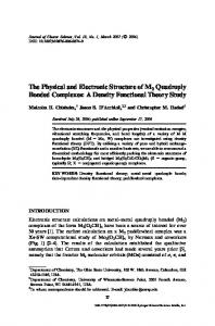
Figure 1. Demixing phase diagram of the AO model for size ratio q = 0.6. The binodal (thick curve), spinodal (dashed curve), tie lines (thin curves), FW line (dotted curve), critical point (dot) and intersection of the binodal and the FW line (cross) are shown for (a) the reservoir representation using the colloid packing fraction ηc and polymer reservoir fraction ηp,r as variables and (b) the system representation using ηc and the actual polymer fraction ηp as variables. The FW line denotes the line where the asymptotic decay of pair correlations crosses over from monotonic to oscillatory. Note that these phase diagrams display only the fluid portion of the phase diagram; a fluid–solid transition occurs for higher values of ηc .

ηp =

12θ13

+

θ14 θ2 /ηc 2 15qθ1 θ2 + 6q 2 θ1 θ22

+ q 3 θ23

,

(73)

where θ1 = 1 − ηc , and θ2 = 1 + 2ηc . Results obtained in one representation are easily converted to the other using equation (72). In figure 1 we display the demixing phase diagram for size ratio q = 0.6. In the reservoir representation (figure 1(a)), we see that the form of the phase diagram does resemble the gas–liquid portion of the phase diagram of a simple substance provided the polymer reservoir density ηp,r is replaced by inverse temperature. Upon increasing ηp,r the system separates into phases with different compositions and the tie lines connecting coexisting phases are horizontal in this representation. The binodal and spinodal coincide at the (lower) critical point. Also shown in figure 1 is the FW line, which divides the phase diagram into regions where the asymptotic decay of pair correlations is either monotonic or oscillatory. We shall discuss this in detail in section 3.5. The actual polymer density in the system may be considerably different from that in the reservoir, because insertion of polymers into the system is hindered by the presence of the colloids, i.e. ηp < ηp,r . The phase diagram in the system representation (figure 1(b)) shows the mixed one-phase region in the lower left part and the demixed two-phase region in the upper right part of the ηc , ηp plane. The tie lines between coexisting phases now have a negative slope. Changing the size ratio q has a pronounced effect on the location of the binodal. We display results for q = 0.4, 0.6, 0.8, 1 in figure 2. As q increases, the binodals move to higher ηp,r , and the critical point shifts to lower colloid fractions ηc (see figure 2(a)). The actual polymer density ηp at the critical point increases slowly with q (figure 2(b)). 3.3. Direct correlation functions We now shift our attention to the structural properties of the bulk AO mixture, focusing first on the pair direct correlation functions ci(2) j (r ). Recall that for binary HS mixtures the


9369

0.3

0.8

DEMIXED

1

1

0.8

0.8

0.6

0.7

DEMIXED

0.6 0.4

lat

or

y

0.2 0.4

cil

0.6

os

ηp

MIXED

ot on

0.5

on

monotonic

m

ηp,r

0.4

0.3

osc

illa

(b)

(a)

MIXED 0

0

ic

0.1

0.1

0.2

ηc

0.3

0.4

0.5

0

0.1

0.2

ηc

0.3

tor

y

0.4

Figure 2. Phase diagram of the AO model for size ratios q = 0.4, 0.6, 0.8, 1. The binodals (thin curves), critical points (dots joined by a thick curve) and intersections of the FW line and the binodals (crosses joined by a dashed curve) are shown for (a) the reservoir representation with ηc and ηp,r and (b) the system representation with ηc and ηp .

ci(2) j (r ) obtained from solving the PY closure are surprisingly simple (polynomial) expressions. Considerable insight into the structure of HS fluids was gained by introducing a new geometrical interpretation of the direct correlation functions [40]. This insight eventually led to the development of the FMT density functional for HS. In the present work the opposite route is followed. Here, starting from the functional we developed in section 2, the ci(2) j (r ) are obtained as second functional derivatives with respect to the density fields. This yields an (approximate) geometrical representation of the pair direct correlation functions of the AO model. Explicit analytic expressions are given below. It is important to note from the outset that the ci(2) j (r ) derived from the present DFT are not (except for special cases) equivalent to those obtained by solving the PY closure for the AO model. In particular, the core condition on the pair correlation functions, gi j (r < Ri + R j ) = 0, is violated in the present approximation, if pair and direct correlation functions are related via the OZ relation. Nevertheless, in the light of the discussion of section 2.6, we do expect ci(2) j to be similar to those from PY. Recall that the latter can only be obtained numerically for the AO model. The direct correlation functions are given by δ 2 β Fexc ij = − ci(2) ( r , r ) = − ψνγ wνi ⊗ wγj , (74) j δρi (r )δρ j (r ) ν,γ

ij where the ⊗ denotes the convolution and ψνγ = ∂ 2 / ∂n iν ∂n iγ , and as usual i, j = c, p. is the free-energy density given by equations (24)–(31). Carrying out this analysis reveals that the bulk direct correlation functions possess the following structure: (2) (2) (ηc , ηp ; r ) = chs (ηc ; r ) + ηp c∗(2) (ηc ; r ), ccc

(75)

(2) (2) ccp (ηc , ηp ; r ) = ccp (ηc ; r ),

(76)

(2) (ηc , ηp ; r ) = 0, cpp

(77)

(2) is the solution of the PY closure for one-component HS. The simple dependence where chs on ηp originates from the linearity of Fexc in the polymer density profile. This dependence (2) (2) allows ccc to be split into two parts: chs is the residual contribution, present even if polymers (2) are absent, while c∗ is the contribution from introducing the polymers, i.e. the function c∗(2)

9370

M Schmidt et al

describes the part of the direct correlations between pairs of colloid due to the presence of (2) the polymers. The spatial dependence of c∗(2) is similar to that of chs , and will be discussed (2) below. Linearity of the functional in ρp (r ) implies that ccp is independent of the polymer (2) density. The size ratio q determines the shape of ccp . Finally, the linearity ensures that the polymer–polymer direct correlation function vanishes, as in the PY closure for the AO model. These observations are, of course, consistent with the low density expansion of ci(2) j used in the alternative derivation of the functional given in section 2.6. i The range of the ci(2) j is determined by the geometric nature of the weight functions wν . As these are characteristic of single-particle geometries, it is clear that the ci(2) j must vanish (2) beyond a separation which is the sum of both particle radii involved, i.e. ci j (r > Ri + R j ) = 0, as is found in the PY treatment. Clearly, this property reflects the approximate nature of the functional. In an exact treatment we would expect contributions beyond the range Ri + R j . We now give explicit expressions for ci(2) j entering equations (75)–(77). Recall that the PY solution [41] for HS with packing fraction ηc and diameter σc (≡ 2Rc ) is (2) chs (ηc ; x) = −

(σc − r ) hs i τ x, (1 − ηc )4 i i

(78)

where τihs are functions of the colloid packing fraction ηc and x = r/σc . The only non-vanishing coefficients are τ0hs = (1 + 2ηc )2 , 3ηc (2 + ηc )2 , τ1hs = − 2 ηc τ3hs = (1 + 2ηc )2 . 2

(79)

(2) is given by The polymer contribution to ccc

c∗(2) (ηc ; r ) = −

(σc − r ) ∗ i τi x , 2q 3 i

(80)

where the only non-vanishing coefficients are τ0∗ = 2[1 + A + 2 Aγ + 4Bγ + 6Bγ 2 + 3Cγ 2 (3 + 4γ )], τ1∗ = −3 − 2 A + (2B)/3 − 6 Aγ − 8Bγ − 18Bγ 2 − 2Cγ [−1 + 9γ (1 + 2γ )], τ3∗ = 1 + 2 Aγ + 6Bγ 2 + 12Cγ 3 ,

(81)

where A, B, C and γ are defined below equation (69). The limiting form at small colloid density is −2(1 + q)3 + 3(1 + q)2 x − x 3 , r < σc , (2) c∗ (ηc → 0; r ) = (82) 0, otherwise. The colloid–polymer direct correlation function is given by  2 3 −(1 + γ )(1 r < |Rc − Rp |   + Aγ + 2Bγ + 3Cγ ),  i (2) τcp,i x , |Rc − Rp | r |Rc + Rp | (ηc , r ) = −(1 + γ ) ccp  i   0, otherwise,

(83)


9371

where the only non-vanishing coefficients are 3γ τcp,−1 = − (1 − q)2 [3 + q + 3γ (1 + q)]2 , 32 τcp,0 = 12 {2 + γ [7 + 3γ (5 + 3γ ) + 9γ q 2 + (1 + 3γ )2 q 3 + 3q(1 + q)]}, (84) 3γ τcp,1 = − [5 + 3γ (4 + 3γ ) + 2q + 6γ q + (q + 3γ q)2 ], 4 γ τcp,3 = (1 + 3γ )2 . 2 In the limit ηc → 0 the colloid–polymer direct correlation function reduces to the colloid– polymer Mayer function f cp (r ), i.e. −1, r < Rc + Rp (2) ccp (ηc → 0; r ) = (85) 0, otherwise. Simpler expressions are obtained in the special case q = 1, where only a single length scale (2) (2) (2) (ηc ; r ) and ccp = chs (ηc ; r ). It follows that is present, and one can use c∗(2) = ∂η∂ c chs (σc − r ) τ ∗x i , (86) c∗(2) (ηc ; r ) = − (1 − ηc )5 i i where the only non-vanishing coefficients are τ0∗ = 4(2 + ηc )(1 + 2ηc ), τ1∗ = − 23 (2 + ηc )[2 + ηc (9 + ηc )], τ3∗ = 12 (1 + 2ηc )[1 + ηc (9 + 2ηc )].

(87)

In order to illustrate the variation with r and ηc , we plot the various functions, for q = 0.6, (2) (r ) is shown in figure 3(a) with ηc in the range 0–0.4. This is the contribution to in figure 3. chs (2) ccc arising solely from the ‘bare’ colloids. The polymers generate an (additive) contribution (2) (r ). ηp c∗(2) (r ), where the function c∗(2) (r ), plotted in figure 3(b), has a similar form to chs Changing the size ratio q does not dramatically alter the shape; it merely changes the vertical (2) (r ) for the same values of ηc . This function is scale of the plot. Finally, figure 3(c) shows ccp constant for r < |Rc − Rp | = 0.2σc and vanishes for r > |Rc + Rp | = 0.8σc , for the present size ratio. All three functions become more negative in the core region as ηc is increased. Note (2) through the linear dependence in equation (75). that the polymer density ηp only enters ccc Summarizing, we find it remarkable that the direct correlation functions for the AO model, which is characterized by two thermodynamic variables ηc and ηp , can be described by relatively simple analytic expressions and that all relevant information, for a given size ratio q, can be condensed into as few as three plots. 3.4. Structure factors and criticality The total pair correlation functions h i j (r ) = gi j (r ) − 1, where gi j (r ) are pair correlation functions, are related to the direct correlation functions ci(2) j (r ) via the mixture OZ relations [41]. These simplify in Fourier space: h cc (k) =

(2) (2) (2) (2) ccc (k) + ρp [(ccp (k))2 − ccc (k)cpp (k)] D(k)

(88)

h pp (k) =

(2) (2) (2) (2) cpp (k) + ρc [(ccp (k))2 − ccc (k)cpp (k)] D(k)

(89)

h cp (k) =

(2) ccp (k) , D(k)

(90)

9372

M Schmidt et al 0

0

−5

− 100

c*(2)(r)

chs(2)(r)

− 10

− 15

− 200

− 300

− 20

(a) − 25

0

0.5

(b) − 400

1

0

0.5

r/σc

1

r/σc 0

Rc− Rp

−2

(2)

ccp (r)

−4

−6

Rc+Rp

−8

(c) − 10

0

0.5

1

r/σc Figure 3. Pair direct correlation functions for ηc = 0, 0.1, 0.2, 0.3, 0.4 (from top to bottom) (2) (2) (r) to ccc (r); obtained for the AO model with size ratio q = 0.6: (a) colloid contribution chs (2) (b) polymer contribution c∗(2) (r) to ccc (r); (c) full colloid–polymer direct correlation function (2) (r). These results are obtained from equations (78), (80), (83). ccp

where h i j (k) is the three-dimensional Fourier transform of h i j (r ) and the common denominator is given by (2) (2) (2) (k)][1 − ρp cpp (k)] − ρc ρp [ccp (k)]2 . D(k) = [1 − ρc ccc

(91)

The corresponding partial structure factors Si j (k) then can be obtained via [41] Si j (k) = δi j + (ρi ρ j )1/2 h i j (k).

(92)

It is sometimes useful to describe the like–like structure factors by means of the OZ relation Sii (k) = 1/(1 − ρi cii(2),eff (k)),

(93)

that has the same formal structure as the OZ relation for a one-component system, and that employs an effective direct correlation function given by cii(2),eff (k) = cii(2) (k) +

2 ρ j ci(2) j (k)

1 − ρ j c(2) j j (k)

.

(94)

It is straightforward to show that equations (93) and (94) are completely equivalent to the standard mixture formulation of equations (88)–(92). So far all is general but now we note


9373

(2) that in the present approximation cpp = 0, see equation (77). This leads to rather simple expressions for the effective direct correlation functions: (2),eff (2) (2) (k) = ccc (k) + ρp ccp (k)2 , ccc (2),eff cpp (k) =

1

(2) ρc ccp (k)2 . (2) − ρc ccc (k))

(95) (96)

In particular, equation (96) with (93) allows us to understand why Spp can be significantly (2) different from unity, the ideal gas result, even though cpp = 0. Results for Si j (k) and gi j (r ) were presented in an earlier letter [31]. We found that for q = 0.15, ηc = 0.3 and ηp = 0.05 all three partial pair correlation functions were close to the corresponding PY results. The latter were obtained numerically [8]. For q = 0.1, ηc = 0.25, ηp = 0.107 we compared our results for Scc (k) and gcc (r ) with those of simulation (for this small size ratio there is an exact mapping to an effective one-component colloid system for which simulations are easily performed [5]). The overall agreement was reasonable, although the structure factor was a little out of phase and the results of the DFT strongly underestimated the very high contact value gcc (σc ) and violated (weakly) the core condition gcc (r ) = 0, r < σc . In the present study, we are concerned with less extreme size ratios where the effective (depletion) potential between colloids is longer ranged and less deep near contact than the cases investigated earlier and we expect the DFT to fare somewhat better. An important advantage of the present DFT approach (over most integral equation theories) is that the thermodynamic and structural routes to the spinodal, binodal and, therefore, the critical point are consistent. In particular, the spinodal line, equation (73), can equally well be found by considering the locus of divergence of Si j (k), i.e. the vanishing of D(k) in equation (91). This consistency is especially important in the vicinity of the critical point. The location of the critical point in the ηc , ηp,r plane can be obtained by tracing the coexistence densities towards small ηp,r , but careful numerical work is needed to obtain accurate results. In the present case, the critical point can be obtained in a simpler way: starting from the spinodal in the system representation, equation (73), we switch to the reservoir representation using equations (72), (69), and obtain the spinodal polymer reservoir density spin as a function of colloid density, ηp,r (ηc ). As the critical point is at the minimum of this function, finding the minimum is a stable and numerically trivial operation. For states slightly removed from criticality we expect OZ behaviour: Si j (k) = Si j (0)/[1 + ξ 2 k 2 + O(k 4 )], where the correlation length ξ is the same for all pairs i j . This general result is a direct consequence of the OZ relations for a mixture (88)–(90) and follows from the fact that D(k) is the common denominator for all pairs, equation (91). As the Si j (k) are given analytically in the present theory, we can confirm explicitly the OZ behaviour. We find that the common correlation length diverges with the mean-field exponent ν = 1/2 and on a path at fixed ηc = ηccrit we define the amplitude ξ0 via ξ = ξ0 /(ηpcrit − ηp )1/2 . ξ0 /σc depends only on the size ratio q. It is roughly proportional to the mean of the colloid and polymer diameters and is conveniently expressed as √ ξ0 = 12 (σc + σp )/K (q), where typical values are K (q) = 3.00, 2.36, 5, for q = 0.4, 0.8, ∞, respectively. Note that σp = 2Rp . Figure 4 displays the partial structure factors calculated for q = 0.6 and a fixed value of ηc , equal to the critical point value ηccrit = 0.1843. Results are presented for four values of ηp,r , corresponding to the critical ‘isochore’ in figure 1(a). For ηp,r = 0 (no polymer) Scc (k) is simply the (PY) HS structure factor for ηc = 0.1843. Upon increasing ηp,r , Scc (k) develops a maximum at k = 0, OZ behaviour ensues and then, at the crit = 0.4943, Scc (0) → +∞. Spp (k) has a somewhat different variation. This critical value ηp,r function develops its leading maximum at k = 0 for very small polymer fractions and Spp (0) crit is very large even for ηp,r = 0.36, well away from the critical point. As ηp,r → ηp,r , Spp (0)

9374

M Schmidt et al 3

Scc Scp Spp

Sij(k)

2

1

0

-1 0

5

10

15

20

k σc Figure 4. Partial structure factors Scc , Scp , Spp for size ratio q = 0.6 at fixed colloid fraction ηc = ηccrit = 0.1843, and increasing (indicated by arrows) polymer reservoir density ηp,r = crit = 0.4943. On approaching the critical point, along a vertical path in the phase 0, 0.2, 0.36, ηp,r diagram of figure 1(a), Scc (k) and Spp (k) become increasingly positive and Scp (k) increasingly negative at small wavenumbers k. Note that for ηp,r = 0, Scc (k) corresponds to the pure HS structure factor.

diverges in the same fashion as Scc (0). By contrast, Scp (0) becomes increasingly negative and diverges to −∞ on approaching the critical point. Similar features are found for other size ratios. The form of Spp (k) is particularly striking and has repercussions for the distribution of polymer in the mixture. Note that similar shapes of Spp (k) were found in PY calculations [7, 8] for the AO mixture. 3.5. Asymptotic decay of correlations: Fisher–Widom line The pair correlation functions gi j (r ) should exhibit qualitatively different asymptotic decay at different points in the phase diagram. In the neighbourhood of the critical point gi j (r ) will decay monotonically, as befits OZ behaviour, whereas for small values of ηp,r the mixture is HS-like and the gi j (r ) should exhibit damped oscillatory decay as r → ∞. Thus upon varying the thermodynamic parameters ηp,r and ηc the ultimate decay of gi j (r ) should change from being oscillatory to purely monotonic [42–45]. The line in the phase diagram separating the two types of decay is termed the FW line [42] after the authors who introduced the concept. This is not a line of thermodynamic singularity. Rather it indicates crossover to different structural regimes. Although the FW line is defined by considering the decay of bulk pair correlation functions, it plays a key role in inhomogeneous situations since the asymptotic decay into bulk of one-body density profiles is determined by the same physical considerations. Thus it is relevant for several interfacial phenomena [32, 43, 44, 46]. In order to calculate the FW line, we again exploit the fact that our partial structure factors are given analytically. Since the asymptotic decay of gi j (r ) is determined by the singularities of the Si j (k) in the complex plane our strategy is to trace the locations of these. We denote these singularities k = a1 + ia0 . Oscillatory behaviour, h i j (r → ∞) ∝ cos(a1r ) exp(−a0r )/r , stems from poles with non-zero real part a1 , whereas monotonic behaviour, h(r → ∞) ∝ exp(−a0r )/r , stems from poles residing on the imaginary axis, a1 = 0. The ultimate decay is governed by the pole with the smallest imaginary part a0 [44]. We obtain the location of the singularities by finding the roots of 1/|Si j (k)| = 0 numerically, taking appropriate starting values. This is equivalent to finding the zeros of D(k), equation (91), in the complex plane.


9375

1.4

DEMIXED

2

1.2 1.5 0.4

MIXED ηp/ηpcrit

crit ηp,r /ηp,r

0.8

0.6 0.6

0.8

0.4

0.6 1 0.8

DEMIXED

1 0.5

(a)

ic oton mon illatory osc

0.2 0

(b)

0.4

1

0.5

monotonic oscillatory

MIXED 0

0

1

1

crit

ηc /η c

1.5

2

0

0.5

1

ηc /ηcrit c

1.5

2

Figure 5. FW lines for size ratios q = 0.4, 0.6, 0.8, 1 plotted in scaled variables. The FW lines are denoted by solid curves; the dotted extensions are metastable, i.e. they lie inside the binodal. The intersections of the FW lines and the binodal are crosses joined by a dashed curve. (a) Scaled crit ; (b) scaled system representation with η /ηcrit reservoir representation with ηc /ηccrit and ηp,r /ηp,r c c crit and ηp /ηp . For each q, increasing ηp,r or ηp at fixed ηc leads to crossover from monotonic to oscillatory decay at the FW line.

Note that all partial structure factors possess the same singularities, because of the common denominator D(k). That is why all the h i j (r ) exhibit the same exponential decay length a0−1 and, when oscillatory, the same wavelength 2π/a1 , and why there is a single FW line that characterizes the crossover in a mixture. In practice we chose Scc (k) and calculated the pole with the smallest a0 residing on the imaginary axis and also the pole with the smallest a0 but with a1 > 0. At fixed ηc , we varied ηp until the imaginary parts a0 of both poles were identical, giving a point on the FW line. Following this procedure for all ηc maps out the complete FW line for a given size ratio. In figure 1 we plot the FW line for q = 0.6 in both the reservoir and system representations. The FW line intersects the binodal on the colloid-rich side (liquid) and is bounded at high ηp,r by the liquid spinodal. For this size ratio the overall shape and location of the FW line appears similar to that found [43, 45] for simple fluids, whose interatomic pair potential is of finite range and which exhibit liquid–gas phase separation, once we recall that ηp,r is equivalent to inverse temperature. Figure 2 displays the intersection of the FW line with the binodal for several values of size ratio q. As q increases the intersection occurs further from the critical point, exposing a larger range of monotonic decay along the liquid side of the crit binodal. In figure 5 we plot the FW lines in terms of the scaled variables ηc /ηccrit and ηp,r /ηp,r (or ηp /ηpcrit ) for four values of q. As q increases we observe that a larger portion of the scaled phase diagram lies on the monotonic side of the FW line. For q = 0.4 the FW line lies just below the critical point and most of the single-phase portion of the scaled phase diagram now falls on the oscillatory side. This might reflect the fact that for q = 0.4 (and smaller values of q) the FW line exhibits a minimum when plotted in the reservoir representation, figure 5(a). The presence of the minimum implies that on increasing ηc at an appropriate fixed ηp,r the decay of correlation functions should change from monotonic to oscillatory to monotonic and, finally, to oscillatory. Whether such behaviour reflects the fact that the fluid–fluid phase separation should be close to becoming metastable (w.r.t. fluid–solid) for these small values of q can only be ascertained by more sophisticated treatments. What is probably more relevant for a real colloid–polymer mixture is figure 5(b) which shows that in the system representation there is a maximum in the FW line for all four values of q. Thus increasing ηc at a sufficiently

9376

M Schmidt et al

3

3

Im(kσc)

4

Im(kσc)

4

2

1

2

1

(a) 0 0

2

4

6

(b) 0 0

8 10 12 14

Re(kσc)

4

4

6

8 10 12 14

Re(kσc)

4

Im(kσc)

3

Im(kσc)

3 2

1 0 0

2

2

1

(c) 2

4

6

8 10 12 14

Re(kσc)

0 0

(d) 2

4

6

8 10 12 14

Re(kσc)

Figure 6. Absolute value of the colloid–colloid structure factor |Scc | in the complex plane for size ratio q = 0.6 at fixed colloid fraction ηc = ηccrit = 0.1843, and four values of polymer reservoir density ηp,r : (a) pure HS, ηp,r = 0 (ηp = 0); (b) ηp,r = 0.2 (ηp = 0.07161) in the oscillatory regime; (c) on the FW line, ηp,r = 0.36 (ηp = 0.1290); (d) at the critical point, ηp,r = 0.4943 (ηp = 0.1770). Arrows indicate the (smallest) purely imaginary pole. This pole lies at the origin in (d). Bright (dark) colour indicates large (small) values. Note that these statepoints are the same as in figure 4.

small fixed polymer fraction ηp should lead to crossover from monotonic to oscillatory back to monotonic decay of correlations (see also figure 1(b)). Finally, we remark that in the limit ηp,r → 0, the FW line smoothly approaches the origin, ηc = 0. This is to be expected, since for pure HS g(r ) exhibits oscillatory decay for all non-zero values of the packing fraction. Such behaviour is equivalent to that found for simple fluids in the limit T → ∞ [45]. We can summarize and visualize much of what is described in this subsection by analysing the behaviour of the structure factors in the complex plane, and in figure 6 we report results for |Scc (k)| with q = 0.6, taken along the same critical ‘isochore’, ηc = ηccrit , as in figure 4. Pure HS (figure 6(a)) do not possess a pole on the imaginary axis so the two maxima correspond to complex poles; the dominant one corresponds to a1 σc ∼ 2π. Upon increasing the polymer reservoir density to ηp,r = 0.2 (figure 6(b)), a pole appears on the imaginary axis and this moves downwards with ηp,r , until its value equals that of the imaginary part of the neighbouring complex pole (figure 6(c)) defining a point on the FW line. At the critical point, the pole on the imaginary axis reaches the origin (figure 6(d)). This pole leads to the divergence of the physical structure factors, Si j (k → 0), at the critical point. Figure 4 displays the physical structure factors at the same statepoints. 3.6. Effective interaction between colloids: depletion potential In their original study Asakura and Oosawa [1] determined the effective potential, VAO (r ; z p ), between two HS colloids (or macroparticles) in a sea of ideal polymer of fugacity z p . Their celebrated potential is attractive in the range 2Rc < r < 2(Rc + Rp ) and vanishes for larger


9377

separations r . The attraction arises from the depletion effect whereby polymer is excluded or depleted from the region between the colloids when the separation of their surfaces is 2Rc , which implies the PY results for the contact value gcc (2Rc+ ) are too small [8, 47, 48]. Given that our present DFT bears a close resemblance to the PY approximation we might expect to observe similar failings [31]. The advantage here is that we have explicit, analytic results for ci(2) j so it is straightforward to analyse the behaviour of correlations in the low ηc limit. From equations (75), (78), (80), (82) we can ascertain (2),eff (r ) given by the Fourier transform of equation (95). Since the limiting behaviour of ccc (2) (2) ccc (ηp ; r ) = 0 for r > 2Rc and ccp (ηc → 0; r ) = f cp (r ) it follows that DFT predicts, for ηc → 0, (2),eff ccc (r ) = −βVAO (r ; z p ),

r > 2Rc ,

(100)

where we used the fact that z p = ρp,r = ρp in the limit ηc → 0. Thus our DFT does not yield the exact limiting result (99); the latter only reduces to (100) in the limit z p → 0. The present approach, via the OZ route to the pair correlation functions, suffers from the same failing as the PY approximation. Clearly both approximation schemes fail to incorporate the physical ingredients which are required to exponentiate −βVAO . However, we must not infer that the present DFT fails to incorporate the depletion effect which is, after all, the crucial feature of colloid–polymer mixtures. We have already seen in section 3.1 that the bulk free energy of the mixture acquires an attractive contribution; this contribution can only arise from the depletion effect. Moreover, the theory does generate an (2),eff , equation (100), albeit one that is too weak. attractive contribution in ccc Within DFT the OZ route is not the only one to pair correlation functions. The alternative is the test particle route, whereby one fixes a particle of species i at the origin and determines the inhomogeneous one-body density profile ρ j (r ) arising from the external potential Vi j (r ) exerted by the fixed particle. It follows that gi j (r ) = ρ j (r )/ρ j (∞). In applying the test particle prescription one solves the Euler–Lagrange equations for the one-body densities so all

9378

M Schmidt et al

that is required are the one-body direct correlation functions ci(1) (r ); these involve only a first derivative of Fexc , see equation (60). One can show that in the limit ηc → 0, the test particle route for the present DFT yields the exact result gcc (r ) ≈ exp(−βVAO (r ; z p )). An instructive way of obtaining this result is to implement the procedure developed by Roth et al [38] for calculating the depletion potential. The latter is given by −βVdep (r ; z p ) = lim [cc(1) (r ) − cc(1) (∞)], z c →0

(101)

where cc(1) (r ) refers to the situation where a colloid, fixed at the origin, exerts its field on the polymer and on a (test) colloid inserted at r [38]. cc(1) (r ) is easily calculated for the present DFT (the calculation mimics that for the binary HS functional given in [38]) and in the limit where the colloid density vanishes we find that βVdep is proportional to the convolution of two Mayer functions, i.e. it reduces precisely to the second term in equation (98). That the analysis can be performed analytically and the result is much simpler than that for HS mixtures simply reflects the fact that f pp (r ) = 0 in the AO model. With hindsight it is, perhaps, not too surprising that geometrically based DFT should describe correctly the depletion potential; the latter is merely a manifestation of excluded volume effects. Nevertheless, this excercise does indicate that the test particle route to gcc (r ) is likely to be much more accurate than the OZ route, especially for situations where ηc is low and ηp,r is high so that the depletion potential is strongly attractive and contact values gcc (2Rc+ ) are very large. The test particle route also has the advantage that it guarantees that gcc (r ) = 0 for r < 2Rc and gcp (r ) = 0 for r < Rc + Rp . 4. Discussion We have derived a DFT for the binary AO mixture based on geometrical information about the hard and ideal spheres which constitute the AO model. Our FMT approach follows the strategy which was employed successfully for other model systems. Imposing the correct dimensional crossover on the functional, section 2, appears to provide a systematic procedure for deriving approximate DFTs. Whether the procedure can be implemented explicitly depends on the particular model. In the present case, as for penetrable spheres [25], the Widom– Rowlinson model [26], a needle–sphere model [28], a model amphiphilic mixture [29] and a ternary mixture of colloids, polymers and needles [30], the procedure is tractable and leads to a relatively simple functional. An alternative derivation, section 2.6, which corresponds to linearizing the Rosenfeld functional for a binary HS system w.r.t. the density of one of the species, yielded the identical functional. Multi-component mixtures can also be treated by our procedures. For example, if a three-component mixture of HS of two different sizes plus polymer were required one would take the Rosenfeld HS functional for a ternary mixture of HS and linearize in one of the densities which is then identified as (ideal) polymer. Similarly, if a three-component mixture of HS plus two polymer species were required one would simply linearize the ternary HS functional w.r.t. two densities. The corresponding functionals are again identical to those obtained from application of the recipe outlined in section 2.4, where the generating zero-dimensional free energy F0d is replaced by that for the corresponding ternary mixture. In fact the free energy for the ternary system is simply equation (14) with colloid (polymer) packing fraction replaced by the sum of packing fractions of colloid (polymer) species. In section 2.7 we described the concept of integrating out degrees of freedom within the context of DFT. The present functional affords a valuable example because the Euler– Lagrange equations decouple in this case and cp(1) (r ) is a functional of the colloid profile alone. It is important to emphasize, however, that the mapping to an effective one-component


9379

fluid of colloids that is implicit within the approximate DFT treatment is not equivalent to that which is obtained by an explicit and exact integrating out of polymer coordinates in the partition function. Recall that this latter route yields an effective Hamiltonian containing only one- and two-body contributions when q < 0.1547. This particular size ratio has no special significance within our approximate DFT. Our present paper focuses on the properties of bulk fluid phases. We found that the bulk free energy of the AO mixture is identical to that derived from the free-volume theory of Lekkerkerker et al [4] and we pointed out some of the connections between the two approaches (see section 3.1), emphasizing that both impose linearity of the free energy in the polymer density. Since the two theories yield the same free energy, they predict identical fluid–fluid phase separation, i.e. the same binodal and spinodal. The latter can be determined analytically from equation (73), which is particularly useful for critical point studies. How accurate is the free-volume theory for the phase separation curve? When we completed our paper there were no systematic studies of the full binary AO model for the range of size ratios q where fluid– fluid phase separation occurs. Published studies consider either the effective one-component Hamiltonian (97) keeping only pair potential [5], which is strictly valid for q < 0.1547, or a lattice polymer version [6]. It is well known that treating highly asymmetric mixtures by brute force simulation is beset by ergodicity problems and slow equilibration when the packing fraction of the smaller species is large. A new study by Dijkstra [47] indicates that for q = 1 the fluid–fluid binodal does lie rather close to the free-volume result. This also seems to be the case for other values of q [50] and the current indications are that free-volume theory (and, therefore, our present DFT) does provide a reasonable account of the location of the fluid–fluid binodal in the ηc , ηp,r plane for those values of q(> 0.35) where fluid–fluid phase separation is stable w.r.t. fluid–solid. We have not considered solid phases in the present study. These could be investigated within the framework of the present DFT which would enable us to calculate the full phase diagram. Existing studies [4, 5] based on free-volume ideas employ the expression of Hall [49] for the Helmholtz free-energy density of the HS solid entering equation (71) and the same expression for the free-volume fraction α(ρc ) as used for fluid phases. It would be interesting to compare DFT predictions for the (rich) fluid–solid phase equilibria in this model with those from other approximate theories and with simulation. Note i (r ), entering 3 in that the tensor contribution, which depends on the weight function wˆ m2 equation (31) is crucially important for the inhomogeneous solid phase [21, 22] but makes no contribution to the free energy of a homogeneous fluid phase. An important feature of our present DFT is that pair correlation functions of the bulk fluid can be obtained very easily via the OZ route (sections 3.3 and 3.4). Thus the theory is much easier to implement than the PY integral equation theory for the AO mixture which can only be solved numerically [7, 8]. The pair direct correlation functions and the partial structure factors Si j (k) are given analytically, as is the case in the PY approximation for HS mixtures. What is remarkable here is that the AO mixture exhibits pure entropically driven fluid–fluid phase separation so that the Si j (k) display a divergence at a spinodal line which is identical to that obtained from the bulk free energy. This type of consistency is, of course, a direct consequence of the DFT approach. Having analytical results for the Si j (k) also enabled us to obtain directly the FW line (section 3.5), describing the line of crossover from monotonic to oscillatory asymptotic decay of the total pair correlation functions h i j (r ). To the best of our knowledge this is the first time the FW line has been investigated in detail for this type of system. One intriguing feature, which warrants further attention, is the nature and location of the FW line as q becomes smaller and the fluid–fluid critical point shifts to lower ηp and higher ηc (figure 2). For q = 0.4 the monotonic regime, where h i j (r ) exhibit OZ-like decay at large r , is restricted to a narrow portion of the phase diagram near the critical point—see

9380

M Schmidt et al

figure 5. This might be a structural indicator that the fluid–fluid phase separation is becoming metastable w.r.t. fluid–solid. We expect the accuracy of the h i j (r ) and Si j (k) obtained from the OZ route to be comparable with that of the PY approximation for the AO mixture. As remarked in section 3.6, both approximations fail to reproduce the correct limiting behaviour of gcc (r ) as ηc → 0. This is particularly significant for small size ratios at states with low ηc and high values of ηp,r where the depletion potential is very deep and very short ranged. Neither PY nor the present theory can be expected to yield accurate pair correlation functions in this regime. The DFT has the additional drawback of not enforcing the core conditions gcc (r < 2Rc ) = 0 and gcp (r < Rc + Rp ) = 0. These core conditions constitute implicit (hidden) constraints when viewed from the perspective of taking functional derivatives to obtain ci(2) j (r ) and then inverting to obtain gi j (r ). In principle, one might exploit the core conditions in order to derive (more sophisticated) approximations for the free-energy functional. In practice, such a procedure would be extremely difficult to implement. (In this context it appears remarkable that Rosenfeld’s HS functional does yield gi j (r ) that fulfill the core conditions. Of course, it is by virtue of the fact that the ci(2) j generated from the Rosenfeld functional are those of PY that the resulting gi j (r ) do satisfy the core condition.) DFT provides an alternative route to gi j (r ), namely the test-particle procedure, and we have argued that this is likely to yield significantly better results than the OZ route, especially for situations where the depletion attraction is very strong. Once again systematic comparisons with simulation results are required in order to assess further the degree of consistency and, therefore, the reliability of the DFT. Note that the OZ and test particle routes do yield identical results for the decay length a0−1 and wavelength 2π/a1 , characterizing the asymptotic decay of the pair correlation functions. It follows that the FW lines calculated from both routes are identical. The experience gleaned from the present study of bulk properties gives us confidence in applying our DFT to inhomogeneous fluids where the spatial variation of the density profiles arises from the imposition of external fields. Since the DFT incorporates fluid–fluid phase separation it has been applied [9, 32] to

(i) the planar interface between coexisting colloid-rich and colloid-poor phases—the density profiles of both colloid and polymer exhibit oscillations on the colloid-rich (liquid) side of the interface provided the bulk liquid lies on the oscillatory side of the FW line—and (ii) the study of wetting phenomena for the mixture adsorbed at a hard wall. The interface between the wall and the colloid-poor phase is partially wetted by the colloid-rich phase crit ). at high ηp,r but is completely wet at low ηp,r (> ηp,r A novel sequence of layering transitions accompanies the transition to complete wetting. It was argued [32] that the surface phase behaviour reflects the presence of many-body contributions to the effective one-component Hamiltonian for the colloids. Such contributions are included implicitly in the DFT. Other adsorption problems which can be tackled by our DFT include possible wall-induced crystallization (depletion at a hard wall leads to a very high contact density for colloids [13]) and wetting of the wall–fluid interface by the crystalline phase. Mixtures confined by planar walls or in other geometries are readily tackled which means that phenomena such as capillary condensation can be investigated in detail. Sedimentation in a gravitational field, behaviour in laser fields and the properties of solid–fluid interfaces are also topics ripe for investigation.


9381

Acknowledgments We thank M Dijkstra, R van Roij, R Roth, A Lang, P Tarazona, M Fuchs and I Götze for many helpful discussions. This research was supported by the British–German ARC Programme (project104b). Appendix A. Weight functions in Fourier space For completeness we list the (three-dimensional) Fourier transforms of the first six weight functions listed in equations (17)–(22): 4π [k Ri cos(k Ri ) − sin(k Ri )], k3 4π Ri sin(k Ri ), w2i (k) = k sin(k Ri ) , w1i (k) = k sin(k Ri ) , w0i (k) = Ri k k 4π i wv2 (k) = 2 [k Ri cos(k Ri ) − sin(k Ri )] , k k k Ri cos(k Ri ) − sin(k Ri ) k i , wv1 (k) = k 2 Ri k

w3i (k) = −

(A.1) (A.2) (A.3) (A.4) (A.5) (A.6)

where k = |k|. Appendix B. Density functional in two dimensions In the following we present the DF for the two-dimensional AO model obtained from the route described in section 2.6 starting from the two-dimensional Rosenfeld hard disc functional (see e.g. [20]). The excess free energy Fexc has the general structure, equation (15) of a two-dimensional integral over a free-energy density. The weighted densities are obtained by two-dimensional convolutions (B.1) n iν (x) = d 2r ρi (r )wνi (x − r ), of the four two-dimensional weight functions wdi (r ) = (Ri − r ),

(B.2)

w1i (r ) = δ(Ri − r ), i wv1 (r ) = δ(Ri − r )r /r, i w0 (r ) = δ(Ri − r )/(2πr ),

(B.3) (B.4) (B.5)

where r in equations (B.2)–(B.5) denotes the two-dimensional position vector. The free-energy density is p p n c0 n d n c1 n c1 − ncv1 · ncv1 nd 1 p c c = −(n 0 + n 0 ) ln(1 − n d ) + + + 1 − n cd 4π 1 − n cd (1 − n cd )2 p

+

p

n 1 n c1 − nv1 · ncv1 . 2π(1 − n cd )

(B.6)

9382

M Schmidt et al

References [1] [2] [3] [4] [5] [6] [7] [8] [9] [10] [11] [12] [13] [14] [15] [16] [17] [18] [19] [20] [21] [22] [23] [24] [25] [26] [27] [28] [29] [30] [31] [32] [33] [34] [35]

[36] [37]

[38] [39] [40] [41] [42] [43] [44] [45] [46] [47] [48] [49] [50]

Asakura S and Oosawa F 1954 J. Chem. Phys. 22 1255 Vrij A 1976 Pure Appl. Chem. 48 471 Gast A P, Hall C K and Russell W B 1983 J. Colloid Interface Sci. 96 251 Lekkerkerker H N W, Poon W C K, Pusey P N, Stroobants A and Warren P B 1992 Europhys. Lett. 20 559 Dijkstra M, Brader J M and Evans R 1999 J. Phys.: Condens. Matter 11 10 079 Meijer E J and Frenkel D 1994 J. Chem. Phys. 100 6873 Louis A A, Finken R and Hansen J 1999 Europhys. Lett. 46 741 Dijkstra M, van Roij R and Evans R 2000 J. Chem. Phys. 113 4799 Brader J M 2001 PhD Thesis University of Bristol Leal Calderon F, Bibette J and Biasis J 1993 Europhys. Lett. 23 653 Ilett S M, Orrock A, Poon W C K and Pusey P N 1995 Phys. Rev. E 51 1344 Brader J M and Evans R 2000 Europhys. Lett. 49 678 Brader J M, Dijkstra M and Evans R 2001 Phys. Rev. E 63 041405 de Hoog E H A and Lekkerkerker H N W 1999 J. Phys. Chem. B 103 5274 de Hoog E H A, Lekkerkerker H N W, Schulz J and Findenegg G H 1999 J. Phys. Chem. B 103 10 657 Evans R 1979 Adv. Phys. 28 143 Evans R 1992 Fundamentals of Inhomogeneous Fluids ed D Henderson (New York: Dekker) p 85 Rosenfeld Y 1989 Phys. Rev. Lett. 63 980 Rosenfeld Y, Schmidt M, Löwen H and Tarazona P 1996 J. Phys.: Condens. Matter 8 L577 Rosenfeld Y, Schmidt M, Löwen H and Tarazona P 1997 Phys. Rev. E 55 4245 Tarazona P and Rosenfeld Y 1997 Phys. Rev. E 55 R4873 Tarazona P 2000 Phys. Rev. Lett. 84 694 Cuesta J A 1996 Phys. Rev. Lett. 76 3742 Cuesta J A and Martinez-Raton Y 1997 Phys. Rev. Lett. 78 3681 Schmidt M 1999 J. Phys.: Condens. Matter 11 10 163 Schmidt M 2001 Phys. Rev. E 63 010101(R) Bolhuis P and Frenkel D 1994 J. Chem. Phys. 101 9869 Schmidt M 2001 Phys. Rev. E 63 050201(R) Schmidt M and von Ferber C 2001 Phys. Rev. E 64 051115 Schmidt M and Denton A R 2002 Phys. Rev. E 65 021508 Schmidt M, Löwen H, Brader J M and Evans R 2000 Phys. Rev. Lett. 85 1934 Brader J M, Evans R, Schmidt M and Löwen H 2002 J. Phys.: Condens. Matter 14 L1 Groh B and Mulder B 2000 Phys. Rev. E 61 3811 Percus J K 1976 J. Stat. Phys 15 505 Cuesta J A, Martinez-Raton Y and Tarzona P J. Phys.: Condens. Matter (special issue on density functional theory) Cuesta J A, Martinez-Raton Y and Tarzona P 2002 Preprint cond-mat/0205256 Brader J M and Evans R 2002 Physica A 306 287 A closely related, general scheme for constructing a free-energy functional for the effective one-component fluid and the corresponding hierarchy of effective direct correlation functions is given by Cuesta J A and Martinez-Raton Y 1999 J. Phys.: Condens. Matter 11 10 107 Roth R, Evans R and Dietrich S 2000 Phys. Rev. E 62 5360 Roth R, Evans R and Louis A A 2001 Phys. Rev. E 64 051202 Rosenfeld Y 1988 J. Chem. Phys. 89 4272 Hansen J P and McDonald I R 1986 Theory of Simple Liquids 2nd edn (London: Academic) Fisher M E and Widom B 1969 J. Chem. Phys. 50 3756 Evans R, Henderson J R, Hoyle D C, Parry A O and Sabeur Z A 1993 Mol. Phys. 80 755 Evans R, Leote de Carvalho R J F, Henderson J R and Hoyle D C 1994 J. Chem. Phys. 100 591 Dijkstra M and Evans R 2000 J. Chem. Phys. 112 1449 Archer A J and Evans R 2001 Phys. Rev. E 64 041501 Dijkstra M, private communication Dijkstra M and van Roij R 2002 Preprint Louis A A 2001 Phil. Trans. R. Soc. A 359 939 see appendix A Hall K R 1972 J. Chem. Phys. 57 2252 Bolhuis P G, Louis A A and Hansen J-P 2002 Preprint and cond-mat/020606

Density functional theory for a model colloid–polymer mixture: bulk

Density functional theory for a model colloid–polymer mixture: bulk

Suggest Documents

A density-functional theory for bulk and inhomogeneous Lennard ...

Density Functional for a Model Colloid-Polymer Mixture - Theoretische

A Pooled Subspace Mixture Density Model for

A Density Functional Theory Study

Density Functional Theory for Experimentalists: A

Periodic density functional theory calculations of bulk and the (010 ...

A Comparative Density Functional Theory and Density Functional

Challenging Density Functional Theory

Relativistic density functional theory

Density Functional Theory

Partition Density Functional Theory

Density Functional Theory Calculations

Density Functional Theory

Density Functional Theory

Density functional theory (DFT)

density functional theory study

Machine learning density functional theory for the Hubbard model

Density Functional Theory for Plasmon-Assisted Superconductivity

Density Functional Theory Calculations For MethylBenzene Molecules ...

Density functional theory methods for characterization ...

Time-dependent density-functional theory for ...

Troubleshooting Time-Dependent Density-Functional Theory for

Troubleshooting Time-Dependent Density-Functional Theory for

Koopmans' condition for density-functional theory