Published July, 2000
VANDERBORGHT ET AL.: DERIVING TRANSPORT PARAMETERS FROM TRANSIENT FLOW LEACHING
model to evaluate the performance of wick samplers in soils. Soil Sci. Soc. Am. J. 59:88–92. Risler, P.D., J.M. Wraith, and H.M. Gaber. 1996. Solute transport under transient flow conditions estimated using time domain reflectometry. Soil Sci. Soc. Am. J. 60:1297–1305. Ritsema, C.J., J.M.H. Dekker, L.W. Hendrickx, and W. Hamminga. 1993. Preferential flow mechanism in a water repellent sandy soil. Water Resour. Res. 29:2183–2193. SAS Institute. 1989. SAS/STAT user’s guide. Version 6. 4th ed. Vol. 2. SAS Inst., Cary, NC. Roth, K., W.A. Jury, H. Flu¨hler, and W. Attinger. 1991. Transport of chloride through an unsaturated field soil. Water Resour. Res. 27:2533–2541. Simmons, C.S. 1982. A stochastic–convective transport representation of dispersion in one-dimensional porous media systems. Water Resour. Res. 18:1193–1214. Skopp, J., and W.R. Gardner. 1992. Miscible displacement: An interacting flow region model. Soil Sci. Soc. Am. J. 56:1680–1686. Soil Survey Staff. 1994. Keys to soil taxonomy. 6th ed. USDA-NRCS, Washington, DC. Topp, G.C., J.L. Davis, and A.P. Annan. 1980. Electromagnetic determination of soil water content: Measurements in coaxial transmission lines. Water Resour. Res. 24:945–952. Vanclooster, M., D. Mallants, J. Diels and J. Feyen. 1993. Determining local-scale solute transport parameters using time domain reflectometry (TDR). J. Hydrol. 148:93–107. Vanclooster, M., D. Mallants, J. Vanderborght, J. Diels, J. Van Orshoven and J. Feyen. 1995. Monitoring solute transport in a multilayered sandy lysimeter using time domain reflectometry. Soil Sci. Soc. Am. J 59:337–344.
1317
Vanderborght, J., C. Gonzalez, M. Vanclooster, D. Mallants, and J. Feyen, 1997. Effects of soil type and water flux on solute transport. Soil Sci. Soc. Am. J. 61:372–389. Vanderborght, J., D. Jacques, and J. Feyen. 2000. Deriving transport parameters from transient flow leaching experiments by approximate steady-state convection–dispersion models. Soil Sci. Soc. Am. J. 64:1317–1327 (this issue). van Genuchten, M.Th., and P.J. Wierenga. 1976. Mass transfer studies in sorbing porous media I. Analytical solutions. Soil Sci. Soc. Am. J. 40:473–480. van Genuchten, M.Th., and P.J. Wierenga, 1977. Mass transfer studies in sorbing porous media. II. Experimental evaluation with tritium (3H2O). Soil Sci. Soc. Am. J. 41:272–278. Vogeler, I., B.E. Clothier, S.R. Green , D.R. Scotter, and R.W. Tillman. 1996. Characterizing water and solute movement by time domain reflectometry and disk permeametry. Soil Sci. Soc. Am. J. 60:5–12. Ward, A.L., R.G. Kachanoski, and D.E. Elrick. 1994. Laboratory measurements of solute transport using time domain reflectometry. Soil Sci. Soc. Am. J. 58:1031–1039. White, R.E. 1985. The influence of macropores on the transport of dissolved and suspended matter through soil. Adv. Soil Sci. 3:95–121. Wraith, J.M., S.D. Comfort, B.L. Woodbury, and W.P. Inskeep. 1993. A simplified waveform analysis approach for monitoring solute transport using time-domain reflectometry. Soil Sci. Soc. Am. J. 57:637–642.
Deriving Transport Parameters from Transient Flow Leaching Experiments by Approximate Steady-State Flow Convection–Dispersion Models J. Vanderborght,* D. Jacques, and J. Feyen ABSTRACT The applicability of two different steady-state flow approximations of the convection–dispersion equation (CDE) to derive transport parameters from time series of concentrations or breakthrough curves (BTCs) that are observed during transient flow leaching experiments was evaluated. In the first often-used approximation, the time coordinate was transformed to a cumulative drainage coordinate, I, assuming that the water content remained constant during the leaching experiment. In the second approximation, the time coordinate was transformed to a solute penetration depth, , assuming that the flow rate and water content remained constant with depth across the solute displacement front. Comparisons of numerical solutions of the CDE for transient flow conditions with analytical solutions of the approximate steady-state models revealed that the first approximate model underestimates the dispersion of the BTC when the water content fluctuates considerably during the leaching experiment. Alternatively, fitting this model to a BTC as a function of I results in an overestimation of the dispersion coefficient D and the dispersivity ⫽ D/v. Since the second approximate model described the simulated BTCs well, good estimates of D and were obtained when this model was fitted to a BTC as a function of . If is a function of the flow rate Jw, the fitted could be related to an effective or flux-weighted average flow rate so that the soil specific relation (Jw) could be defined. J. Vanderborght, D. Jacques, and J. Feyen, Institute for Land and Water Management, Katholieke Universiteit Leuven, Vital Decosterstraat 102, 3000 Leuven, Belgium. Received 4 Sept. 1997. *Corresponding author (
[email protected]). Published in Soil Sci. Soc. Am. J. 64:1317–1327 (2000).
I
n the last two decades, a lot of leaching experiments have been carried out to characterize flow and transport processes in natural, undisturbed soils. In many experiments, the leaching flow rate at the soil surface was not constant with time due to intermittent irrigation or rainfall. To interpret concentration measurements that are obtained during leaching experiments, the concentration data were compared with model predictions. The transient nature of the flow regime in the soil profile was explicitly accounted for in only a few studies (e.g., Jarvis et al., 1991; Mohanty et al., 1998). In most other studies, steady-state flow approximations of transport models were used to interpret the measured concentrations and to estimate transport model parameters (e.g., Jury et al., 1982; Bowman and Rice, 1986; Butters and Jury, 1989; Jarvis et al., 1991; Roth et al., 1991; Jaynes and Rice, 1993; Ward et al., 1995). For approximate steady-state models, analytical solutions of the transport equation are available and least-squares optimization procedures (e.g., the CXTFIT program; Toride et al., 1995) or moment analyses of concentration BTCs or depth profiles (Jury and Sposito, 1985) can readily be used to estimate transport parameters. A commonly used technique to transform time series of concentration measurements during a transient flow leaching experiAbbreviations: BTC, breakthrough curve; CDE, convection– dispersion equation.
1318
SOIL SCI. SOC. AM. J., VOL. 64, JULY–AUGUST 2000
ment at a certain depth in the soil profile or in the drain water is to replace the time coordinate by a cumulative infiltration or drainage coordinate. Numerical studies of transient flow convective–dispersive transport by Wierenga (1977), Beese and Wierenga (1980), and Russo et al. (1989) illustrated that BTCs as a function of cumulative drainage have shapes similar to solute BTCs observed during steady-state flow leaching experiments. However, to describe these transformed BTCs by a steady-state flow CDE, effective transport parameters, which differed from the transport parameters that were used for the transient flow convection–dispersion transport simulations, had to be defined (Wierenga, 1977; Russo et al., 1989). Therefore, it is questionable whether transport parameters that are derived from a transient flow leaching experiment using a cumulative drainage coordinate in combination with a steady-state flow CDE can be compared with transport parameters that are derived from steady-state flow leaching experiments. In a second approximation, a moving coordinate that defines the position of the solute displacement front is introduced (e.g., Warrick et al., 1972; De Smedt and Wierenga, 1978; Smiles et al., 1981; Wilson and Gelhar, 1981; Bond and Smiles, 1983). Assuming that the water content and the water flux are constant with depth across a narrow range around the displacement front, the transient flow CDE can be simplified to a form similar to a steady-state flow CDE and for which analytical solutions can be obtained. However, experimental studies to validate and test this approximation are confined to solute transport during water infiltration or horizontal water adsorption in dry soils (e.g., Smiles et al., 1978; Bond, 1986; Porro and Wierenga, 1993). A numerical study by De Smedt and Wierenga (1978) revealed that this approximation underestimates dispersion of the solute front during the redistribution phase after water infiltration at the soil surface ceases. Therefore, it still remains an open question whether this approximation can be used to interpret breakthrough data that are observed during transient flow leaching experiments. The objective of this study was to evaluate both steady-state approximations of the CDE to derive transport parameters from breakthrough data that are observed during a transient flow leaching experiment. Breakthrough curves that are predicted by the approximate steady-state flow transport models will be compared with BTCs that are calculated using a numerical solution of the CDE for a periodic water application at the soil surface. The results of this study were applied in an accompanying paper (Vanderborght et al., 2000) to derive transport parameters from concentration measurements in undisturbed soil monoliths during a transient flow leaching experiment. THEORY Approximations of the General Convection–Dispersion Equation by a Steady-State Convection–Dispersion Equation The general formulation of the one-dimensional CDE is:
冢
冣
C C C D ⫺ v ⫽ t z z z
[1]
with C (M L⫺3) the solute concentration, D (L2 T⫺1) the dispersion coefficient, v (L T⫺1) the average solute velocity, t time (T), z depth (L), and (L3 L⫺3) the volumetric water content. For transient flow conditions D, v, and are functions of both t and z. In addition, D can be expressed in general as:
D ⫽ ()D0 ⫹ v(,Jw)
[2]
⫺1
with D0 (M T ) the molecular diffusion coefficient, a tortuosity factor that depends on , and (L) the dispersivity, which may also be a function of and the flow rate Jw. Since water flux and water content variations with time during a transient leaching experiment are strongly correlated, it is reasonable to define as a function of Jw only. Often-used simplifying assumptions are: (i) the effect of molecular diffusion on solute dispersion, () D0 can be neglected and, (ii) is a material constant. Since D coefficients derived from steady-state flow leaching experiments in natural undisturbed soils are generally À 1 cm2 d⫺1 (e.g., Beven et al., 1993) and since () D0 ⬍ 1cm2 d⫺1, the first assumption is valid for most leaching experiments in undisturbed soils. However, there are neither theoretical nor empirical arguments for the second assumption in unsaturated media. For steady-state flow conditions and a uniform soil profile, D, v, and are constants and Eq. [1] is reduced to: 2
C C 2 C ⫽D 2⫺v t z z
[3]
A comprehensive overview of analytical solutions of Eq. [3] for a several types of boundary and initial conditions is given by Toride et al. (1995). Combined with a nonlinear leastsquares optimization procedure, these analytical solutions are used to derive the transport parameters D and v from concentration measurements during a steady-state flow leaching experiment. For most leaching experiments, the solution for an initially uniform concentration profile in a semi-infinite soil column and a flux or third-type boundary condition at the inlet surface is most appropriate to describe solute concentrations in soil columns of finite length (Parker and van Genuchten, 1984):
C ⫽ Cin z ⬎ 0 t ⫽ 0 ⫺
冢 冣
D C ⫹ C ⫽ C0(t) z ⫽ 0 t ⬎ 0 v z C ⫽0 z⫽∞ z
[4]
with Cin the initial concentration and C0 the concentration in the applied tracer solution. In the following derivations, we will consider a step application of tracer solution at the inlet surface, C0(t ) ⫽ C0H(t ), with H(t ) the Heavyside function. The solution of Eq. [3] for initial and boundary conditions (Eq. [4]) with C0(t ) ⫽ C0H(t ) is (e.g., Parker and van Genuchten, 1984):
冤
冥 冤
C(z, t) ⫺ Cin 1 z ⫺ vt ⫽ erfc C0 ⫺ Cin 2 2√Dt t (z ⫺ vt) 2 exp ⫺ ⫹v D 4 Dt
冥 冪 1 vz v t ⫺ 冤1 ⫹ ⫹ 2 D D冥 vz z ⫹ vt exp 冤 冥 erfc 冤 D 2 公Dt冥 2
[5]
Solutions for other functions C0(t ) can be derived using the superposition principle.
VANDERBORGHT ET AL.: DERIVING TRANSPORT PARAMETERS FROM TRANSIENT FLOW LEACHING
For transient flow conditions, Eq. [1] is approximated by an equation with a form similar to Eq. [3], and analytical solutions of Eq. [3] (e.g., Eq. [5]) are used to derive transport parameters from concentration measurements during transient flow leaching experiments. We will discuss two different approximations that have been used frequently in the past. In both approximations, it is assumed that , v, and D are nearly constant with z but not with t for the narrow region of the solute displacement front. Under this assumption, Eq. [1] is simplified to:
C C 2C ⫽ D(z,t) 2 ⫺ v(z,t) t z z
[6]
In a first, commonly used approximation, the time coordinate t is replaced by a cumulative drainage coordinate I (L):
冮0 Jw(z,t⬘) dt⬘
[7]
with Jw(z,t ) (L T⫺1) the water flux at depth z and time t. If the concentrations at a certain depth during a transient flow leaching experiment are plotted vs. I, the effects of temporal variations of the water fluxes on the solute breakthrough at this depth can be smoothed out and a BTC with a shape similar to BTCs observed under steady-state flow conditions can be obtained. Since the I coordinate depends on both z and t:
兩 兩 兩 兩 C(z,I) C(z,I) ⫹ [(z,I ⫽ 0) ⫺ (z,I)] z 兩 I 兩 C(z,I) C(z,I) I C(z,I) ⫽ ⫽ J (z,I) t 兩 I 兩 t 兩 I 兩
C(z,I) C(z,I) C(z,I) I ⫽ ⫹ ⫽ z t z I I z z t
I
z
z
z
w
z
[8a] [8b]
z
When it is assumed (i) that is constant with t or Jw is constant with z, so that the second term of the right hand side of Eq. [8a] disappears and (ii) that is a material constant, Eq. [6] can be written as:
冢 冣
C 2C 1 C ⫽ ⫺ 2 I (z,t ⫽ 0) z (z,t ⫽ 0) z
[9]
The water content profile needs to be evaluated at t ⫽ 0 , the time at which the solute application is started, since the solute front arrival in terms of I(z,t ) for a piston displacement ( ⫽ 0) is:
I(z,t) ⫽
z
冮0
(z⬘,t ⫽ 0) dz⬘
[10]
For (t ⫽ 0,z ) is constant with z, Eq. [9] is similar to Eq. [3] and analytical solutions of Eq. [3], Eq. [5], for example, with t, D, and v replaced by I, /, and 1/, respectively, can be used to derive transport parameters from BTCs as a function of I. When is not constant with z, one can describe a BTC observed at a certain depth, Z, assuming a uniform water content; that is, replacing (z ) by with defined as:
⫽
Z
冮0
(z⬘,t) dz⬘
In another approximation, a coordinate that moves together with the solute front (e.g., Warrick et al., 1972; Smiles et al., 1981; Wilson and Gelhar, 1981) or a solute penetration depth coordinate (t ) (L) (De Smedt and Wierenga, 1978) is introduced. The solute penetration depth, (t ) corresponds with the position of the piston displacement front at time t (i.e., the boundary between the applied tracer solution and the initial soil solution when there is no mixing across the solute front) and is defined as (De Smedt and Wierenga, 1978): (t)
冮0 Jw(z ⫽ 0,t⬘) dt⬘ ⫽ 冮0 a(z⬘,t) dz⬘ or, t (t) 冮0 a(z⬘,t ⫽ 0) dz⬘ ⫽ 冮0 Jw[z ⫽ (t),t⬘] dt⬘
Approximation Using a Cumulative Drainage Coordinate I
I(z,t) ⫽
Approximation Using a Solute Penetration Depth Coordinate
t
t
1319
[11]
For constant in the soil profile, it is follows from moment analyses of the BTC that the assumption of a uniform water content profile leads to only a slight overestimation of the actual dispersivity (Vanderborght et al., 2000).
⫽ I[z ⫽ (t),t]
[12]
with a the water volume that is accessible for solutes. It should be noted that a is not the mobile water content in which advective solute transport occurs since the immobile water is also accessible to solutes. Strictly speaking, the concept of a solute penetration depth can also be applied when bypass flow occurs. However, it is questionable whether the CDE can be used to describe the solute concentration profile and the relation between in situ-measured resident concentrations and solute fluxes or flux concentrations for these conditions. From Eq. [12] follows:
d(t) Jw[(t)] ⫽ dt [(t)]
[13]
In contrast to I, is only a function of t but not of z. Therefore, transforming t to does not lead to an additional term for the partial derivative of C vs. z as in Eq. [8a]. To calculate (t ), temporal and spatial variations of must be measured. To derive Eq. [6], we assumed that Jw and , and hence v and D, are constant with z in a close range around (t ) so that v(z,t ) ⫽ v() and D(z,t ) ⫽ D(). Replacing t by , Eq. [6] reduces to:
冢 冣
C D() 2C C ⫽ ⫺ v() z 2 z
[14]
If D ⫽ v, with a material constant, Eq. [14] is similar to Eq. [3] and analytical solutions, Eq. [5], for example, with t, D, and v replaced by , , and 1, respectively, can be used to derive transport parameters from BTCs as a function of . Note that Eq. [14] only holds for the region of z around (t ). When is not a material constant but depends on the flow rate, is for transient flow conditions also a function of . For (), Eq. [14] is analogue to a steady-state flow CDE with a time dependent dispersion coefficient, D(t ). Using the following transformations:
⫽
冮0
(⬘) d⬘ and ⫽ z ⫺
[15]
Equation [14] reduces to the heat equation (Warrick et al., 1972; De Smedt and Wierenga, 1978; Bond and Smiles, 1983):
C 2C ⫽ 2
[16]
Since difficulties are encountered when transforming the boundary conditions at the inlet surface (Eq. [4]), it is assumed that the soil column is an infinite medium and that the step input at the inlet boundary can be transformed to the following initial condition at ⫽ 0: C ⫽ C0 for ⬍ 0 and C ⫽ Cin for ⬎ 0 (Warrick et al., 1972). For this initial condition, the solution of Eq. [16] is:
1320
SOIL SCI. SOC. AM. J., VOL. 64, JULY–AUGUST 2000
Table 1. Parameters of the van Genuchten–Mualem water retention, ()¶, and hydraulic conductivity, K()†, characteristics. (L) is the pressure head. r
Soil type Sandy loam Loam
0.065 0.078
¶ () ⫽ r ⫹ † K() ⫽
s
ⴤ
0.41 0.43
cm⫺1 0.075 0.036
s ⫺ r for ⬍ 0; (1 ⫹ |␣|n) 1⫺1/n
n
Ksat
1.89 1.56
cm d⫺1 106 25
() ⫽ s for ⱖ 0
Ksat [1 ⫺ |␣|n⫺1 (1 ⫹ |␣|n) 1/n⫺1] 2 (1 ⫹ |␣|n)0.5 (1⫺1/n)
for ⬍ 0; K() ⫽ Ksat for ⱖ 0
over is approximately the same as (Jw):
eff(z) ⬅
1 z
≈ƒ
Fig. 1. Flow rate during an infiltration–drainage cycle at different depths in the soil profile (a) plotted vs. time t and (b) plotted vs. cumulative drainage I(z,t ). The average of the flow rates. Triangles refer to the time-averaged flow rate 具Jw典 (Part A) and flow-weighted average flow rate or effective flow rate, Jw eff (Part B).
冤 冥
C(,) ⫺ Cin 1 ⫽ erfc C0 ⫺ Cin 2 2√
[17]
For steady-state flow conditions ⫽ z ⫺ vt and ⫽ Dt, and Eq. [17] converges to Eq. [5] for sufficiently large t or z. Hence, the assumptions made to transform the boundary conditions have no important impact on predicted concentrations at sufficiently large z (z/ À 1). Although Eq. [17] can be used to predict solute concentrations in the soil during a transient flow leaching experiment, it is less convenient for deriving transport parameters from measured BTCs since the transformed coordinates and depend on both the transport parameters and the time and depth coordinates. For a BTC that is observed during a transient leaching experiment at a certain depth z and that is plotted as a function of , we could approximate for the period that the solute front passes depth z by:
≈
z
z
冮0
(⬘) d⬘ ⬅ eff(z)
[18]
with eff (L) an effective dispersivity that characterizes the dispersion of the BTC at depth z. Replacing by eff(z ), and by z ⫺ , in Eq. [17], eff(z ) can be estimated from fitting Eq. [14] to a BTC that is observed at a depth z and that is plotted as a function of . Alternatively, if the flux inlet boundary has some impact on the BTC at a depth z, one could suggest using Eq. [5] with t, D, and v replaced by , eff(z ), and 1, respectively. However, since is a function of Jw, and hence of , eff(z ) is merely a fitting parameter that does not yield direct information on the transport properties of the soil. Only if eff(z ) can be linked to an effective flow rate, Jw eff(z ), the pair [eff(z ); Jw eff(z )] can be used to derive the soil specific relation (Jw). Since eff(z ) is the average of () when varies from 0 to z (Eq. [18]), an effective flow rate can be defined if we assume that the relation between averaged dispersivity and flow rate
z
冮0
() d ⫽
冤1z 冮
z
0
1 z
z
冮0
ƒ[Jw()] d
冥
Jw() d ⫽ ƒ[Jw eff(z)]
[19]
with f a function that relates to Jw. The approximation is exact if is constant with Jw, if is proportional to Jw, or if Jw is constant with . Note that in Eq. [19], and Jw are integrated along the solute penetration depth coordinate , which is a moving or Lagrangian coordinate. Since we observe flow rates in a fixed or Eulerian coordinate system, it is convenient to transform the moving coordinate to a fixed coordinate z so that the effective flow rate can be interpreted in terms of flow rate observations. From Eq. [13] follows: z
冮0
Jw(⬘) d⬘ ⫽
t(z)
冮0
Jw[(t⬘)] 2 dt⬘ [(t⬘)]
[20]
with t(z ) the time that the solute front reaches z. The time integral in Eq. [20] can be written as a sum of time integrals over consecutive time intervals ⌬t(zi ), with zi the average position of the center of the solute front during ⌬t(zi ): t(z)
冮0
Jw[(t⬘)] 2 dt⬘ ⫽ [(t⬘)]
兺i 冮⌬t(zi)
Jw[(t⬘)] 2 dt⬘ [(t⬘)]
[21]
During ⌬t(zi ), the center of the solute front is displaced across a distance ⌬zi:
⌬zi ⫽
冮⌬t(zi)
Jw[(t⬘)] dt⬘ [(t⬘)]
[22]
If we assume again that Jw and do not change with z along the solute displacement front {i.e., Jw[(t )]兩⌬t(zi) ⫽ Jw(zi,t )兩⌬t(zi) and [(t )]兩⌬t(zi) ⫽ (zi,t )兩⌬t(zi)}, we can for ⌬zi smaller than the width of the displacement front, or equivalently, for ⌬t(zi ) smaller than the width of the breakthrough time of the solute front at zi, replace the moving coordinate in Eq. [21] and [22] by the fixed coordinate zi. Hence, we can rewrite Eq. [21] as:
兺i 冮⌬t(zi) ≈
兺i
⌬zi
2
Jw[(t⬘)] dt⬘ ⫽ [(t⬘)]
兺i
Jw(zi,t⬘) 2 dt⬘ (zi,t⬘) ⌬zi Jw(zi,t⬘) dt⬘ 冮⌬t(zi) (z i,t⬘)
冮⌬t(zi)
冮⌬t(zi) Jw(zi,t⬘) 2 dt⬘ ⬅ 兺 ⌬zi Jw eff(zi) 冮⌬t(zi) Jw(zi,t⬘) dt⬘ i
[23]
with Jw eff(zi ) the effective flow rate at the solute front when
1321
VANDERBORGHT ET AL.: DERIVING TRANSPORT PARAMETERS FROM TRANSIENT FLOW LEACHING
Table 2. Infiltration time, the period of irrigation cycle, ⌬t, and the infiltration rate during water application, Jw eff(z ⫽ 0), for the three considered infiltration regimes. Infiltration time
Soil type ⌬t
Jw eff(z ⫽ 0)
0.5 1 3
cm d⫺1 15 30 100
d Infiltration Regime 1 Infiltration Regime 2 Infiltration Regime 3
0.1 0.1 0.1
it crosses zi. The approximation in Eq. [23] can be made when Jw varies much more with time than . For a periodic water application, ⌬t(zi ) can be chosen to equal the period of the irrigation cycle and Jw eff(zi ) can be calculated for each depth zi from the water fluxes at zi during ⌬t(zi ). Jw eff(zi ) is in fact the flux-weighted average flow rate and represents an average flow rate of a set of water packages with equal volume that cross a certain depth in the soil profile. Figure 1 illustrates the concept of an effective flow rate, Jw eff, and the difference between the flow rate weighted average flow rate, Jw eff, and the time-averaged flow rate, 具Jw典 ⫽ 1/(⌬t )兰⌬0 t Jwdt, with ⌬t the time of an infiltration drainage cycle. Flow rates at different depths in the soil profile during one irrigation cycle are plotted vs. time and vs. cumulative drainage, I. The average of Jw values in the plot of Jw vs. t is 具Jw典, whereas the average in the plot of Jw vs. I is Jw eff. Due to water storage in the unsaturated soil, water flux fluctuations at the soil surface are buffered and Jw eff decreases with increasing depth. At the soil surface, Jw eff is equal to the water flux during the irrigation. From Fig. 1, it is evident that 具Jw典 and Jw eff are quite different, so that using 具Jw典 rather than Jw eff leads to quite different predictions of eff when the dispersivity depends on the flow rate. Since it was assumed that Jw is constant with z in the interval ⌬zi, Jw eff(zi ) is constant over ⌬zi, and the summation operator in Eq. [23] can be replaced by an integral. From Eq. [19] to [23] follows:
Jw eff(z) ⫽
1 z
z
冮0
Table 3. Soil type, infiltration regime, and dispersivity, , for the seven considered simulation cases.
Jw eff(z⬘) dz⬘
[24]
Numerical Simulation of Solute Transport for Transient Flow Conditions To evaluate the different steady-state approximations of CDE solute transport under transient flow conditions, we compared solute BTCs that were obtained from numerical solutions of the Richards flow equation and the general CDE (Eq. [1]) with computed BTCs using the approximate steady-state flow transport equations. The numerical simulations were carried out using the HYDRUS code (Vogel et al., 1996), which solves the flow and transport equations using Galerkin finite element techniques and which was slightly adapted to account for a flow rate– dependent dispersivity. The simulations were done in two 2-m-deep uniform soil profiles, a sandy loam and a loam profile, with a free drainage bottom boundary and a variable flow rate top boundary. The van Genuchten–Mualem (van Genuchten, 1980) functions were used to describe the water retention and hydraulic conductivity characteristics, and the parameters of these functions are listed in Table 1. For the solute transport simulations, the molecular diffusion was neglected and was described by the following function: ⫽ aJwb . The displacement of the initial soil water by a surfaceapplied tracer solution (flux type top boundary condition, Eq. [4]) was simulated for three periodic water application regimes
Case Case Case Case Case Case Case
1 2 3 4 5 6 7
Sandy Sandy Sandy Loam Sandy Sandy Sandy
loam loam loam loam loam loam
Infiltration regime
1 2 3 2 2 2 2
⫽ 2 cm ⫽ 2 cm ⫽ 2 cm ⫽ 2 cm ⫽ 10 cm ⫽ 0.3 (d) Jw (cm d ⫺1) ⫽ 3 (cm0.7d0.3) J0.3 w
whereby, at fixed time intervals, a constant amount of water was applied to the soil surface at a constant rate. The amount of water applied during one irrigation cycle was identical for the three application regimes; that is, 具Jw典 ⫽ 3 cm d⫺1 was identical for the three regimes. The infiltration regimes considered are listed in Table 2. The tracer application was started after reaching a quasi-steady-state flow regime (i.e., when the amount of water that drained from the 2-m deep soil profile during one infiltration drainage cycle was equal to the amount of water applied to the soil surface). In total, seven cases were considered. The infiltration regimes and the transport parameters used for the seven cases are listed in Table 3. For Cases 1 to 5, a constant dispersivity was considered, whereas a flow rate–dependent dispersivity was used for Cases 6 ( 苲 Jw) and 7 ( 苲 J0.3 w ).
RESULTS AND DISCUSSION Comparison between Simulations and Predictions by the Approximate Steady-State Models Water content profiles at various stages during the infiltration drainage cycle and time series of water fluxes at various depths in the soil profile for the three flow regimes in the sandy loam soil are shown in Fig. 2 and 3, respectively. Water content profiles and time series of water fluxes for Infiltration Regime 2 in the loam soil are shown in Fig. 4. Since the application rate (30 cm d⫺1) was larger than the saturated conductivity (25 cm d⫺1), ponding occurred and the infiltration rate dropped at the end of infiltration (Fig. 4b). A more frequent application of water at lower flow rates (Infiltration Regime 1) obviously led to smaller fluctuations of and Jw. In addition, these fluctuations were damped at the top of the soil profile, leading to nearly steadystate flow conditions deeper in the soil. For Infiltration Regime 1, water contents did not fluctuate considerably in the sandy loam soil below a depth of 40 cm, whereas the flow rates remained constant with time at the 80cm depth. For less frequent water applications but using higher infiltration rates, the fluctuations were larger and persisted to greater depths. For the same infiltration regime, the fluctuations of and Jw were smaller and larger, respectively, in the loam (Fig. 4) than in the loamy sand (Fig. 2b and 3b). The relative fluctuations of Jw were in general larger than the relative fluctuations of . In Fig. 5, the solute penetration depth, , is shown as a function of time for the three infiltration regimes in the sandy loam and for Infiltration Regime 2 in the loam. The different average velocity of the displacement
1322
SOIL SCI. SOC. AM. J., VOL. 64, JULY–AUGUST 2000
Fig. 2. Water content, , profiles at various times during an infiltration–drainage cycle in the sand-loam for (a) Infiltration Regime 1, (b) Infiltration Regime 2, and (c) Infiltration Regime 3 (Table 2). Thick lines correspond with profiles at the end of the infiltration and redistribution phases.
front through the soil for the different cases can be attributed to different initial water content profiles at the beginning of an infiltration–drainage cycle caused by the nonlinearity of the water flow. The front was displaced the slowest in the loam soil in which the initial water content that had to be replaced was the largest (Fig. 4a). The solute front moved down at a nearly steady velocity from ≈30 and 50 cm for Infiltration Regime 1 and 2, respectively, in the sandy-loam. For Infiltration Regime 3, a steady front velocity was not reached within 1 m below the soil surface in this soil. For an
identical infiltration regime, the steady front velocity was reached at a greater depth, ≈60 cm, in the loam soil than in the sandy loam soil because of a larger persistence of the flow fluctuations with depth in the loam soil. Figures 6, 7, and 8 show numerically simulated BTCs that are plotted vs. t, I, and , respectively, for Cases 1 to 3 (loamy sand, ⫽ 2 cm, Infiltration Regime 1–3).
Fig. 3. Flow rates, Jw, during an infiltration–drainage cycle at various depths in the sandy-loam for (a) Infiltration regime 1, (b) Infiltration Regime 2, and (c) Infiltration Regime 3 (Table 2).
Fig. 4. Water content profiles at various times and flow rates at various depths in the loam during an infiltration drainage cycle for infiltration regime 2 (Table 2).
VANDERBORGHT ET AL.: DERIVING TRANSPORT PARAMETERS FROM TRANSIENT FLOW LEACHING
Fig. 5. Solute penetration depth, , as a function of time for various infiltration regimes in the sandy loam (Case 1–3 ⫽ Infiltration Regime 1–3) and in the loam for Infiltration Regime 2 (Case 4).
For the plots vs. I and , BTCs predicted by the steadystate approximations (Eq. [9] for I and Eq. [14] for ) are also shown. Simulated and predicted BTCs plotted vs. t, I, and for Case 4 (loam, ⫽ 2 cm, Infiltration Regime 2) are shown in Fig. 9. The periodic application of water and tracer solution to the soil surface resulted in a stepwise solute breakthrough with time (Fig. 6 and 9a), which was more pronounced close to the soil surface and for infiltration regimes that led to large temporal fluctuations of the
Fig. 6. Numerically simulated breakthrough curves (BTCs) as a function of time, t, at various depths in the sandy loam with ⫽ 2 cm. (a) Infiltration Regime 1 (Case 1), (b) Infiltration Regime 2 (Case 2), and (c) Infiltration Regime 3 (Case 3). Labels on the BTCs refer to the observation depth (cm).
1323
flow rate (e.g., Infiltration Regime 3). The small concentration drops at the end of the drainage phases just before the new infiltration front arrives appear to be artifacts we cannot explain and which we attribute to the numerical solution of the flow and transport equation. The stepwise breakthrough was almost completely smoothed out when concentrations were plotted vs. I (Fig. 7 and 9b), yielding BTCs as a function of I that were similar to BTCs observed during a steady-state flow leaching experiment. Since rescaling the time coordinate to the cumulative drainage coordinate, which accounts for the temporal variations of flow rates, removed the steps in the BTCs as a function time, these steps were mainly caused by temporal variations of water fluxes for the transport simulations considered. However, although the BTCs plotted vs. I look like BTCs observed during a steady-state flow leaching experiment, the approximate steady-state model Eq. [9] did not describe these BTCs well in general. The assumptions made to derive Eq. [9] from Eq. [2], especially the assumption that is constant with t, in general are not consistent with transient flow conditions. Due to these inconsistencies, the BTCs predicted by the approximate steady-state model were less dispersed than the numerically simulated BTCs. The deviations between the predicted and simulated BTCs decreased with decreasing fluctuations of during an infiltration– drainage cycle, that is, with increasing depth, from Infiltration Regime 3 to Infiltration Regime 1. Comparing the steady-state approximations on the basis of the cu-
Fig. 7. Numerically simulated breakthrough curves (BTCs, thick lines) and predicted BTCs (thin lines) by the approximate steadystate flow model Eq. [9] as a function of cumulative drainage, I, at various depths in the sandy loam with ⫽ 2 cm for (a) Infiltration Regime 1 (Case 1), (b) Infiltration Regime 2 (Case 2), and (c) Infiltration Regime 3 (Case 3). Labels on the BTCs refer to the observation depth (cm).
1324
SOIL SCI. SOC. AM. J., VOL. 64, JULY–AUGUST 2000
Fig. 8. Numerically simulated breakthrough curves (BTCs, thick lines) and predicted BTCs (thin lines) by the approximate steadystate flow model Eq. [14] as a function of the solute penetration depth, , at various depths in the sandy loam with ⫽ 2 cm for (a) Infiltration Regime 1 (Case 1), (b) Infiltration Regime 2 (Case 2), and (c) Infiltration Regime 3 (Case 3). Labels on the BTCs refer to the observation depth (cm).
mulative drainage coordinate in the sandy-loam soil (Fig. 7b) with those in the loam soil (Fig. 9b) for Infiltration Regime 2, illustrates that fluctuations of (smaller in the loam soil) and not of Jw (larger in the loam soil) are responsible for the mismatch (smaller in the loam soil) between steady-state approximation and the numerically simulated breakthrough. An important consequence of this result is that , which is derived from least-squares fits of Eq. [8] to a BTC as a function of I, may be considerably larger than the soil specific transport parameter , especially when the fluctuations of during the displacement experiment are large. In addition, since the fluctuations of decrease with increasing depth, the fitted depends on the depth at which the BTC is observed and is larger close to the input surface than deeper in the soil profile. These remarks are in line with the observations of Wierenga (1977), Beese and Wierenga (1980), and Russo et al. (1989), who found that in order to describe a BTC as a function of I by the steady-state CDE, a depth-dependent, effective dispersivity that is larger than the soil specific dispersivity has to be used. When BTCs are plotted vs. the solute penetration depth coordinate, , (Fig. 8 and 9c), the stepwise BTCs as a function of time are only partly smoothed out. This is a consequence of the nonuniform distribution of displacement velocities along the displacement front. During the redistribution phase of an infiltration–
Fig. 9. Numerically simulated breakthrough curves (BTCs, thick lines) in the loam with ⫽ 2 cm for Infiltration Regime 2 (Case 4), as function of (a) time, t, (b) cumulative drainage I together with predictions by the approximate steady-state flow model Eq. [9] (thin lines), and (c) solute penetration depth together with predictions by the approximate steady-state flow model Eq. [14]. Labels on the BTCs refer to the observation depth (cm).
drainage cycle, the water fluxes decrease first at the top of the soil column, which leads to a gradient of water fluxes along the displacement front with higher water fluxes ahead than behind the solute penetration depth. This gradient leads to an additional spreading or expansion of the displacement front during the redistribution phase (De Smedt and Wierenga, 1978). During an infiltration phase when the water infiltration front crosses the solute displacement front, the water fluxes are higher behind the solute penetration depth than in front of it, resulting in a compression of the displacement front. This periodic expansion and compression of the displacement front explains the discontinuities of simulated BTCs that are plotted vs. and the differences between simulated BTCs and BTCs predicted by the approximate steady-state model Eq. [14], assuming a constant Jw and along the solute displacement front. The expansion of the displacement front during the redistribution phase led to a divergence between numerically simulated concentrations and concentrations predicted by Eq. [14]. When the solute penetration depth was located above the observation depth z (i.e., approximately for (C ⫺ Cin)/(C0 ⫺ Cin) ⬍ 0.5), the expansion of the displacement front led to an underprediction of simulated concentrations by Eq. [14]. For ⬎ z, the expansion led to an overprediction of the simulated
VANDERBORGHT ET AL.: DERIVING TRANSPORT PARAMETERS FROM TRANSIENT FLOW LEACHING
1325
Fig. 11. Numerically simulated breakthrough curves (BTCs, thick lines) as a function of the solute penetration depth, , in the sandy loam for Infiltration Regime 2 and for the case of a flow rate dependent dispersivity together with predictions by the approximate steady-state flow model Eq. [17] (dashed line) and the steadystate flow model using eff(z ) (thin line): (a) ⫽ 0.3 Jw (Case 6) and (b) ⫽ 3 Jw0.3 (Case 7). Labels on the BTCs refer to the observation depth; labels in parentheses refer to eff(z ) (both in cm). Fig. 10. Numerically simulated breakthrough curves (BTCs, thick lines) in the sandy loam for a large dispersion of the solute front, ⫽ 10 cm, for Infiltration Regime 2 (Case 5), as function of (a) time, t, (b) cumulative drainage I together with predictions by the approximate steady-state flow model Eq. [9] (thin lines), and (c) solute penetration depth z together with predictions by the approximate steady-state flow model Eq. [14]. Labels on the BTCs refer to the observation depth (cm).
concentrations. The compression during a subsequent infiltration phase, converged the simulated and predicted concentrations again. As a consequence, apart from deviations during the redistribution phase, the approximate steady-state model Eq. [14], which is based on a solute penetration depth coordinate, , and on the assumption that Jw and do not change with depth along the solute displacement front, described the concentration breakthrough during a quasi-steady-state flow regime fairly well. Hence, least-squares fits of Eq. [14] to observed BTCs as a function of can be used to derive the soil specific transport parameter . However, due to deviations between predicted concentrations by Eq. [14] and simulated concentrations, the fitted may be biased when concentrations are only measured at the end of the redistribution phase. Since the assumption that and Jw do not change with depth along the solute displacement front is crucial in the derivation of the approximate steady-state model Eq. [14], it is important to test if Eq. [14] can be used to approximate BTCs for wide displacement fronts, that is, large . Figure 10 shows simulated and predicted BTCs as a function of t, I, and for Case 5 (loamy sand, Infiltration Regime 2, ⫽ 10 cm). Of note is that for a larger value, Eq. [14] (Fig. 10c) could still be used
to describe the general shape of the BTC. However, for large , the steps in the BTC as a function of t were not as well smoothed out when concentrations are plotted vs. I or . This reflects the effect of the water infiltration front, which forms a barrier for dispersive solute transport since the dispersion coefficients ahead of the water infiltration front, where v is very small, were virtually zero. This resulted in a concentration buildup and a high concentration gradient behind the water infiltration front. Finally, to evaluate the approximations that are made when is not a material constant but depends on Jw, simulated BTCs for Cases 6 (loamy sand, Infiltration Regime 2, ⫽ 0.3 Jw) and 7 (loamy sand, Infiltration Regime 2, ⫽ 3 Jw0.3) are plotted vs. together with concentration predictions by approximate steady-state models. Two approximate models were considered: Eq. [17] with calculated from Eq. [15] and Eq. [5] with t, D, and v, replaced by , eff(z), and 1, respectively. eff(z) was calculated from Jw eff(z), which was calculated from Eq. [23] and [24] [eff(z) ⫽ 0.3 Jw eff(z) for Case 6, and eff(z) ⫽ 3 Jw eff(z)0.3 for Case 7]. The eff(z) for the different BTCs in Fig. 11 are given in parentheses. Both approximate steady-state models described the simulated BTCs well for both Cases 6 and 7. Using a constant dispersivity, eff(z), to characterize the dispersion of the BTC at a certain depth z resulted in a slight underestimation of the simulated concentrations at the beginning of the solute breakthrough. Concentrations at later stages of the breakthrough were better described using a constant eff(z) than using a dispersivity continuously updated based on the flow rate at the solute penetration depth (Eq. [17] with calculated from Eq. [15]).
1326
SOIL SCI. SOC. AM. J., VOL. 64, JULY–AUGUST 2000
The good match between BTCs predicted by the approximate steady-state model indicates that Jw eff(z) can be used to obtain a fairly accurate estimate of eff(z) from the relation between and Jw, even if is not linearly related to Jw. Of more practical importance, the good match indicates that pairs [eff(z), Jw eff(z)] with eff(z) derived from a least-squares fit to a BTC plotted vs. and Jw eff(z) calculated from the flow rates at several depths in the soil profile (Eq. [23] and [24]) can be used to derive the soil specific relation between and Jw. Note that the decrease of eff(z) with increasing depth does not reflect a change of transport properties of the soil profile with depth but results from the smaller effective flow rate Jw eff(z) deeper in the soil profile where the temporal fluctuations of the water fluxes were much smaller.
transport parameters of the soil only if the water content fluctuations during the leaching experiment are small. 2. A change of the estimated dispersivities with depth does not necessarily reflect a change of the transport properties of the soil with depth. When BTCs as a function of I are used to estimate the dispersivity, the smaller fluctuations of water contents deeper in the soil profile result in a smaller overestimation of the dispersivity and, hence, in a decrease of the estimated dispersivity with increasing depth. If the dispersivity depends on the flow rate, the smaller temporal fluctuations of flow rates deeper in the soil profile result in smaller effective flow rates and, hence, smaller estimated dispersivities deeper in the soil profile.
SUMMARY AND CONCLUSIONS
ACKNOWLEDGMENTS
Comparisons between simulated BTCs of concentrations at a certain depth in the soil profile using a numerical solution of the general CDE for transient flow conditions and BTCs predicted by an approximate steadystate CDE revealed that:
The authors would like to thank the Research Fund of the Catholic University of Leuven. When doing this research, the corresponding author was a postdoctoral research assistant at the Catholic University of Leuven.
1. If the time coordinate was transformed to a cumulative drainage coordinate I, the simulated BTCs were smoothed out, but to describe BTCs which are plotted vs. I by an approximate steady-state CDE, a larger dispersivity than the soil specific dispersivity must be used. As a consequence, dispersivities that are obtained from a least-squares fit of the approximate steady-state CDE to a BTC plotted vs. I are biased and overestimate the soil specific dispersivity. The bias depends on the magnitude of the temporal fluctuations of the water content and is larger for larger fluctuations. 2. If the time coordinate was transformed to the solute penetration depth coordinate, , the approximate steady-state CDE predicted the simulated BTCs plotted vs. fairly well. As a consequence, fitting the solution of the approximate steady-state CDE to a BTC plotted vs. yields good estimates of the soil specific dispersivity. 3. If the dispersivity is a function of the flow rate in the soil column, the effective dispersivity, eff(z), which is derived from a least-squares fit of the approximate steady-state flow CDE to a BTC plotted vs. , and the effective flow rate, Jw eff(z), which represents a flux-weighted average flow rate in the soil profile, can be used to derive the soil specific relation between the dispersivity and the flow rate. Two important consequences of these results are: 1. Temporal fluctuations of water contents during a transient flow leaching experiment must be measured at several depths in the soil profile in order to calculate the solute penetration depth coordinate and the effective flow rate Jw eff(z). If only water fluxes or the cumulative drainage are measured during a transient flow leaching experiment, the estimated transport parameters characterize the
REFERENCES Beese, F., and P.J. Wierenga. 1980. Solute transport through soil with adsorption and root water uptake computed with a transient and a constant-flux model. Soil Sci. 129:245–252. Beven, K.J., D.Ed. Hederson, and A.D. Reeves. 1993. Dispersion parameters for undisturbed partially saturated soil. J. Hydrol. 143:19–43. Bond, W.J. 1986. Velocity-dependent hydrodynamic dispersion during unsteady, unsaturated soil water flow: Experiments. Water Resour. Res. 22:1881–1889. Bond, W.J., and D.E. Smiles. 1983. Influence of velocity on hydrodynamic dispersion during unsteady soil water flow. Soil Sci. Soc. Am. J. 47:438–441. Bowman, R.S., and R.C. Rice. 1986. Transport of conservative tracers in the field under intermittent flood irrigation. Water Resour. Res. 22:1531–1536. Butters, G.L., and W.A. Jury. 1989. Field scale transport of bromide in an unsaturated soil. 2. Dispersion modeling. Water Resour. Res. 25:1583–1589. De Smedt, F., and P.J. Wierenga. 1978. Approximate analytical solution for solute flow during infiltration and redistribution. Soil Sci. Soc. Am. J. 42:407–412. Jarvis, N.J., L. Bergstro¨m, and P.E. Dik. 1991. Modelling water and solute transport in macroporous soil. II. Chloride breakthrough under non-steady flow. J. Soil. Sci. 42:71–81. Jaynes, D.B., and R.C. Rice. 1993. Transport of solutes as affected by irrigation method. Soil Sci. Soc. Am. J. 57:1348–1353. Jury, W.A., and G. Sposito. 1985. Field calibration and validation of solute transport models for the unsaturated zone. Soil Sci. Soc. Am. J. 49:1331–1341. Jury, W.A., L.H. Stolzy, and P. Shouse. 1982. A field test of the transfer function model for predicting solute transport. Water Resour. Res. 18:369–375. Mohanty, B.P., R.S. Bowman, J.M.H. Hendrickx, J. Simunek, and M.Th. van Genuchten. 1998. Preferential transport of nitrate to a tile drain in an intermittent-flood-irrigated field: Model development and experimental evaluation. Water Resour. Res. 34: 1061–1076. Parker, J.C., and M.Th. van Genuchten. 1984. Flux-averaged and volume-averaged concentrations in continuum approaches to solute transport. Water Resour. Res. 20:866–872. Porro, I., and P.J. Wierenga. 1993. Transient and steady-state solute transport through a large unsaturated soil column. Groundwater 31:193–200. Roth, K., W.A. Jury, H. Flu¨hler, and W. Attinger. 1991. Transport
NOTES
of chloride through an unsaturated field soil. Water Resour. Res. 27:2533–2541. Russo, D., W.A. Jury, and G.L. Butters. 1989. Numerical analysis of solute transport during transient irrigation. 1. The effects of hysteresis and profile heterogeneity. Water Resour. Res. 25: 2109–2118. Smiles, D.E., J.R. Philip, J.H. Knight, and D.E. Elrick. 1978. Hydrodynamic dispersion during absorption of water by soil. Soil Sci. Soc. Am. J. 42:229–234. Smiles, D.E., K.M. Perroux, S.J. Zegelin, and P.A.C. Raats. 1981. Hydrodynamic dispersion during constant rate absorption of water by soil. Soil Sci. Soc. Am. J. 45:453–458. Toride, N., F.J. Leij, and M.Th. van Genuchten. 1995. The CXTFIT code for estimating transport parameters from laboratory or field tracer experiments (version 2.0). Res. Rep. 137. U.S. Salinity Lab., Riverside, CA. van Genuchten, M.Th. 1980. A closed-form equation for predicting the hydraulic conductivity of unsaturated soils. Soil Sci. Soc. Am. J. 44:892–898.
1327
Vanderborght, J., A. Timmerman, and J. Feyen. 2000. Solute transport for steady-state and transient flow in soils with and without macropores. Soil Sci. Soc. Am. J. 64:1305–1317 (this issue.) Vogel, T., K. Huang, R. Zhang, and M.Th. van Genuchten. 1996. The HYDRUS code for simulating one-dimensional water flow, solute transport, and heat movement in variably saturated media. (Version 5.0). Res. Rep. 140. U.S. Salinity Lab., Riverside, CA. Ward, A.L., R.G. Kachanoski, A.P. von Bertoldi, and D.E. Elrick. 1995. Field and undisturbed column measurements for predicting transport in unsaturated layered soil. Soil Sci. Soc. Am. J. 59:52–59. Warrick, A.W., J.H. Kichen, and J.L. Thames. 1972. Solutions for miscible displacement of soil water with time-dependent velocity and dispersion coefficients. Soil Sci. Soc. Am. Proc. 36:863–867. Wierenga, P.J. 1977. Solute distribution profiles computed with steady-state and transient water movement models. Soil Sci. Soc. Am. J. 41:1050–1055. Wilson, J.L., and L.W. Gelhar. 1981. Analysis of longitudinal dispersion in unsaturated flow. 1. The analytical method. Water Resour. Res. 17:122–130.
DIVISION S-1—NOTES PORTABLE, TWO-STAGE SAMPLER FOR “DIFFICULT” SOILS D. A. Seaby Abstract A lightweight hand-sampler is described for taking uncompacted cores up to 1.5 m long and 49 by 49 mm in section. Cores were successfully taken from tilled gravelly brown earths or had intact unshattered earthworm tunnels even in samples with a high clay content. The sampler comprises two halves, two lengths of light, high quality angle-steel (2 m long ⫻ 50 mm wide). The two half-lengths are inserted separately into the soil. Tips are acutely pointed and sharpened with the chamfer to the outside. These cutting edges are constricted internally to give relief to the core. Steel caps are welded to the top of each half-length to receive hammer blows. The first halflength to be driven into the soil has a cube of hardwood fixed at the upper end and another is positioned just above the soil surface. These serve as alignment bearings for the second half-length. It is positioned tightly against the first half-length and driven until the steel caps just touch and overlap. The entire sampler and soil core are then withdrawn using a lever, the tip of which keys sequentially into a series of holes bored along the first half-length. A short steel tube attached horizontally across a piece of heavy marine-plywood provides a fulcrum for the lever.
U
ndisturbed cores of soil are used for measuring bulk density, load bearing capacity, gas production on incubation, rooting depth, ease of water penetration, distribution of nutrients, fungi and soil animals, or to detect previous soil disturbance. Unfortunately if a tubesampler is used to take a core, the longer this is the
Applied Plant Sci., Dep. of Agriculture for Northern Ireland, Newforge Lane, Belfast, Northern Ireland BT9 5PX. Received 15 Jan. 1999. *Corresponding author. Published in Soil Sci. Soc. Am. J. 64:1327–1329 (2000).
greater the likelihood of compression. Compaction builds up in front of the sampler as well as internally, increasing exponentially due to friction that causes the core to swell and grip the sampler walls ever more firmly. This note describes a simple, easily made sampler without these problems. To be self-supporting during cutting, long cores usually have to be wide, while cores of convenient width (35–50 mm) are limited to ≈500-mm length (Ruark, 1985). Many undisturbed samples are usually somewhat compacted (Jamison et al., 1959). To alleviate this problem (Minotti et al., 1931) used a tube 600 mm in diam. and 2.7 m long. It only compacted the core at its circumference. This core was obtained in 4 h, using a 15 000lb-capacity forklift truck for driving and extraction. Kimmelshue et al. (1996) made use of a polyvinyl chloride (PVC) pipe 560 mm by 1.22 m long and Swallow et al. (1987) described an even wider steel tube sampler, hydraulically driven by machine. This had the advantages of a restriction at the cutting tip and a plastic liner. As regards smaller diameter samplers, Smith and Lawson (1959) described a 50-mm-diam. hand-tool. This was a version of the King tube, modified by Veihmeyer (1929) and comprised a thin walled tube with a turnedin cutting edge to give relief. Cores were 300 mm long and were preferably taken from wet soil but without guarantee of freedom from compaction. Stewart (1943) described an ingenious but toxic variation of the King tube for sampling plastic soil (clay). The copper tip was dressed with mercury for lubrication. In an effort to obtain undisturbed cores Coile (1936) placed an internal removable sleeve in a short relatively wide tube driven by hammering. Subsequently, various lined tube samplers were claimed to take undisturbed samples. These usually had plastic, brass, or aluminum inserts, sometimes split longitudinally. The best samplers had a slight constriction at the cutting edge to give relief. Long cores are often sequentially removed,