A sample water phantom pixel. Histogram calculated from the magnitude images, we superpose a fitted Gaussian PDF. Proc. Intl. Soc. Mag. Reson. Med. 16 ...
Description of Noise and Signal Probability Density Functions in SENSE Reconstructed Images A. Ribes1, I-Y. Chen1, and C-P. Lin1 Institute of Neuroscience, National Yang-Ming University, Taipei, Taiwan, Taiwan
1
Introduction It is currently known [1] that the measurement of Signal-to-Noise Ratio (SNR) for reconstructed Parallel MR images is biased when traditional estimation methods are used. As an example, methods based on the comparison of background and signal noise obtain erroneous results, [1]. Two main factors are generally cited as the origin of the SNR estimation difficulties: 1) the spatially varying noise characteristics introduced by the reconstruction method, and 2) the probability distribution density (PDF) of noise. A first attempt to characterise the PDF of parallel image noise has been done in [2], where a Rayleigh distribution was found in a noise background using EPI images. However, also Rician PDFs are expected in this context for image signal areas, along with Gaussian PDFs for background signals in the complex domain. We chose to perform a detailed study uniquely on SENSE [3] reconstructed images. We acquire series of complex raw data for background and signal images. We also propose a simple mathematical model which explains the form of measured PDFs. The proper characterisation of the voxel variability PDF is vital for SNR estimation and for post-processing algorithms, i.e. image filtering. Theory Parallel reconstruction methods in the image domain (as SENSE [3] and its regularized versions, i.e. [4]) typically obtain an unfolding matrix from sensitivity maps of the receiver coils. This unfolding matrix is applied to the reduced images to reconstruct a full size image. Mathematically, a vector r containing nr reconstructed image intensities is generated from another vector f containing nf folded pixels; this is performed by means of an nr x nf unfolding matrix, U. We note that nr is the number of pixels superimposed (or reduction factor) and nf is the number of coils used in the acquisition system. This relationship is simply expressed by: r = U f , (1). We believe that from equation (1) the shape of the PDF of reconstructed voxels can be deduced. This can be explained by looking at the following expansion of the signal reconstruction on one single voxel: ri = u1 f1 + u2 f2 + … + unf fnf , (2), i =1 … nr. Each term in the summation of equation (2) is affected by noise. Even if we do not know the individual distribution of the noise affecting each term, the Central Limit Theorem states that the addition of distributions tends to a Gaussian PDF when enough random variables are added. The current value of nf in equation (2) usually ranges from 8 to 32 coils. We believe these values of nf are enough to obtain a Gaussian distribution of the reconstructed complex voxels. This would lead to a Rician PDF in signal areas of magnitude images and Rayleigh PDF in magnitude image areas presenting no signal. Materials and Methods Series of Gradient Echo images were acquired on a water phantom using a 1.5T GE Signa scanner and an 8-channel head coil array. Conventional 64x64 sumof-squares images were acquired in order to generate SENSE sensitivity maps. Series of 64x32 images for noise and signal variability analysis were acquired (reduction factor = 2). Each series consists of N=500 images. Imaging parameters were TR = 500 ms, TE = 10 ms, flip angle = 30°, slice thickness = 5 mm, and FOV = 220 mm x 220 mm. Two types of series were acquired: 1) images of the water phantom, 2) water phantom was displaced out of the FOV but not removed from the head coil array. Both series of images were reconstructed using the same sensitivity maps. Results a) Dark Pixel, magnitude Image b) Dark Pixel, Real part of complex The obtained series of repeated Gradient Echo images are used to sample the image Probability Density Function (PDF) of signal and noise. Inside the area defined by the sensitivity maps we have N samples of each voxel. We can then use all Figure 1. A dark pixel: a) Histogram calculated from the magnitude images, we the obtained samples as an approximation of the PDF. As bigger the number N, superpose a fitted Rayleigh PDF; b) histogram calculated from the real part of the as better the approximation of the PDF. A large N=500 assures that results complex images, we superpose a fitted Gaussian PDF. shown in Figures 1 and 2 are indeed approximations of the unknown PDF. In Figure 1 we show two histograms extracted from the series containing dark images, they correspond to: a) a voxel in the magnitude images, b) the real part of the reconstructed complex images for the same voxel. Figure 2 shows the magnitude histogram of a voxel in the water phantom. The spatial position and size of this voxel are the same as for Figure 1. Histograms are normalized to present a global area of 1, this allows a proper comparison to the fitted PDFs. Discussion If the assumption made using equation (2) and the Central Limit Theorem is true, then we should find an approximation of a Rayleigh PDF when plotting the histogram of voxel variability in the series of magnitude dark images. This is in fact the result found in Figure 1.a. We should also find a Gaussian distribution on the real and imaginary parts of the complex dark images. The images were reconstructed using SENSE in the complex domain. The data shown in Figure 1.b is another confirmation of our hypothesis. Finally, in the magnitude domain, for images where signal is present we should find a Rician-like histogram. As the series of images used present a good SNR, this Rician distribution should resemble a Gaussian PDF, [5]. This is indeed the result shown in Figure 2. In this abstract only results using the series of images in one voxel have been shown, but other voxels present the same Figure 2. A sample water phantom pixel. behaviour. The PDFs found in SENSE reconstructed images are the same as for conventional images, even if the Histogram calculated from the magnitude underlying reasons for presenting these PDFs are different. Consequently, these results indicate that the factor that images, we superpose a fitted Gaussian PDF. determines difficulties on the estimation of SNR for SENSE images is the spatially varying noise characteristics introduced by the reconstruction method but not the signal or noise PDF. This also justifies that SNR estimation methods based in the difference between two images exhibit an acceptable precision compared with the ones based on the background and signal areas, [1]. Conclusion We describe the PDF (Probability Density Function) of images reconstructed by SENSE. We formulate a hypothesis using the Central Limit theorem. For checking this hypothesis we experimentally approximate the PDFs by histograms and fit different PDFs to them. The results indicate that Rician PDFs appear in signal areas of the image and Rayleigh PDFs in image areas presenting no signal. These results are useful to the future development of methods to estimate SNR as well as to image postprocessing algorithms. The method used in this abstract to analyse the nature of the noise and signal distributions can also calculate accurate estimates of SNR. Acknowledgements: This study was partially supported by the Taiwan National Science Council, grant NSC 95-2627-B-010–012. References: [1] Dietrich et al. JMRI, 2007, 26:375-385. [2] Dietrich et al. ISMRM06, 2007, 152. [3] Pruessmann et al. MRM, 1999, 42:952-962. [4] Lin et al. MRM 2004;51:559-567. [5] Sijbers et al. IEEE Trans Med Imag 1998;17:357-361.
Proc. Intl. Soc. Mag. Reson. Med. 16 (2008)
1282