metric truss [2], the Roller Racer [3], and various snake like robots [4]. In contrast to more conventional locomotion using legs or powered wheels, these robots ...
Design and Gait Control of a Rollerblading Robot Sachin Chitta Frederik W. Heger Vijay Kumar GRASP Laboratory, University of Pennsylvania, USA E-mail: sachinc,fheger,kumar � @grasp.cis.upenn.edu Abstract— We present the design and gait generation for an experimental ROLLERBLADER1 . The ROLLERBLADER is a robot with a central platform mounted on omnidirectional casters and two 3 degree-of-freedom legs. A passive rollerblading wheel is attached to the end of each leg. The wheels give rise to nonholonomic constraints acting on the robot. The legs can be picked up and placed back on the ground allowing a combination of skating and walking gaits. We present two types of gaits for the robot. In the first gait, we allow the legs to be picked up and placed back on the ground while in the second, the wheels are constrained to stay on the ground at all times. Experimental gait results for a prototype robot are also presented.
novel rotation gait that turns the robot in place. This gait has not been shown for the Roller-Walker. In addition, we present a geometric analysis of the ROLLERBLADER, including an analysis of momentum transfer due to impact, that has not been carried out for the Roller-Walker.
I. I NTRODUCTION Robots using unconventional undulatory locomotion techniques have been widely studied in the recent past. This includes robots like the Snakeboard [1], the Variable Geometric truss [2], the Roller Racer [3], and various snake like robots [4]. In contrast to more conventional locomotion using legs or powered wheels, these robots rely on relative motion of their joints to generate net motion of the body. The joint variables or shape variables, are moved in cyclic patterns giving rise to periodic shape variations called gaits. Novel locomotion techniques allow robots to carry out tasks that cannot be tackled using more conventional means like walking and powered wheeled motion. Indeed, research in this area draws a lot of motivation from the motion of biological systems. Some examples of this include the inchworm like gaits for a Crystalline robot consisting of individual compressible unit modules [5] and various serpentine gaits used for snake-like robots. However, the synthesis of gaits is often difficult to carry out for these robots. In particular, for robots like the Snakeboard and Roller Racer that have passive wheels, the mode of locomotion is non-intuitive. Unconventional locomotion strategies help robots like the RHex [6] negotiate difficult terrain. A novel robot design that has the ability to switch between skating and walking modes is the Roller-Walker [7], [8]. This quadruped robot has the ability to switch between walking and skating modes. Passive wheels at the end of each leg fold flat to allow the robot to walk. In the skating mode, the wheels are rotated into place to allow the robot to carry out skating motion. In fact, the ROLLERBLADER is inspired by the design of the Roller Walker. Our work differs from the Roller Walker in its ability to pick up the rollerblades off the ground. This allows us to use gaits that mimic those used by human rollerbladers, for example those that combine walking or running with skating motion. We also present simulation and experimental results for a 1 Rollerblade
is a trademark of Rollerblade, Inc.
Fig. 1. Prototype of the ROLLERBLADER. The ROLLERBLADER has two three degree of freedom legs, each with a rollerblade which consists of a single low friction wheel.
In this paper, we present a dynamic model, simulation and experimental results for a rollerblading robot called the ROLLERBLADER (Fig. 1). The ROLLERBLADER is a robot with a central platform and two 3 degree of freedom legs. Passive (unpowered) rollerblading wheels (henceforth referred to as rollerblades) are attached at the end of each leg. We demonstrate new gaits that combine pushing, coasting and lift-off and return strokes. We also demonstrate a new gait that allows us to turn in place without lifting the legs for the duration of the gait. Our goal in this research is to better understand the mechanics of the rollerblading motion and the process of generation of gaits. The paper is organized as follows. In Section II, we present the mechanical design of the ROLLERBLADER. In Section III, we present the analysis of the ROLLERBLADER. In Section IV we present the design and simulation of gaits for the robot and experimental results. II. D ESIGN OF THE ROLLERBLADER The primary motivation in building the ROLLERBLADER was to create a robot capable of imitating human skating motion. Our focus is on generation of gaits that allow the robot to move. In order to keep the design of the robot simple and avoid the complexity associated with dynamic balancing, the robot was designed as a planar, statically stable
3 3
Joint 2
III. A NALYSIS
2:1 gear and belt reduction l2=0.35 m
Joint 1
l1=0.35 m
1
Servo 1 2
Servo 3 Turntable
0.135 m
Servo 2 Central platform
Rollerblade wheel
Omnidirectional casters
Joint 3
Fig. 2. A schematic diagram of the ROLLERBLADER
robot. The robot consists of a central platform supported by omnidirectional casters which ensures that the robot is always stable. Two legs attached to the central platform can be picked up and placed back on the ground allowing repositioning of the legs from one propulsive stroke to another. The central platform of the robot is a hexagon-shaped polyethylene plate (Fig. 2) supported by four casters with 0.75 inch diameter stainless steel balls and ball bearings, allowing the robot to move in any direction. The base carries the batteries required for power and a controller for the servos. Two legs are attached symmetrically to the central base of the robot. Each leg presently has three degrees of freedom(Fig. 2). All the servos used to actuate the legs are mounted on the central platform to reduce the weight of the legs. While Servo 2 is directly attached to Joint 2 (Fig. 2), Servo 3 is attached to Joint 3 using a gear and belt system with a 2:1 reduction. The belt system gives rise to a coupling between the two joints of the legs. If ��� and ��� denote the velocities of Servos 2 and 3 respectively, and if ��� and ��� denote joint angles for joints 2 and 3 respectively (Fig. 2),
� � ��� ���� ��� � ���������������� This shows that Servo 3 directly controls the angle ��� ������ � � which is the angle that link 2 makes with the horizontal. Servo 1 directly actuates the angle ��� . A bracket is attached at the end of each leg to mount the rollerblading assembly. A gear and belt assembly couples this bracket to the base of the robot. The coupling forces the bracket to always remain horizontal and therefore the rollerblade axle remains horizontal for any motion of the leg. One real rollerblade wheel with ball bearings for reduced roll resistance is mounted on the end bracket (Link 3) of the legs. An additional degree of freedom can be introduced to allow the rollerblades to rotate about a vertical axis. However, this feature has not yet been implemented in our prototype. The robot has 6 joints actuated by a Hitech HS-805BB+ quarter-scale hobby servo motor. The servos are rated for 320 oz of peak holding torque at 6.0 V. Power is delivered to Servos 2 and 3 using 2000 mAh NiCd batteries. Servo 1 is powered by a separate battery pack rated at 1800 mAh. Servos 2 and 3 pick up most of the load, especially when picking up the leg, and draw a large amount of current. The servos are controlled using a MiniSSC II board. MATLAB is used for the dynamic simulation of the BLADER and to drive the servo control board for our experimental prototype.
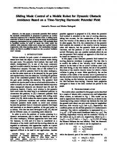
In [9], we presented an analysis for a simplified form of the ROLLERBLADER. A schematic diagram for the simplified robot used to perform the analysis is given in Fig. 3. It was assumed that the robot was planar. A rotary joint and a prismatic joint were used to actuate the two degrees of freedom that allowed the rollerblade to move on the ground plane. The rollerblades were restricted to be always in contact with the ground, i.e. the legs could not be picked up off the ground. The analysis was carried out using the concepts of Lagrangian reduction [10]. In this section, we will extend the analysis to the case where only one rollerblade is on the ground. We will also examine the effects of contact transitions when one leg is brought into or out of contact with the ground. Simulation and experimental results for implementation of gaits on the robot are presented in Section IV. A. ROLLERBLADER configuration with one leg on the ground Our main aim here is to examine the dynamics of the robot configuration with one leg on the ground. We will use the simplified planar version (Fig. 3) of the ROLLERBLADER for analysis. We choose � !#"� %$& (') +*&�� (,-�� %*-� .,.�0/21 to represent the configuration of the system where #"� %$3/ is the position of the central platform in a inertial reference frame, ' is the orientation of the robot in the inertial reference frame, #*&�� %*-�0/ denotes the angular position of links 1 and 2 with respect to the central platform, +, � ., � / are the extensions of links 1 and 2. Let the mass and rotational inertia of the central platform and 576 respectively. Let each link have of the robot be 4 rotational inertial 578 . The mass of the link is assumed to be negligible. Each rollerblade has mass 9 , but is assumed to have no rotational inertia. Further, each rollerblade is fixed perpendicular to the leg, i.e. the angles :&� and :-� in Fig. 3 are fixed at 90 degrees. Note that this is true for our prototype as well. We assume, for simplicity, that the rollerblades can be picked up instantaneously by using an appropriate mechanism at the end of the leg. Thus, the robot is still planar and the legs move in a plane parallel to the ground plane. However, when the rollerblades are picked up the nonholonomic constraint corresponding to that particular rollerblade will be absent and the leg can move freely. Let ;< #"� %$& ('�/>=@?BA�C��/ and DE #*F�G .,0�� %*-�� (,H�0/ denote the group and shape variables for the robot. Let IJ KI7L- %I7MN %I7O�/ denote the body velocity of the robot and let P represent the Lagrangian for the robot. A detailed expression for the Lagrangian and proof of its invariance to the left group action are given in [9]. Consider the configuration of the robot with rollerblade 1 off the ground and rollerblade 2 in contact with the ground. The nonholonomic constraint acting on the robot at rollerblade 2 can be written as a one-form:
Q R� S �UTWVKX3+'B�Y*0�0/+,�"��[Z.\ T]+'B�Y*0�0/+,($^�`_0TaVbXc#*0�0/+,�'��d,N,H��� (1)
R
φ1 (x1, y1) y
γ1 y
Every vector I v =� R must be in both the fiber distribution R and the constraint distribution. Thus, we can write I v in terms of the basis elements for u R and R .
x b
d1
vI R � �� �}�� } � �� " $ Rv � � � I ��B�I v �����I v � ���GI v ��
θ
(x, y)
d2
γ2
φ2
(x2, y2) x
Fig. used for analysis. egfihkj03.h#l)mSimplified planar version of the egn0oahkRpNOLLERBLADER oqh#n�r�h#p�rqm are and are the shape variables. os rs the group variables r and are fixed at t .
The constraint distribution u R is given by the kernel of the one-forms given above. u R represents the kinematic motions possible for the system. A basis for the distribution can be written as:
{ I v� U w xy zxy zxy zxy zxy H{7 zx |� %I v� zxy zxy zxy zxy zxy H{ TWVKX3#*0�`�}'�/ I v� ~w Z(\ T7 *0�G�c'N/+ zTWVKX3 *-�G�c'N/% zxy zxy zxy zxy zx |� %I v ~w xi Wxi Wxi ]{] Wxi zxy zx |� I v w xi zxy zxy zxy H{7 zxy zx |� %I�v Uwgi�W�� (i��� H{] Wxi Wxi Wxi Wx)|�� (2) where,
i�a�W
�,H�&Z.\)T7K*-����'N/b��_0Z(\ TF' (i�C�� ��,H�FTWVKX3#*0����'N/K�c_0TaVbX' � (3) Note that I v and I v represent unconstrained motion of leg 1 since rollerblade 1 is not on the ground. B. Reduction We will now use the process of Lagrangian reduction which leads to simplified equations of motion, allowing us to write them in a lower-dimensional space. It also provides insight into the geometry of the system.The application of this approach to a planar version of the ROLLERBLADER with both rollerblades on the ground is also presented in [9]. C. Constrained Fiber Distribution In the presence of nonholonomic constraints there may exist one or more momenta along the unconstrained directions. The evolution of this momentum vector, referred to as the generalized momentum, is governed by a generalized momentum equation (first derived in [10]). The unconstrained directions are represented by the constrained fiber distribution( R ) which is defined as the intersection of the constraint distribution u R and the fiber distribution R . The fiber distribution contains all the infinitesimal motions of the system that do not alter the shape of the system. The fiber distribution can be written as
R sp
"
$
'
�
'
(4)
I v �� I v �
(5)
Using Eq. 4, Eq. 5 and the basis for the constraint distribution given by Eq. 2, we find that R is two-dimensional. This essentially means that there are two unconstrained directions for the fiber variables. As we shall see shortly, there are also two generalized momenta, each associated with one of the unconstrained directions. Since R is two dimensional, we can write: R R (6) R span #I v /z�� H#I v /C� �
R R KI v z/ � and KI v C/ � are given by: R v KI /z� i �W� �i�C� " R KI v /k�� ] �]� �]�W� "
�}-��
$ $
�}H�a�
' '
(7)
�
(8)
where
i�C�� {7 (]�]� Z(\ T]#*-�`�'N/+ (H�a� }TWVKX3#*0�`�}'�/+ (]�a� xy� (9) and �a� and �C� are given by Eq. 3. The generalized momentum term for the ROLLERBLADER with both rollerblades on the ground represents a scaled version of its angular momentum [9]. With one rollerblade off the ground, two generalized momenta terms are required to describe the dynamics of the configuration. The first term, denoted by &� , is a scaled version of the linear momentum of the robot in a direction perpendicular to the sole nonholonomic constraint acting on the robot, i.e. in the direction of rolling of the rollerblade on the ground. The second term, denoted by N� , represents the (scaled) angular momentum of the robot about the point of contact of rollerblade 2 with the ground. The generalized momentum, - , is given by
R P i` � I v �a
% {] W�i� where summation over the index is implied.
(10)
Using Noether’s theorem [1], the generalized momentum equation specifying the evolution of the momentum can be written as
,(- ,� Here, is
P � �a
R ,-#I 2/ ,(
vR v �7W#I / % {] W�i�
(11)
the one-form of the input torques and forces. For the ROLLERBLADER, this is given as kxy zxy zxy %7)q (.7q +]q ) (.a �/21 where 77q .()q %]q and .a are the input torques/forces corresponding to the *F�G .,0�� %*-� and ,H� ]¡g¢(£¤¥ degrees of freedom respectively. The expression for q¦ v is given by:
R ,-#I / ,(
� � � � � � 3 $ / �§ � �} � "�/ � � � (12) v ~ �� } " $ ' �
(More details on the derivation of this expression can be found in [9] and [2].) Eq. 10 and Eq. 1 give a set of three equations that can be solved to obtain a connection. The connection relates the body velocity (I ) of the robot to the shape inputs for the robot:
� I¨ ��©ª#D�/ D �>&«5 ¬ � ��
(13)
While was a scalar for the case of both rollerblades on the ground, it is now a 2 dimensional vector. Two separate momentum equations given by Eq. 11 give the evolution of ^� and N� over time. We can further exploit the invariance of Eq. 11 to the left group action and use the expression for I from Eq. 13 to rewrite Eq. 11 as:
� { � � � S D 1B
¯ ® ¯ ® #D�/ D � 1� 8 ¯ ® #D�/ D � 1B 8q8N#D�/#Y� 3 « �
(14)
Thus, the evolution of the momentum can be written in a form that involves R only the shape inputs and . « is the projection of along I v . Since has no components along the fiber directions, this projection yields a zero vector. The connection and the momentum equations can also be used to reduce the shape dynamics to a reduced shape-momentum space. Thus, the shape dynamics can be rewritten as:
� ² � ³ � 4° ±D � D 1 « KD�/ D � « #D Dy% &/� ��� « #D�/�
(one rollerblade in contact with ground)
(15)
A similar analysis can be carried out and the appropriate equations derived for the case where rollerblade 2 is picked up off the ground. The analysis for the case where both legs are on the ground has been presented earlier in [9]. The set of equations 13, 14 and 15 defines the complete dynamics of the system. A process of Reconstruction can be used to recover the fiber variables. D. Contact Transitions We will now examine the effects of transition on the system. Each time a leg is placed back on the ground an additional nonholonomic constraint acts on the robot. Each time a leg is picked up, one of the nonholonomic constraints acting on the robot disappears. When the robot transitions from one configuration to another, the generalized momentum needs to be transferred correctly from one basis to another. Fig. 4 depicts the effect of transitions on the system. With the addition of a constraint, the number of unconstrained directions goes down by one while with the removal of a constraint it goes up by one. Thus, the number of generalized momenta required to describe the dynamics of the system changes with every transition. There are two types of transitions, (1): a rollerblade comes into contact with the ground and the number of generalized momenta goes down by one, and (2): a rollerblade goes out of contact with the ground and the number of generalized momenta increases by one. We will examine the two cases separately. The case of a rollerblade coming into contact with the ground will in general be accompanied by some loss of energy. This is because the system loses momentum in the
(both rollerblades in contact with ground) Fig. 4. Transitions between configurations with one and two rollerblades in contact with the ground. ´�µ is two dimensional or one-dimensional.
direction of the new constraint. Thus, the only momentum that is now present will be in the new unconstrained direction(s) corresponding to the new configuration of the robot. We state this observation in the following form: When transitioning from one basis to another, the new generalized momentum in a particular direction is given by the projections of the generalized momenta before transition on the new unconstrained direction. This rule can be stated in a more formal manner. Let #-W/C¶ denote the th generalized momentum, R just after a rollerblade has been put down, in a direction #I v /2 . (We will use the � subscript to denote quantities just after transition and the � subscript to denote quantities just before transition). Let · ¸ denote the size of the configuration space for the robot. Then,
º
KiW/k¶¹
R » P � » KI v / � »¼ � � ¬
(16)
The case of a rollerblade going out of contact with the ground results in the addition of a new unconstrained direction for the system. Thus, the momentum of the system gets distributed among the new set of directions. This effect can be modeled in a manner similar to Eq. 16. For the specific case of the ROLLERBLADER, if ^� and N� denote the two generalized momenta for the robot configuration with only one leg in contact with the ground, we have (after one leg is picked up):
º
º R » R » P P � » #I v / � � » #I v / � � N�] (17) »¼ � � ¬ »½¼ � � ¬ R R KI v z/ � and #I v /C� are given by Eq. 7 and Eq. 8. Equation 17 ^�W
defines the initial conditions for the two generalized momenta needed for the configuration with only one leg on the ground. They can now be used along with the shape inputs in the new configuration to solve Eq. 13. IV. G AIT GENERATION -
SIMULATION AND EXPERIMENTS
In deriving gaits for the ROLLERBLADER, we were inspired in part by human rollerblading motion and walking. For simplicity, we assumed that we have direct control over the shape inputs and are able to drive them directly. This is equivalent to assuming the motors are controlled by a feedback controller that cancels the dynamics in Eq. 15 allowing the
0
LEFT LEG RESET
RIGHT LEG COAST
COAST
PUSH
PUSH
RESET
−0.2 −1
0 −0.5
COAST
0.1 o
0
x 0
CYCLE TIME
0.2
40 0.5
y
0.3
1
1
0.4
(b) G AIT 1: Leg Motion
(a) Phasing of legs for GAIT 1.
0.8
0.8
0.7
0.6
0.6 0.5
y (m)
y (m)
0.4
0
0.3 0.2 0.1
−0.2
0
−0.4
−0.1 −0.2
−0.6 0
0.5
1
x (m)
1.5
0
2
(c) Simulated trajectory from left to right for G AIT 1.
0.2
0.4
0.6
0.8
x (m)
1
1.2
(d) Experimental trajectory from left to right for G AIT 1.
Fig. 5. G AIT 1 0.3
0.4 0.2
0.3 0.1
0.2
0
θ
A. Type 1 gaits In Type 1 gaits, the legs are picked up and reset to their original starting position. It is easy to see that we need to push off against the nonholonomic constraint to achieve motion of the system. Hence, the gaits that we tried were simple gaits where each leg does one of three motions: COAST, PUSH, RETURN. In the COAST part of the motion, the leg stays at a constant relative position with respect to the body. In the PUSH part of the motion, the leg pushes off in a direction parallel to the constraint. The RETURN part involves picking the leg off the ground and returning the leg to a new position after the end of a PUSH. GAIT 1 The first gait (labeled GAIT 1) is represented in Fig. 5(a) by a timing diagram that shows the relative time that the leg spends in each part of the gait. It can be seen that the duty factor (the fraction of a cycle that the rollerblade is on the ground) for this gait is 0.75. The two legs are phased 0.5 cycles apart from each other. The motion of the leg is depicted in Fig. 5(b). The blue (solid) plot is the trajectory of the end point of the leg. The green plane represents the horizontal plane containing the axis of Joint 2 of the robot. The dashed lines indicate the initial position of the leg. The simulated motion of the robot for this gait is shown in Fig. 5(c) and the experimental trajectory is shown in Fig. 5(d). The significant drift in the positive $ direction in the experimental plot is caused by asymmetry of the prototype due to unequal weight distribution and a weaker motor on one of the legs. Lack of significant undulation in the experimental trajectory is partly caused by slipping of the rollerblades which prevented them from executing the PUSH phase effectively. GAIT 2 The second gait (labeled as GAIT 2) is similar to GAIT 1 except that the duty cycle for GAIT 2 is 0.5, i.e. each leg � spends only � of the gait cycle on the ground. The legs come into contact with the ground alternately. Thus, in this case there is no COAST part in the gait cycle. Experimental results for this gait are presented in Fig. 6. The undulations in the trajectory are more pronounced in this case because of the much higher stroke length than in GAIT 1: each leg pushes for 50% of the gait cycle as compared to only 25% of the gait cycle for G AIT 1(although slipping does occur in both cases, the net effect is a doubling of stroke length for GAIT 2).
z 0.2
y (m)
direct control of D�#H/ . In the experimental prototype, the servos give us direct control of the joint angles. Experimental data was obtained using an overhead camera running at approximately 10 Hz. The trajectory of the robot was found by tracking the motion of a bright orange square marker attached to the robot. The orientation of the robot was recovered from the orientation of one of the edges of the square marker. The maximum error in tracking the #"� %$F/ position of the robot was 2.5 cm.
0.1
−0.1
0
−0.2 −0.3
−0.1
−0.4
−0.2 0
0.1
0.2
0.3
0.4
0.5
0.6
0.7
0.8
−0.5 0
2
4
x (m)
6
8
10
12
14
t
(a) Experimental trajectory of ROLLERBLADER from left to right for GAIT 2.
l
(b) (radians) vs. ¾ (s).
Fig. 6. G AIT 2
problem. We examined the use of sinusoidal inputs to drive the robot in [9]. We will now describe these gaits in brief and present new experimental results obtained using these gaits. Symmetric gait The simplest possible gait that can be used is the one where the motions of the two legs are symmetric with respect to the longitudinal axis of symmetry (" axis of the body fixed frame see Fig. 3). We call such a gait, where * � ��[* � and , � , � , a symmetric gait. The symmetric gait generates motion only in the forward direction. The inputs are specified as sinusoids:
�7Â& �]Â& �c:i)�/% %*F�W F*F�ÁÀW�y*F�26yTWVKX3 à �c:y7�/+ 7 ) �7Â^ �7Â& ,H�] ¿,H�GÀW�c,H�G6iTWVKX3 à �c:ya �/+ %*-�] F*-�qÀW��*0�G6iTaVbXc à ��:iq �/+� (18) q q where +,-�ÁÀB Ä,H�qÀ[ Sxi� Å Æ)Çy %*-�GÀ[ ¨x�/ , +,0�Á6c Ä,.�G6c Sxi� x�¸qÇy %*-�G6c B. Type 2 gaits inputs, +:i)- �[*F�Á6� �xi� Å�/ are the amplitudes of the sinusoidal �qÈ .:iq S �GÈ (:y7 xy (:iq U x�/ and à 7 à q S à 7 The generation of gaits for the ROLLERBLADER in the � Ã� configuration with both legs on the ground is a complex q d É{)/ are phase offsets and time periods respectively for ,-�a ¿,0�ÁÀW��,-�26iTaVbXc Ã
the inputs. Fig. 7 shows simulated and experimental motion of the PSfrag replacements PSfrag replacements robot for a symmetric gait. Note: a closer investigation (not Ð shown) of Fig. 7(a) reveals that the forward velocity, I]L , is not constant. Ï Anti-symmetric gait An anti-symmetric gait is a gait with K*F�§ Ê*-�� (,-�§ Ë,H�0/ , i.e the legs move in-phase. An anti(b) Shape varil(a) Simulated l(c) Experimental (radians) vs. ables. (radians) vs. symmetric gait gives rise to pure rotational motion of the robot. ¾ (s). ¾ (s). The inputs for the gait are still given by Eq. 18 but now Fig. 8. Simulated and experimental anti-symmetric gait. *&�Á6} Ì*-�G6 Êxy� Å . All the other parameters have the same values as in the forward motion gait. Fig. 8 shows simulated Given a trajectory to follow we would like to be able to and experimental results. The spike in the value of ' at the automatically generate a gait that takes the robot along this end of the gait is because ' wraps around from �¹Â to  . trajectory. This would allow us to generate motion plans for the robot or control it using a joystick-like interface. In [11], an optimal control method was used to generate gaits for the PSfrag replacements Snakeboard and is potentially applicable to our system as well. replacements Í A method of achieving point to point motion is to concatenate the Type 2 gaits presented here to move from point Î to point. However, this results in the robot coming to rest each time it transitions between gaits. In contrast, human f rollerbladers frequently use the concept of coasting, i.e. they (a) (m) vs. ¾ (s). (b) Shape vari(c) Experimental ables trajectory. build up momentum for some time and then steer themselves. Fig. 7. Simulated and experimental symmetric gait for the ROLLERBLADER . We would like to be able to achieve the same effect, both in simulations and experiments. This would require the design of C. Discussion of experimental results. gaits that build up momentum or brake the robot. Acknowledgement The support of NSF grant IIS02-22927 Several practical problems arose in the experimental imis gratefully acknowledged. plementation of the gaits. The most important was the effect of friction on the robot. The rollerblades do not provide R EFERENCES enough traction in the lateral direction. Thus, the legs of the [1] J. P. Ostrowski, “The mechanics and control of undulatory robotic robot were continuously slipping, violating the nonholonomic locomotion,” Ph.D. dissertation, California Institute of Technology, constraints. This limited the ability of the legs to push off Pasadena, CA, 1995. [2] P. S. Krishnaprasad and D. P. Tsakiris, “G-snakes: Nonholonomic the nonholonomic constraints. Thus, the robot was not able kinematic chains on lie groups,” in Proc. ÑGÑ7ÒWÓ IEEE Conf. on Decision to match the simulated motion. Increasing the weight of the and Control, Buena Vista, FL, 1994. robot will improve friction at the blades but will also increase [3] ——, “Oscillations, SE(2)-Snakes and Motion Control: A Study of the Roller Racer,” Center for Dynamics and Control of Smart Structures friction at the casters. The requirement for a central platform (CDCSS), University of Maryland, College Park, Tech. Rep., 1998. supported by omnidirectional casters can only be removed by [4] S. Hirose and A. Morishima, “Design and control of a mobile robot with developing a dynamically stable rollerblader. an articulated body,” The International Journal of Robotics Research, 0
0.5
−2
0.4
4
d
1
3 2
0.3
−4
1
0.2 0.1
−8
1.6
0.5
1.4
0.4
−2 −3
−0.2
0.2
0.4
0.6
0.8
1
−0.3 0
0
−1
0.2
0.4
t
0.6
0.8
1
−4 0
5
10
15
20
25
30
35
40
t
0.6
d
1
0.4
0.3
1.2
0.2
0.2
y (m)
1
0.1
γ
0.8
0
0.6
0
1
−0.1
0.4
−0.2
−0.2
0.2
0 0
1
−0.1
−12
−14 0
γ
0
−10
θ
−6
−0.4
−0.3
0.2
0.4
t
0.6
0.8
1
−0.4 0
0.2
0.4
0.6
0.8
1
0
0.2
0.4
0.6
0.8
1
1.2
1.4
x (m)
V. C ONCLUSION AND FUTURE WORK In this paper, we have presented the design for a ROLLERBLADER robot. Analysis of the robot was carried out using the method of Lagrangian reduction. Contact transitions were handled using appropriate momentum transfer equations. Simulation results were presented for two types of gaits. The gaits were then implemented on the prototype of the robot. The gaits include a novel gait that turns the robot in place with both rollerblades on the ground throughout the gait and two gaits motivated by human rollerblading motion. We plan to improve the design of our prototype by reducing the weight of the legs and adding springs to help the servos lift up the legs. We plan to add an additional degree of freedom to the rollerblades by actuating the angles :F� and :0� (Fig. 3). Another line of future work we are planning to explore is the design of a dynamically stable rollerblading robot where dynamic balance issues would play a very big role.
vol. 9(2), pp. 99–114, 1990. [5] D. Rus and M. Vona, “Self-reconfiguration planning with compressible unit modules,” in Proceedings of the IEEE International Conference on Robotics and Automation, Detroit, 1999. [6] R. Altendorfer, E. Z. Moore, H. Komsuoglu, M. Buehler, H. B. B. Jr., D. McMordie, U. Saranli, R. Full, and D. E. Koditschek, “Rhex: A biologically inspired hexapod runner,” Autonomous Robots, vol. 11, pp. 207–213, 2001. [7] S. Hirose and H. Takeuchi, “Study on Roller-Walker (Basic Characteristics and its Control),” in Proc. IEEE Int. Conf. Robotics and Automation, Minneapolis, 1996, pp. 3265–3270. [8] G. Endo and S. Hirose, “Study on Roller-Walker : Multi-mode steering control and self-contained locomotion,” in Proc. IEEE Int. Conf. Robotics and Automation, San Francisco, April 2000, pp. 2808–2814. [9] S. Chitta and V. Kumar, “Dynamics and generation of gaits for a planar rollerblader,” in Proc. IEEE Intl. Conf. on Intelligent Robots and Systems, Las Vegas, October 2003. [10] A. M. Bloch, P. S. Krishnaprasad, J. E. Marsden, and R. M. Murray, “Nonholonomic mechanical systems with symmetry,” Archive for Rational Mechanics and Analysis, vol. 136(1), pp. 21–99, 1996. [11] J. P. Ostrowski, J. P. Desai, and V. Kumar, “Optimal gait selection for nonholonomic locomotion systems,” The International Journal of Robotics Research, vol. 19(3), pp. 1–13, March 2000.