NORTHWESTERN UNIVERSITY. Design and Optimization of Architectures for
Data Intensive Computing. A DISSERTATION. SUBMITTED TO THE GRADUATE
...
NORTHWESTERN UNIVERSITY
Design and Optimization of Architectures for Data Intensive Computing
A DISSERTATION SUBMITTED TO THE GRADUATE SCHOOL IN PARTIAL FULFILLMENT OF THE REQUIREMENTS for the degree DOCTOR OF PHILOSOPHY
Field of Electrical and Computer Engineering
By Jayaprakash Pisharath
EVANSTON, ILLINOIS December 2005
c Copyright by Jayaprakash Pisharath 2005
All Rights Reserved
ii
ABSTRACT
Design and Optimization of Architectures for Data Intensive Computing
Jayaprakash Pisharath
Computer technology in recent years is propelled by new hardware designs, advanced software features and multitudinous user demands. Due to this, the data collected and managed by applications is also abundant. Today’s “connect anytime and anywhere” society based on the use of advanced digital technologies has increased the expectations of users. Data access is expected to be quick, highly reliable and fast. Future systems are expected to even more data centric and compute intensive. This fact is used as a motivation in this research work to propose new techniques and optimizations that enable high speed access to data. A three-tier data driven approach is taken to propose new architectural designs and techniques. The three perspectives of data that is used are streaming data, structured databases and new-age massive datasets (could be structured or unstructured). iii
Streaming data is widely popular and is still emerging. In this work, new scheduling and resource allocation strategies are proposed for such stream data systems. Both performance and energy improve dramatically when the proposed schemes are deployed in existing heterogeneous systems. Also, a new framework of analysis is proposed to comprehensively study the performance and energy consumption of such high performance systems. The next focus area of this work is modern database systems. Storage technology has evolved significantly in the recent years. In this study, modern memory technology is used as a motivation to tune and adapt modern DBMS to modern storage technology. First, dynamic hardware management schemes are proposed. Secondly, the query optimizer is also modified to reflect the change in the storage architectures. Other emerging storage paradigms are also considered in this work. With data growing at alarming proportions, data mining is emerging to be an excellent tool to automatically extract useful information from such large datasets. The growth of data, the advancements in data mining tools, and the user expectations are totally incongruent to the improvements in the performance of general purpose computing systems. To alleviate this, a new data mining system is designed that achieves massive speeds that can never be achieved using traditional high performance techniques.
iv
Acknowledgements I express my sincere gratitude to everyone that helped me in accomplishing my doctoral research work. I am grateful to my research advisor, Alok Choudhary, for his constant guidance and extensive feedback. This work was supported in part by DOE under contract 28264, DOE’s SCiDAC program (Scientific Data Management Center) award number DE-FC02-01ER25485, NSF’s NGS program under grant CNS-0406341, NSF/DARPA ST-HEC program under grant CCF-0444405, and in part by Intel Corporation. I would like to thank my committee members Lawrence Henschen and Peter Scheuermann for their valuable feedback. I am indebted to Mahmut Kandemir at the Pennsylvania State University for providing me priceless help and advice with the database research work. I am grateful to my dad Jayarajan Pisharath and mom Bhagavathi Pisharath for their encouragement and moral support through all these years in my life, and also for providing me the best possible level of education and knowledge. Also, I would like to thank my friends, especially the gutter gang, for those lighter moments during my doctoral study at Northwestern. Thanks are due to my fellow researchers at the Center for Ultra Scale Computing and Information Security at Northwestern University for teaming with me in realizing my research goals.
v
Contents ABSTRACT
iii
Acknowledgements
v
List of Tables
x
List of Figures
xii
Chapter 1.
Introduction
1
Chapter 2.
Background and Related Work
10
2.1.
Architecture Optimizations
10
2.2.
Performance-Energy Tradeoff Frameworks and Tools
14
2.3.
Modern Databases
17
2.4.
Data Layouts for Emerging Storage Devices
22
2.5.
Data Mining Application Analysis and System Design
23
Chapter 3.
Performance-Energy Optimization Techniques for Multiprocessor Systems
26
3.1.
Multiprocessor and Heterogeneous Streaming Systems
26
3.2.
Approach
28 vi
3.3.
Heterogeneous Platform
29
3.4.
Methodology
34
3.5.
Performance-Energy Analysis
36
3.6.
Overall Observations and Shortcomings of Traditional Metrics
40
Chapter 4.
Energy-Resource Efficiency Framework
42
4.1.
ERE Framework
43
4.2.
Analysis Setup
47
4.3.
Evaluation of ERE Framework
48
4.4.
Extension of ERE Framework
56
4.5.
Summary
57
Chapter 5.
Energy Management Techniques for Memory Resident Databases
59
5.1.
Memory Resident Databases
59
5.2.
System Architecture
63
5.3.
Power Management Schemes
71
5.4.
Experimental Evaluation of Memory Management Schemes
78
5.5.
Summary
93
Chapter 6.
Data-Driven Query Optimizations for Memory Resident Databases
94
6.1.
Data Windowing
95
6.2.
Query Restructuring
99
6.3.
Experimental Evaluation
105
6.4.
Summary
112 vii
Chapter 7.
Database Layouts for MEMS-Based Storage Systems
114
7.1.
MEMS Device and Characteristics
116
7.2.
Data Layouts for a Single Table
118
7.3.
Data Layouts for Multiple Tables
124
7.4.
I/O Performance Evaluation of Layouts
129
7.5.
Discussion
140
7.6.
Summary
141
Chapter 8.
Workload Characterization Framework for Data Mining Applications 144
8.1.
Methodology
145
8.2.
Data Mining Workload
148
8.3.
Evaluation and Analysis Framework
156
8.4.
Characteristics of Data Mining Applications
165
8.5.
Summary
181
Chapter 9.
Architectural Acceleration of Data Mining Kernels
184
9.1.
Data Mining Applications Mix
186
9.2.
Workload Characteristics
187
9.3.
Architectural Exploration
192
9.4.
Evaluation of Acceleration
200
9.5.
Summary
207
Chapter 10.
Conclusion
209 viii
References
212
ix
List of Tables 3.1
Typical power consumption of MPC7410
32
3.2
Typical power consumption of MSC8101
32
3.3
Software setup
33
3.4
Benchmarks used in evaluating the heterogeneous setup
37
4.1
Interpretation of ERE framework values
46
5.1
The two classes of queries considered for the experiments
81
5.2
SQL for organizer queries
83
6.1
Scenarios for organizer queries
106
6.2
Scenarios for TPC-H queries
106
7.1
Device parameters used in experiments
130
7.2
Summary of layout performance
142
8.1
Algorithms used in the study and their descriptions
151
8.2
Dataset for classification and ARM applications
161
8.3
SEMPHY datasets and their characteristics
162
x
8.4
Comparison of data mining application with other benchmark applications
169
8.5
Top kernels of data mining applications
173
9.1
Algorithms used in this study and their descriptions
187
9.2
Kernels of the applications
191
9.3
Architectural performance of the kernels
191
9.4
Datasets used in the experiments
203
xi
List of Figures 3.1
Heterogeneous architecture
29
3.2
Base power consumption of the board.
34
3.3
Power, execution time, energy and energy-delay product for art
38
3.4
Power, execution time, energy and energy-delay product for g721
38
3.5
Power, execution time, energy and energy-delay product for bzip2
38
3.6
Power, execution time, energy and energy-delay product for jpeg
39
3.7
Power, execution time, energy and energy-delay product for pegwit
39
4.1
Design of ERE framework
44
4.2
ERE framework for scalable applications
50
4.3
ERE framework for pegwit
53
4.4
ERE framework for multi-stream applications
55
5.1
Energy consumption of a memory resident database
63
5.2
DBMS architecture
64
5.3
Banked memory architecture
66
5.4
Available operating modes and their resynchronization costs
68
xii
5.5
Dynamic threshold scheme
72
5.6
Example application of the query-directed scheme
79
5.7
Energy consumption of hardware and software-directed modes
85
5.8
Low power mode utilization
87
5.9
Performance overheads
88
5.10
Impact of bank size
90
5.11
Threshold sensitivity
92
6.1
Data windowing
100
6.2
Reorganizing operations within a query to optimize for energy
103
6.3
Grouping schedule list from multiple queries
104
6.4
Query restructuring
105
6.5
Energy improvements from query restructuring
108
6.6
Inter-query benefits
108
6.7
Energy savings from query restructuring
109
6.8
Performance improvement from query restructuring
111
6.9
Overall performance of query restructuring
112
7.1
MEMS device
116
7.2
MEMS device with respect to traditional terminology
117
7.3
Row layout for MEMS
119 xiii
7.4
Column layout for MEMS
121
7.5
Object layout for MEMS
123
7.6
Row-interleaved layout for MEMS
125
7.7
Column-interleaved layout for MEMS
126
7.8
Row-fill layout for MEMS
127
7.9
Column-fill layout for MEMS
128
7.10
Object-fill layout for MEMS
129
7.11
Experimental MEMS framework
131
7.12
I/O service times
132
7.13
Cache performance
138
8.1
Evaluation perspectives
148
8.2
Data mining taxonomy
149
8.3
Evaluation and analysis framework
157
8.4
Analysis flow
164
8.5
Measures of interest for evaluation and analysis
165
8.6
Automated classification of data mining, SPEC INT, SPEC FP, MediaBench and TPC-H benchmark applications
168
8.7
Multi-phased operations seen in data mining
171
8.8
Processor scalability of data mining applications
179
xiv
8.9
Data scalability of data mining applications
180
9.1
Design goals
185
9.2
Data mining system
194
9.3
Hardware logics for distance and min kernels
199
9.4
Hardware logic for the density calculation kernel
200
9.5
Applications for acceleration and their logics
201
9.6
Performance of accelerated kernels
204
9.7
Hardware sensitivity analysis of kernels
205
9.8
Application speedups
206
xv
CHAPTER 1
Introduction New technology has also unleashed its own flood of data. With the establishment of an extensive network infrastructure, including the Internet, corporate Intranets and virtual private networks, a reliance on electronic data to conduct both front and back office business is mounting. For instance, one of the leading business chains, Walmart, gathers information in the order of about 20 million customer transactions per day from all its establishments. Such high volume data collection is enabled through sophisticated data collection infrastructure, which includes both software tools and human resources. The gathered information is in turn used by Walmart to provide customized services (e.g., in Customer Relationship Management). But this piling up of information also brings forth brand new challenges in the computing world; in Walmart’s case, massive data processing capabilities are needed in systems in order to extract meaningful information (like customer purchase patterns) from such a flood of transactions in a timely manner. In the mass storage industry, technology advancements have consistently delivered reduced cost per megabyte, increased storage capacity, and improved storage mechanisms. Thanks to these developments in storage technologies, today, there are gigabytes of photos, music, video and other personal data stored on systems. Personal computing paradigm has been steadily changing. A digital transformation is underway; anything
1
2
that can be digitally recorded is being recorded. Researchers assert that for each person on the planet roughly 800 megabytes of data are recorded annually. And the amount of that data is doubling every 18-24 months [Cor05]. Between 1999 and 2002 new data stored on electronic media grew by 30 percent, according to a recent report by the University of California, Berkeley. The same study says that print, film, magnetic, and optical storage media produced about 5 exabytes of new information in 2002 – that’s equal to nearly half a million new Libraries of Congress. In the near future, there will be terabytes of digital data that will require teraflops of processing power to manage, analyze, and synthesize meaningful information. Improvements in storage and network technologies have also impacted the scientific community. Until a few decades ago, investigative methods in most scientific and engineering disciplines were either empirical or theoretical. Recently, computational science has emerged as a major branch in these disciplines. It is not uncommon to see collecting vast amounts of data to make forecasts and intelligent decisions about future directions. The National Science Foundation (NSF) spends more than 170 million dollars every project term to enable the collection and analysis of data pertaining to weather prediction. The world’s largest commercial databases are approaching the 50TB mark, whereas the database sizes on hybrid systems are approaching the PB mark. Some of these large databases are growing by a factor of 20 every year. This does not even include the amount of data made available by millions of users on the Internet. In addition to the increasing amount of available data, there are two other major factors that make the
3
problem of information extraction particularly complex. The first challenge is the need for increasingly complicated algorithms to analyze and extract meaningful information from the large data sets. Second, in many cases, such analysis needs to be done in real time to reap the actual benefits. For instance, a security expert would strive for real-time analysis of the streaming video and audio data in conjunction. Managing and performing run-time analysis on such data sets is appearing to be the next big challenge in computing. As the data trends suggest, there is an increasing need for automated data analysis tools to extract the required information and to locate the necessary data objects. There are numerous commercial, research and scientific tools that have been proposed, developed and currently being used. Researchers at the Jet Propulsion Laboratory apply neural-network based learning techniques to the images collected from Venus in order to identify volcanoes. Every computing community faces the need to develop new tools every day. Recently, the Department of Energy’s Oak Ridge and Pacific Northwest national laboratories have teamed up to learn about new aspects of biological research through the use of data-intensive computing capabilities. They are planning to develop tools that enable such capabilities. Such data intensive applications are characteristically different from traditional IT applications, which are targeted by current hardware and software systems. Just as graphics and multimedia applications have had tremendous impact on processors and systems, these data intensive data mining applications will have tremendous impact on future systems. Besides this fact, more sophisticated and
4
data-intensive application systems have emerged in the past from significant advances in processing power and performance. As sheer volume of data is rising rapidly, the level of complexity in data type and in data analysis tools also arise. The deluge of data must not only be stored somewhere, but also be managed and processed efficiently. On one hand, it requires that algorithms and software is efficiently optimized. While on the other hand, even computing systems have to be redesigned and customized to efficiently host these data intensive applications. This requires innovative and “smarter” computing architectures. Such architectural innovations should strive to achieve new performance levels in data intensive computing on a scale not previously seen. Such innovations would enable high performance computing in the new era of digital transformations. This forms the core goal of this thesis work. Future systems are bound to be data-intensive, and require significant design enhancements to alleviate several drawbacks. This research work addresses a section of these design challenges. It focuses on diverse topics in system design. The designs and optimizations proposed in this thesis take a three tier approach. This is basically a datadriven approach rather than control driven. There are three different kinds of data that are processed in current systems and which is bound to be seen in future systems. This includes streaming data, resident databases and massive datasets. One of the diverse data types existing today is streaming data. It seen in a wide range of systems, ranging from hand held devices to high performance equipment. Features like video, text messaging, audio and voice are not uncommon in new cellphones. On
5
the other hand, streaming data is also seen in multiprocessor heterogeneous systems like communication base stations, switchboards, set-top boxes, sensor network servers and web servers. The first section of the thesis focuses on enabling high performance on such streaming setups. Besides performance, energy consumption is also a crucial issue in the design of such multiprocessor streaming systems. In Chapter 3, an applicationdriven task scheduling scheme is proposed for such systems. This scheme aims to improve the performance and concurrently reduce the energy consumption. The proposed scheme uses stream data as a driving model to optimally partition processor resources, and schedule application tasks. In reality, achieving a good tradeoff between performance and energy consumption is a tedious task since it requires a thorough analysis of the system under consideration, which could be time consuming. Existing analysis tools and frameworks do not take into consideration the streaming nature of data or even the presence of constraints in heterogeneous multiprocessor systems. The existing metrics and measures lack the capabilities of highlighting the real performance and energy improvements in these systems. Chapter 4 addresses this fact and proposes a new analysis framework called Energy-Resource Efficiency (ERE). This framework systematically analyzes the performance, energy consumption and resource-efficiency of a system to highlight the various performance-energy tradeoffs. With a pre-defined performance and energy requirement, the ERE can also be used to find the minimal number of resources needed to achieve that desired configuration.
6
Another prominent data type is databases. Database is typically an organized collection of records having a standardized format and content. Computerized indexes and catalogs are some of the most common types of databases. Simple access schemes are seen in structured address books on hand held devices, whereas online library catalogs carry a complex indexing structure to access the database. Databases have evolved through ages. Access schemes are smarter and well optimized. A lot of optimizations have been done from the algorithmic and query perspectives. As databases are evolving, so is the data storage technology. Modern database techniques do not take into consideration the underlying storage technologies. This work uses this as a motivation to propose database access techniques that take into consideration all of the design factors, namely the databases, the query structures, the access patterns and the underlying storage system. Memory, a core storage component, has evolved in recent years to become more structured and partitioned, providing ample optimization opportunities. Chapter 5 uses this as a motivation to propose memory hardware schemes that smartly take into consideration the database system. That is, the memory tunes itself to the needs of the DBMS, thus enhancing the performance. This is achieved by taking advantage of the multiple modes of operation that are available in current memory systems. Chapter 6 goes one step further and optimizes the DBMS to take into consideration the smart allocation schemes in new storage architectures. Intelligent intra-query and inter-query restructuring schemes are proposed, which optimize queries to adapt to the changing
7
storage technologies of the system. Chapter 7 sets out to find answers to various questions that arise while storing a database in a new storage technology based on MicroElectroMechanical Systems (MEMS). MEMS based storage devices do not use rotating mechanical components like the ones seen in hard disks, and are known for lower cost, higher performance and increased reliability. This thesis proposes a mapping between application (high-level) database layouts and device (low-level) data layouts by taking advantage of the features associated with the underlying MEMS storage device. As already mentioned, data is growing at an exponential rate. Databases are becoming larger by the day, and the paradigm of having structured records and structured query-based access to the database is no longer valid. These days, large datasets are common, data structures are complex, and access schemes are intricate. Sophisticated analysis tools are already in place. Especially, as the data sizes are exponentially increasing, the need to use complicated tools to extract information from the collected data becomes clear. Data mining, an automated method to extract useful information from large datasets, is becoming widely popular. Data mining programs have become essential tools in many domains including marketing, customer relationship management, scoring and risk management, recommendation systems, and fraud detection. In addition, data mining techniques have been adopted by various scientists to analyze the vast amounts of data representing real-world systems. Data mining techniques have been utilized in cosmology simulation, climate modeling, bioinformatics, drug discovery, and intrusion detection.
8
As the amount of data collected increases, there arises a need to utilize even more complicated data mining applications. However, one important obstacle that has to be addressed is the fact that the performance of computer systems is improving at a slower rate compared to the increase in demand for data mining applications. Recent trends suggest that the system performance (data based on memory and I/O bound workloads like TPC-H) has been improving at a rate of 10-15% per year, whereas, the volume of data that is collected doubles every year. Having observed this trend, researchers have focused on efficient implementations of different data mining algorithms. Another approach to address this problem is to develop an understanding of the characteristics of these applications. This information in turn can be utilized during the implementation of the algorithms and the design/setup of the computing systems. Understanding the architectural bottlenecks is essential not only for processor designers to adapt their architectures to data mining applications, but also for programmers to adapt their algorithms to the revised requirements of applications and architectures. In Chapter 8, several widely-used data mining algorithms from many domains are extensively studied by means of a new automated analysis framework. The framework is used to study data mining applications as a workload for future platforms. The workload characterization results are then used to design NU-MineBench, a benchmarking suite containing representative data mining applications. This is a major contribution of this work. The characterization studies proved that data mining applications are very different from traditional applications (including DBMS). Data mining applications have multiple phases of compute and data intensive computations, which are called kernels. These
9
kernels are identified for every data mining application. Some of the kernels are common across data mining applications. Once these kernels are extracted, designing high performance schemes for data mining applications becomes an easy task. This is because kernels contribute to majority of the execution times. Hence, when the kernels are accelerated, the entire application also speeds up. This thesis also extends scalable high performance techniques to these kernels of data mining applications to achieve application speedups. Chapter 9 goes one step further and presents a new data mining system. This new data mining system has a reconfigurable hardware accelerator in addition to the traditional processor. The task of this accelerator is to accelerate the kernels of data mining applications. Kernels of applications are identified using automated analysis tools after extensive workload characterization. The results show that remarkable speedups are achieved when an accelerator based data mining system is used to execute the applications. Such speedups are not seen in traditional systems. The rest of this document is organized as follows. The summary of all related work is presented in Chapter 2. Chapter 3 and Chapter 4 discuss the optimizations for streaming architectures. Chapter 5 discusses the new memory energy management schemes designed for databases. In Chapter 6, new data-driven multiquery optimizations are proposed. These optimizations take into the consideration the database and the storage technology underneath. Chapter 7 proposes new database access layouts for MEMS based storage systems. Workload characterization of data mining applications are covered in Chapter 8. Chapter 9 uses these characterization results to propose a new data mining systems architecture. The thesis work is concluded in Chapter 10.
CHAPTER 2
Background and Related Work This chapter introduces the related work and background for the work presented in this document. This section is organized based on the chapter layout. First, it discusses architecture based techniques to enhance the performance and reduce the energy of data intensive systems. Several metrics and measures for evaluating and assessing system performance and power consumption are also discussed. Following this, the related work in the field of modern databases is then covered. The topics discussed include both hardware and query driven schemes that are proposed by researchers and widely used both in the industry and academia. Well known data layouts for existing and emerging storage architectures are also discussed. The last section covers high performance data mining systems. This includes even the limited data mining application characterization work that has been done in the past.
2.1. Architecture Optimizations 2.1.1. Memory Hierarchy Memory is a very common candidate for low power design. Lebeck et al. proposed a power-aware page allocation scheme for the main memory [LFZE00]. In this work, the different operating modes of RDRAM are exploited to improve the energy-delay 10
11
product. This dynamic scheme forms the basis for the proposed power-aware memory hierarchy. Another approach by Delaluz et al. introduced novel techniques to exploit the low-power operating modes of DRAMs [DKV+ 01]. These techniques include heuristics that use fixed thresholds for detecting idleness and an adaptive threshold that attempts to adjust itself with the dynamics of a program. Significant work has been done on designing low-power caches. An integrated architectural and circuit-level approach by Se-Hyun et. al aims at reducing leakage energy in instruction caches [YPF+ 01]. They introduced DRI i-cache, an i-cache that can dynamically resize and adapt itself to an application’s requirements. Kamble and Ghose proposed architectural techniques to reduce power consumption in on-chip caches, and also provided analytical models for estimating energy dissipation of conventional caches as well as low-power caches [KG97, GK99]. Compiler and hardware-based approaches to reduce cache misses, by Sherwood et al. [SCE99], suggest dynamic reordering of pages in physically addressed caches. In [Alb00], Albonesi proposed an on-demand cache resource allocation policy called selective cache ways. Selective cache ways technique gives the ability to disable a subset of ’ways’ in a set associative cache during periods of modest cache activity, while the full cache may remain operational for more cache-intensive periods. A mechanism called Cache Decay, proposed by Kaxiras and Hu [KH01], exploits generational behavior of caches to reduce cache leakage power. Bahar et al. have studied power-performance tradeoffs for several power/performance sensitive cache configurations, which involve techniques like increasing cache size or associativity and including buffers along side L1 caches [BAM98].
12
Brooks et al. proposed a framework for analysis and optimization of power at the architectural level [BTM00]. Wattch provides a power evaluation methodology within the portable and familiar SimpleScalar [Aus] framework. The proposed model for power estimation is based on the Wattch model. One of the major challenges that the hardware industry faces today is to cope with the immense power requirements of integrated circuits. Most of the studies and proposals for minimizing the power requirements of computing systems are directed towards processors and peripherals. The power consumed by processor cores are decreasing drastically, leaving the memory hierarchy and other external components as the significant bottleneck. For instance, the memory hierarchy could consume up to 50% of the power for memory intensive applications, and the off-chip data bus could consume up to 20% of the power. Hence, there arises a need for optimizations that reduce the power consumption without affecting the performance of the system. This forms the motivation for the work done in [PC02] and [BCPK02]. In [PC02], a power-aware memory hierarchy is proposed. This power-aware memory hierarchy improves the system energy consumption and performance by 50%. A new layer called Energy-Saver Buffers is also introduced between the cache and memory subsystem. In [BCPK02], a new data bus protocol called Power Protocol is proposed. This protocol is very effective in reducing the traffic over the data bus by proposing a data cache called ”value cache” for the bus. As a result of caching, the energy and the performance improves by average 42%. These two work are mentioned here to emphasize the need for new architectural techniques that keep pace with emerging computing
13
requirements and design parameters. Thus, these work form the first layer (architecture) of the multi-layered model considered in this document.
2.1.2. External Data Bus Most of the existing work in bus encoding aims towards improving the performance and effective bandwidth of the bus. For example, Citron and Rudolph have described a technique to encode data on the bus using a table-based approach [CR95]. In this method, they divide a given data item (to be transferred over the bus) into two parts. The lower part is sent without being encoded, while the upper part is encoded using a look-up table (LUT). Their method aims at reducing the size of the data being sent. The upper part of the data is broken into a key, which is used to search the data in the LUT, and a tag, which is used to match the data in the LUT to find if there is a hit. If there is a hit, the data sent over the bus is compacted to y [y=Comp(x)], where x is the original data and the lower d bits of y is the same as the lower d bits of x. On the receiving end, a component called bus expander expands y to original data x [x=Expn(y)]. It follows that x=Expn(Comp(x)). In the recent past, the encoding paradigms for reducing the switching activity on the bus lines have been investigated (e.g., [SB97, MOI96]). Most of the common encoding techniques rely on the well-known spatial locality principle. An analysis of several existing low-power bus encoding techniques such as T0, bus inversion, and mixed encoding has been performed by Fronaciari et al. [FSS99]. Among the different techniques that have been studied for reducing the power dissipation of the address bus, Gray code
14
addressing appears to be a very efficient scheme [MOI96]. Shin, Chac, and Choi have explored a partial bus invert coding technique where they proposed a heuristic to select only portions of the bus to invert for further improving the effectiveness of the bus inversion coding [SCC98]. They have also proposed a combination of bus inversion with transitional signaling for a typical signal processing application. Techniques using look-up tables to compress data have been explored by Bishop and Bahuman who have proposed an adaptive bus coding to reduce bit transition activity by exploiting the repetition of the data [BB01]. Childers and Nakra have studied the effect of reordering the memory bus traffic to reduce power dissipation [CN00]. Yang et al. [YZG00] have proposed the use of a compression cache to compress the data stored in the cache line to at least half their length so that a single cache line can effectively store two cache-lines of data. However, their main objective is to compress the data in the on-chip cache and increase the cache hit rate. Since their approach sends the data across the bus in a compressed form, it also results in a reduction in bus activity. Also, the compression strategies used in this work and in [YZG00] are entirely different. Farrens and Park [FP91] have presented a strategy that caches the higher order portions of address references in a set of dynamically allocated base registers. The bus energy optimization strategy is also similar to the strategy proposed by Yang and Gupta [YZG00].
2.2. Performance-Energy Tradeoff Frameworks and Tools Power optimizations have been proposed for all the kind of systems. A survey of some of the prominent power optimization techniques for generic systems was done by
15
Benini and Micheli [BM00]. An energy-conscious reconfigurable system with DSPs has been explored by Wan et al. [WILR98]. The focus of this work is on the flexibility and the adaptability of reconfigurable processors in a heterogeneous environment. TienChien-Lee et al. developed an instruction-level power model for DSPs and proposed some energy minimization techniques based on this model [TCLTMF97]. Due importance is given to power-performance tradeoffs by all power-aware system architects. In [BMWB00], Brooks et al. used a fast cycle accurate simulator to model power and to derive energy characterizations. Using the simulated data, they perform a detailed power-performance tradeoff study. Yang et al. performed a quantitative study on energy-efficient architectures and developed an integer linear program to model performance-power tradeoffs in such architectures [YGGT02]. By presenting some power evaluation mechanisms in [JM01], Joseph et al. consider a wide range of power-performance tradeoffs in a general purpose CPU. Vijaykrishnan et al. [VKI+ 00] undertook an integrated hardware-software approach to power reduction by applying power optimizations at the compiler level and studying their impact on some of the existing power-aware hardware technologies. They used a simulation-based tool for power estimation.
2.2.1. Evaluation Metrics and Measures Estimation and evaluation of power consumption has become a crucial step in designing efficient computing systems. Significant work has been done on power estimation and evaluation for low-power embedded processors. Researchers have proposed
16
both analytical models and simulation-based methods for estimating power consumption. Kamble and Ghose provided analytical models for estimating energy dissipation of caches [KG97]. In Wattch [BTM00], Brooks et al. propose a framework for analysis and optimization of power at the architectural level. SimplePower [YVKI00] is a cycleaccurate RT level energy estimation tool developed by Ye et al. Cignetti et al. designed a tool for the estimation of energy consumption in PalmOS family of devices [CKE00]. This tool works on a set of empirically derived performance and energy values. These values are measured using a framework consisting of an oscilloscope, a power supply and an IBM workpad. In the work done by Joseph and Martonosi [JM01], the runtime power dissipation of different processor units is estimated. Power is modeled by associating it with a set of performance counters defined in the hardware. The metrics that are used to measure performance-energy tradeoffs typically target uniprocessor architectures. Energy-delay product is a very well known metric used for such studies [HIG94]. Most of the work mentioned in the previous paragraphs use this metric. For low-end systems, even energy-per-operation [BB95] gives a rough estimate of the power-performance behavior. Some of the researchers also use custom frameworks to quantify performance-energy tradeoffs ( [YGGT02] for instance). In [ZS02], Zyuban and Strenski use a mathematical approach to introduce a new metric for representing speed-power tradeoffs. They consider various circuit power implications to design a new variable called hardware intensity, which is used for evaluating issues that affect both circuits and microarchitecture. The above metrics work well when applied to
17
uniprocessor architectures. Heterogeneous and parallel systems require special consideration due to the presence of multiple processing elements. Hence these metrics may not quantify the best available tradeoffs. This thesis work uses this fact as the motivation to develop a new metric called energy-resource efficiency (ERE). 2.3. Modern Databases 2.3.1. Hardware Schemes for Databases In the past, memory has been redesigned, tuned or optimized to suit emerging fields. Need for customized memory structures and allocation strategies form the foundation for such studies. Copeland et al. proposed SafeRAM [CKKS89], a modified DRAM model for safely supporting memory-resident databases alike disk-based systems, and for achieving good performance. In PicoDBMS [PBVB01], Pucheral et al. present techniques for scaling down a database to a smart card. This work also investigates some of the constraints involved in mapping a database to an embedded system, especially memory constraints and the need for a structured data layout. Anciaux et al. [ABP03] explicitly model the lower bound of the memory space that is needed for query execution. Their work focuses on light weight devices like personal organizers, sensor networks, and mobile computers. Boncz et al. show how memory accesses form a major bottleneck during database accesses [BMK99]. In their work, they also suggest a few remedies to alleviate the memory bottleneck. In [WKKS99], Weikum et al. propose a self-tuning memory management system for databases. They propose memory-based techniques that tune data storing and fetching to improve the performance. Bouganim et
18
al. develop a memory-adaptive scheduling technique for queries that perform memoryintensive operations [BKV98]. In their scheme, memory is both statically and dynamically managed based on the input query.
2.3.2. Data-Centric Query Optimizations Memory-resident databases have been studied since a long time back by various researchers. In the past, memory technology bottlenecks have prevented the actual implementation of these databases. Currently, BerkeleyDB [Sle03], TimesTen [Tim03], DataBlitz [BBG+ 00], and Monet [Bon02] are a few known memory-resident databases. An exhaustive study of indexing schemes for main memory database systems was done by Lehman and Carey [LC86]. In their work, they compare various index structures and propose T-trees by considering memory access time improvements, a deviation from the traditional way of optimizing for disk accesses. They also indicate how B trees are not suitable for memory databases due to the shallow nature of their tree nodes. An alternative, but complex, cache-conscious indexing called CSB+ trees has been proposed by Rao and Ross [RR00]. These trees have a reduced size (implies a lesser storage requirement) in the main memory due to their offset-based child nodes. Due to the simpler requirements, T-trees [LC86] and extendible hashing [RG02] are used in the databases for this work. In [Bon02], Boncz considered a set of basic operations on memory databases and profiled them based on the main memory access costs. They also propose a new storage scheme that stores entries in a space-saving format called Binary Association Table. A query optimization based on multi-level hashing is also
19
proposed for queries involving hash-join operation. Ross takes a bottom-up approach to optimize queries for memory-resident databases [Ros02]. In his work, query optimizations are first proposed by extensively studying the system, and then a cost model is used to study the effect of these optimized queries on a memory-resident database. Researchers have exhaustively proposed multi-query optimizations. A survey of some of the multi-query optimizations specific to memory databases has been done by Choenni et al. [CKdAS96]. Query optimizations have been designed specifically targeting modern cache architectures in a move to make database systems cache friendly. A cache-friendly sorting algorithm targeting RISC machines is proposed by Nyberg et al. in [NBC+ 94]. Shatdal et al. discuss techniques to improve the cache performance by reorganizing the order of execution of operations in a query based on highly-reused data blocks in the query [SKN94]. In [TT99], Trancoso and Torellas combine data blocking and software prefetching to achieve improvements in cache performance. Ailamaki et al. designed a new layout called Partition Attributes Across (PAX) [ADH02]. This scheme targets improvements in cache performance by extracting the best of slotted and decomposed storage schemes. The data windowing technique proposed in this thesis takes a data-centric approach to improve the performance of cache used in memory-resident databases. The approach is unique in the sense that the proposed technique optimizes operations based on the underlying data. Operations are reordered to suit the data brought from a table, and do not emphasize on the control or the flow of the multiple queries. In other words, the
20
proposed technique does not base the optimizations purely on data dependencies and control-flow of queries. Nor is the table layout changed. Contrastively, every bit of data read from the underlying tables is maximally reused. The queries are reorganized to maximally reuse every block of the data brought to the cache.
2.3.3. Query Restructuring Techniques An et al. analyze the energy behavior of mobile devices when spatial access methods are used for retrieving memory-resident data [AGS+ 02]. They use a cycle accurate simulator to identify the pros and cons of various indexing schemes. In [AG93], Alonso et al. investigate the possibility of increasing the effective battery life of mobile computers by selecting energy efficient query plans through the optimizer. Although the ultimate goal seems the same, their cost plan and the optimization criterion are entirely different from the schemes proposed in this research work. Specifically, their emphasis is on a clientserver model optimizing the network throughput and overall energy consumption. Gruenwald et al. propose an energy-efficient transaction management system for real-time mobile databases in ad-hoc networks [GB01]. They consider an environment of mobile hosts. In [MFHH03], Madden et al. propose TinyDB, an acquisitional query processor for sensor networks. They provide SQL-like extensions to sensor networks, and also propose acquisitional techniques that reduce the power consumption of these networks. It should be noted that the queries in such a mobile ad-hoc network or a sensor environment is different from those in a typical DBMS. This has been shown by Imielinksi et al. in [IVB94]. The research work discussed in this document bases its techniques on a
21
generic banked memory environment and supports complex, memory-intensive typical database operations. There are more opportunities for energy optimizations in generic memory databases, which have not yet been studied completely. The approach proposed in this work is different from prior energy-aware database related studies, as the focus is on a banked memory architecture, and use low-power operating modes to save energy. Gassner et al. review some of the key query optimization techniques required by industrial-strength commercial query optimizers, using the DB2 family of relational database products as examples [GLSW93]. This chapter provides insight into design of query cost plans and optimization using various approaches. In [Man02], Manegold studies the performance bottlenecks at the memory hierarchy level and proposes a detailed cost plan for memory-resident databases. The cost plan and optimizer used for this thesis research work mimics the PostgreSQL model [Dat01, Fon]. It is chosen due to its simple cost models and open source availability. A query restructuring algorithm is proposed by Hellerstein in [Hel98]. This algorithm uses predicate migration to optimize expensive data retrievals. In [CS99], Chaudhuri et al. extend this approach to study user-defined predicates and also guarantee an optimal solution for the migration process. Sarawagi et al. present a query restructuring algorithm that reduces the access times of data retrieval from tertiary databases [SS96]. Monma et al. develop the series-parallel algorithm for reordering primitive database operations [MS79]. This algorithm optimizes an arbitrarily constrained stream of primitive operations by isolating independent modules. However, the work proposed in the thesis is different from all of the above work in the sense that queries are reordered for
22
reducing energy consumption. Moreover, the database considered is memory-resident, with the presence of banked memory, which gives one more freedom for optimizations.
2.4. Data Layouts for Emerging Storage Devices Modeling of MEMS-based storage was the first step towards understanding the performance characteristics of these devices. Griffin et al. [GSGN00a] and Madhyastha et al. [MY01] use the physical device mechanics of MEMS to study and model the performance of such probe-based devices. They derive equations that represent the time a MEMS device takes to service a basic I/O request. Researchers have built on this basic model to study MEMS from various perspectives. As mentioned earlier, Griffin et al. study the possibility of operating system management of MEMS devices [GSGN00b]. There, they also provide an analogy between traditional disks and MEMS devices. Scheduling of I/O requests similar to disks was the immediate extension, and scheduling for MEMS devices has been studied in various formats [GSGN00b, UMA03, YAA03b]. Lin et al. study the power consumption of MEMS and propose several power conservation strategies based on the device characteristics [LBLM02]. These strategies cover the scheduling as well as the layout aspects. The layout optimizations that they propose are very dynamic and are applicable even to the proposed layouts. An optimized data placement algorithm based on the seek time of MEMS devices is proposed by Peterson et al. in [PBL02]. Detailed analysis of the seek time for various access patterns is also discussed in this work. However, a database is not considered. Yu et al. present a methodology to map a relational table from a
23
database onto a MEMS device [YAA03a]. In this work, a data layout is derived based on existing page layouts for disk-based systems [ADH02, CK85, RG02]. An exhaustive study of data page layouts for disk-based systems has been done by Ailamaki et al. in [ADH02]. In their work, the performance is quantified from both the processor and memory hierarchy aspects. The data layouts for MEMS proposed in this work is different from all the above work. It proposes multiple layouts for a database. A benchmark database with multiple queries is considered. In [YAA03a], a single layout is proposed for a custom table and a scan operation was illustrated on that table layout. The approach studies many primitive operations (like select, join) and also various query types. The multiple table case is also considered. The approach is very exhaustive in studying the operations. The mapping between database access patterns and the underlying device characteristics forms the key to the proposed approach. 2.5. Data Mining Application Analysis and System Design 2.5.1. Workload Analysis Characterization of data mining applications is the key to understanding their inherent characteristics. In the past several system level characterizations of data mining algorithms have been performed to reveal the major characteristics and bottlenecks of these applications from a systems architecture perspective [BF98, CC02, LPL+ 04, TW03]. Only individual applications are studied in these characterization studies. An application is studied in detail with respect to the pure application execution performance
24
on the system. In fact, none of the system bottlenecks are actually highlighted in these work. On the other hand, studies such as [BGB98, KQH98] focus on analyzing specific components of the system and their related bottlenecks (in this case, the memory subsystem). In the characterization work attempted in this thesis work, each application is characterized to understand both the functional and architectural bottlenecks in order to design an accelerator to alleviate the bottlenecks. Moreover, all performance characteristics are studied from multiple aspects, not just purely from a system or application perspective. A new benchmark called NU-MineBench is also introduced, which has never been attempted before by other researchers. Characterization of data mining applications is a challenging task given the complex nature of these applications.
2.5.2. Hardware Schemes for Data Mining Hardware optimizations for data mining applications have been proposed in the past. In [HNO98], Hayashi et al. propose using a PRAM to perform the k-Merge process, a conventional method of performing data mining. A clustering algorithm based on kMeans methodology was mapped on to a reconfigurable hardware logic by Estlick et al. [ELTS01]. The above work require algorithmic modifications to the code, which is not needed in this proposed work. A similar approach to using configurable logic has been applied to apriori algorithm by Baker et al. in [BP05]. In their work, they accelerate the search function of apriori, which involves a specialized case of pattern matching. Another pattern matching (pure string matching) hardware has been proposed by Zhang et al. [ZCI+ 04]. They apply it to certain string-matching based data mining
25
applications. The proposed scheme is different from all the above work. This work focuses on proposing logics based on the inherent kernels, which are actually identified after extensive characterization at multiple levels and not based on pure algorithmic analysis. The kernels and logics are generic, and are defined so that they are not specific to just one application, unlike apriori or k-Merge logics. The proposed methodology and design is applicable for any data mining algorithm (in fact, without any modifications to any distance,variance and density based algorithms).
CHAPTER 3
Performance-Energy Optimization Techniques for Multiprocessor Systems Streaming systems, like media processors and today’s world-wide-web, will be a key component in the future information structure. Developing an understanding of this and the key challenges blocking it, namely reliability and scalability, is essential for the growth of this service and its availability. This chapter considers the challenges arising in such systems and then presents new operating system and compiler techniques for such systems. These techniques emphasize the need for smarter scheduling, resource allocation and driver strategies required in modern compilers and operating systems. This chapter illustrates system software (and hardware) aspects that need not be controlled explicitly by a user and instead allows automated control. It also discusses the need for improved metrics and analysis frameworks to judge the performance, reliability, availability and scalability of such systems.
3.1. Multiprocessor and Heterogeneous Streaming Systems Embedded computing devices are becoming a part of everyday lifestyle. Smart cards, vending machines, TV set-top boxes, personal data assistants (PDAs), mobile phones, and industrial automation equipment are just some common embedded devices. 26
27
Each of these devices is a congregation of various emerging technologies. For instance, devices like set-top boxes and mobile phones are a result of the merger of technologies like broadband communications or 3G wireless networks with interactive multimedia. Such embedded devices support numerous functions like multimedia (MP3, MPEG2 media playback), wireless communication (GSM, digital radio, Bluetooth) and some mandatory functions including user interfaces and file management, to be carried out at the same time. The data handled by such systems are also increasing at a tremendous rate. Even further, newer standards such as MPEG4, WMV and JVT (H.26L) require these devices to have a high performance in order to handle the data flow in real time. As a result, system designers are opting to embed more than one processor or processor core into these devices in order to satisfy both multitasking and performance needs [EE 01, HNO97, Mot03, PSH+ 01]. Traditional parallelization techniques can also be extended to these systems by schematically distributing a given task to multiple processors to achieve performance gains. Besides performance, system designers also have to focus on the power consumption of embedded systems. Power dissipation has been a crucial issue in the design of embedded systems. The more the number of processors in a device, the higher is the power dissipation of that device. Hence, parallelization techniques need to be modified to take this factor into consideration during the compilation (in case of auto-parallelizing compilers) and scheduling phases. This provides the motivation for the rest of this chapter. In the following sections, a parallelization scheme that aims to improve the performance and concurrently reduce the energy consumption of a system is presented.
28
3.2. Approach The proposed scheme targets a multi-resource heterogeneous embedded system consisting of low-power embedded processors that serve as computing resources and a general-purpose conventional processor that acts as the master controller. The performance of the system is enhanced by fully utilizing the available computing resources to execute an application. For this, some of the existing parallelization techniques are extended to the given heterogeneous platform. The master splits a given task among the available resources and these resources do the work in parallel. A mechanism to reduce the energy consumption is introduced by applying low-power optimizations in tandem with the parallel techniques. These low-power optimizations are implemented at the application level, and utilize the low-power modes offered by the underlying processors to reduce the overall energy consumption. Then, the behavior of the system is experimentally studied and characterize when these application-controlled schemes are supported. The proposed schemes are effective in improving both the performance and energy consumption. The rest of the chapter is organized as follows. In the following section, the experimental setup is discussed. It includes the architecture used, and the power methodologies that were developed. Then, the methodology for parallelization is elaborated followed by discussion of the experimental results.
29
Serial Backbone (TDM / ATM / Ethernet)
DSP Farm
CM MPC7410 Power PC
PPC Bus
16
MSC8101 MSC8101 DSP MSC8101 DSP CM MSC8101 DSP H DSP MSC8101 I DSP
SDRAM Flash
HI: Host Interface CM: Communications Module
Figure 3.1. Heterogeneous architecture for the experiments.
3.3. Heterogeneous Platform 3.3.1. Host/Slaves Architecture A heterogeneous computing environment with DSPs and PowerPC forms the backbone for all the experiments. A Motorola PowerPC chip, MPC7410 [Mot02b] is the master controller and a farm of twelve Motorola 16-bit DSP processors (MSC8101 [Mot01b]) are the slaves. Each of the slave processor acts as a processing element. The block diagram for this setup is shown in Figure 3.1. The MPC7410 is an implementation of the PowerPC (also referred to as PPC) family of RISC microprocessors by Motorola. The MPC7410 has six functional units including the AltiVec technology. MPC7410 operates at 400MHz (1.8V). The MPC7410 has a unified, 32KB, 8-way set-associative, on-chip L1 cache. The L2 cache is implemented with an on-chip, two-way, set-associative tag memory, and with internal, synchronous SRAMs for data storage.
30
Each processing element, the MSC8101 chip, is an one-chip integration of five major components: • high-performance and low-power 300MHz DSP SC140 StarCore with 1.5V as core voltage • on-device SRAM memory (0.5 MB) • flexible System Interface Unit • Communications Processor Module (CPM) based on PowerQUICC II (MPC8260) • 16-channel DMA controller The setup involves a distributed DSP architecture connected through the 16-bit parallel host interface (shown as HI in Figure 3.1). The host (MPC7410) controls the bank of MSC8101s. The host also coordinates the DSP resource allocation. Each slave DSP completely manages its own subsystem resources.
3.3.2. Protocol for Host/Slaves Model The protocol of interaction between the PPC and DSPs is designed after considering the specific design needs. The simplest form of protocol is as follows: • If the PPC is in any low-power mode, it is first reactivated. • The DSPs are in wait mode awaiting signals from PPC. • The PPC sends a request for download signal to the required number of DSPs based on the program. The code is then downloaded to the DSPs when they become ready.
31
• The DSPs acknowledge the download. • The program data is now supplied to the DSPs through multiple streams of data and acknowledgements going back and forth between PPC and DSPs. Once the data is downloaded completely on a DSP, a program segment is ready to run on that DSP. • The participating DSPs run the program segment in parallel and return the resultant data back to the PPC. • Finally, the program completes when all the expected output data reaches the PPC. • The PPC and hence the DSPs go to a low-power mode if idle further.
3.3.3. Power Management Strategy A centralized power-management module is designed to handle the idle states of the system. This centralized module executing on the PPC, manages the power modes of both PPC and DSPs. By existing as an arbiter between the hardware and software layers, this module enables an application to set the entire system to various low-power modes. The MPC7410 PPC, offers three programmable power modes, namely doze, nap and sleep. These modes are enabled by setting certain registers [Mot02a]. The typical power consumed by various power modes of MPC7410 is shown in Table 3.1. The proposed centralized power-management module puts the master PPC to doze mode whenever there is no communication with the DSPs, or if the PPC is not controlling any task. Even after assigning a task to the DSPs, the PPC remains in a low-power
32
Table 3.1. Typical power consumption of MPC7410 Mode
Power (watts)
Full Power
6.6
Doze
3.6
Nap
1.35
Sleep
1.3
Table 3.2. Typical power consumption of MSC8101 Mode
Power (watts)
Full Power
0.5
Wait
0.25
Stop
0.17
receive state waiting for communication from DSPs. That is, the proposed module shifts the PPC to the doze mode and then listens for any external event (data from DSP) or interrupt to break the idle state, after which the PPC returns to full-power mode. Doze mode is chosen as the low-power mode for the master controller since this mode enables the functioning of the core units, while still offering a significant reduction in power consumption (and hence return to full-power mode is faster than it is from nap, sleep modes). The MSC8101 DSP chip supports two low-power standby modes, namely the wait and stop modes [Mot02c]. The typical power consumption of MSC8101 for various modes is shown in Table 3.2. Wait state is the preferred low-power mode for DSPs in
33
Table 3.3. Software setup PPC
DSP
Chip Name
MPC7410
MSC8101
OS
VxWorks 5.4
-
Development Environment Tornado 2.0 (IDE) GreenHills Multi 2000 (IDE) Compiler
Cygnus 2.7.2 (gcc)
Optimizing C Compiler
the experimental analysis. If the DSPs are idle at any point of time, the module running on PPC instantly transfers them to the wait state.
3.3.4. Experimental Setup The PowerPC operates at 1.8V and each of the MSC8101 DSP processors at 1.5V. A HP34401A multimeter [Agi01] connected across a small resistance (0.972 Ohms), is used for measuring the voltage, current and hence, the power consumption of the board. The HP34401A automatically adjusts the range to the characteristic being measured. The default power mode for the MPC7410 PPC, is full-power mode and for the MSC8101 DSP, it is full-power mode (of DSP). The board boots up and stabilizes to consume 15 watts of power (Figure 3.2), which is attributed to 1 PPC, 12 DSPs, system bus and the external memory. Moreover, none of the power optimizations are turned on. Table 3.3 describes the development environment used in experiments.
18 16 14 12 10 8 6 4 2 00 .0 04 .6 09 .2 13 .8 18 .4 23 .1 27 .6 32 .2 36 .8 41 .3
Power (W)
34
Tim e (sec)
Figure 3.2. Base power consumption of the board.
3.4. Methodology Typical parallel applications share the given work with multiple processing elements. These processing elements are homogenous or heterogeneous computing resources. The work is distributed by breaking it down into simpler tasks either through pre-defined (static) or dynamic partitioning schemes. The partitioning aims to achieve improvements in performance, in other words, speedup in the application. Power-aware applications aim to control the energy consumption by taking into consideration both the program flow and the underlying hardware constraints. At the application level, it is easier to understand the hardware needs of a program. This is more relevant in the context of heterogeneous computing environment, where applications get partitioned to be run on various platforms and architectures.
35
A set of embedded benchmark applications are first studied and parallelized targeting the underlying heterogeneous setup. These applications are executed to study the impact of parallelization on the performance. Then, the impact of these parallel techniques on the energy consumption of the heterogeneous setup is studied, and concurrently a power-aware application is designed that reduces the overall energy consumption. Table 3.4 shows the benchmarks used for the experiments. The categorization of the benchmarks will be evident from the conclusion section. Each benchmark is partitioned in a way that allows the core segments to be run in parallel, to ensure maximum utilization of DSPs. In the considered heterogeneous setup, the master controller partitions the code and assigns the various fragments to available DSPs. These DSPs run the code fragments in parallel. There are various techniques of power reduction that can be applied here. For instance, after assigning the work to DSPs, the master can be manually switched to a low-power mode if it remains idle. The unused DSPs can be put to a low-power mode. Also, the DSPs that execute a job can go to a low-power mode once the task gets completed, provided there are no more pending tasks. These schemes are already installed in the centralized power-management module (Section 3.3.3) that was designed for handling idleness. Each benchmark application utilizes this centralized controller to enable low-power modes. Both high-performance and power-aware techniques are integrated into the same partitioning algorithm. The following part elaborates the partitioning strategy used for implementing each benchmark in the heterogeneous system.
36
(1) After reading the input data, the PPC splits the raw data into blocks of static size. Each block is assigned a pending status. The PPC assigns one of the pending blocks to each DSP that is participating in the execution. (2) The DSPs then work on their respective blocks in parallel. Once the computation starts, the PPC switches itself to doze mode if idle. (3) When a DSP finishes working on its block, it replies to the PPC with its output. The PPC converts the status of the received block from pending to completed. If there is more work left to be done (i.e., any more blocks with pending status), the returning DSP takes another block to work on. (4) If there are no more pending jobs to take, the returning DSP switches to wait mode. (5) The PPC finally assembles the output data when all involving DSPs complete their execution. In steps 2 and 4 of the above scheme, the low-power modes (doze for PPC, wait for DSP) are enabled by invoking the centralized power-management controller of Section 3.3.3. To recall, the controller already has schemes defined for remotely enabling low-power modes for the entire system.
3.5. Performance-Energy Analysis The execution time (delay) and the power consumption is measured for each benchmark application. To determine the effectiveness of the new schemes, the impact of parallelization on the energy and energy-delay product (EDP) is also evaluated. For
37
Table 3.4. Benchmarks used in evaluating the heterogeneous setup Category
Benchmark
Explanation
DSP Code Size (KB)
Input
Single Stream Scalable
art
Neural network based 26 pattern recognition algorithm
10 KB image, 600 KB weight
bzip2
Data compression
36
12 MB data
jpeg
Image compression
21
10 MB image
Single Stream Non Scalable
pegwit
Public key encryption 40
220 KB data
Multi-stream (12 Streams)
g721
Voice compression
23
296 KB voice data
FIR
Complex FIR filter
17
N = 15000, Tap = 1000
each benchmark application, there is an initial part of hand-shaking between PPC and DSPs, followed by the download of code to the DSPs. This is a prelude to each of the presented algorithms and the results presented in this section take these phases into account as well. Moreover, the presented results are an average over many runs (typically 4) since communication is involved. Figure 3.3 to Figure 3.7 show the performance for the benchmark applications. These were prominent and representative. For all applications, the power consumption increases as more DSPs are brought into the system. For the art, g721 and bzip2 benchmarks, the execution time scales down linearly on designating the work to increasing number of DSPs [Figure 3.3(ii), Figure 3.4(ii), Figure 3.5(ii)]. Furthermore,
3500
1200000
300
3000
1000000
250
2500
13 11 9 7
200 150 100
5
2000 1500 1000
50
500
0
0
(i)
EDP (Jsec)
350
15
Energy (J)
17 Exec. Time (sec)
Power (W)
38
800000 600000 400000 200000 0
(ii)
(iii)
1 DSP
2 DSPs
4 DSPs
8 DSPs
(iv) 12 DSPs
Figure 3.3. Power (i), execution time (ii), energy (iii) and energy-delay product (iv) for the application art.
11 9 7
70
700
60
600
50
500
40 30 20
40000 30000
400 300
20000
200
10
100
0
0
5
50000
EDP (Jsec)
Exec. Time (sec)
Power (W)
13
Energy (J)
15
10000 0
(ii)
(i)
1 DSP
(iii) 2 DSPs
4 DSPs
8 DSPs
(iv) 12 DSPs
Figure 3.4. Power (i), execution time (ii), energy (iii) and energy-delay product (iv) for the application g721.
11 9 7
200
2000
400000 350000
150
1500
300000 250000 200000 150000
100 50 0
5
(i)
EDP (Jsec)
Exec. Time (sec)
Power (W)
13
Energy (J)
15
1000 500 0
(ii) 1 DSP
(iv)
(iii) 2 DSPs
4 DSPs
8 DSPs
100000 50000 0
12 DSPs
Figure 3.5. Power (i), execution time (ii), energy (iii) and energy-delay product (iv) for the application bzip2. it is evident that the improvements in execution time surpass the moderate increase in power consumption. This implies that the system is very energy efficient for these algorithms. The average energy consumption decreases by 87% when 12 DSPs are used as against 1 DSP [Figure 3.3(iii), Figure 3.4(iii), Figure 3.5(iii)]. For jpeg, as seen in
15
17
13
15
9 7 5
3000 2500
150 13 11 9
EDP (Jsec)
11
200
Energy (J)
Exec. Time (sec)
Power (W)
39
100 50 0
(i)
1000
0
(ii) 1 DSP
1500
500
7 5
2000
(iv)
(iii) 2 DSPs
4 DSPs
8 DSPs
12 DSPs
Figure 3.6. Power (i), execution time (ii), energy (iii) and energy-delay product (iv) for the application jpeg.
11 9 7 5
43 Energy (J)
Exec. Time (sec)
Power (W)
13
42.5 42 41.5
700
30000
600
25000
500
EDP (Jsec)
43.5
15
400 300 200
(ii) 1 DSP
(iii) 2 DSPs
4 DSPs
10000
0
0
(i)
15000
5000
100
41
20000
8 DSPs
(iv) 12 DSPs
Figure 3.7. Power (i), execution time (ii), energy (iii) and energy-delay product (iv) for the application pegwit. Figure 3.6(ii), the speedups in execution times do not scale very well with the number of DSPs (even though the execution times decrease when multiple DSPs are used).This is due to a tremendous amount of communication between the PPC and DSPs. This, in turn, has a direct impact on the energy consumption. Moreover, the overall gains in energy are much less when compared to the art, g721 and bzip2 benchmarks. The execution times have a similar effect on the energy-delay product as well [Figure 3.6(iv)]. pegwit is an algorithm that is very hard to parallelize and also not computationally intensive. The performance deteriorates when more than 2 DSPs are involved [Figure 3.7(ii)]. This arises due to the increased communication overhead that can be avoided if fewer DSPs are used. Power consumption also increases. The worsened power and execution
40
times consequently increase the energy consumption too. There are no improvements in execution times, energy and energy-delay product beyond 2 DSPs.
3.6. Overall Observations and Shortcomings of Traditional Metrics Scalable parallel algorithms have the potential to reduce energy consumption, besides improving performance. Additionally, for an algorithm that is hard to parallelize or that which is not scalable (like pegwit, jpeg), it is better to do the computation without much communication, i.e., with fewer DSPs. The presented results show that by combining low-power optimizations with existing parallel techniques, one can achieve sizable improvements in both energy and performance of multi-resource heterogeneous systems. Typically, one would be interested in studying the effect of performance improvements on the energy consumption and vice versa. Therefore, a metric that highlights performance-energy tradeoffs is essential in an analysis framework. An existing metric to study performance-energy tradeoffs is energy-delay product (EDP), which takes into account the delay and the energy consumption of a system. In the graphs in experimental result section, the EDP follows the trend of delay (execution time). Decreasing trends in EDP indicate good savings in both performance and energy. EDP is good at capturing overall trends. It is difficult to clearly say from EDP the mutual impact of performance and energy variations on one another. Moreover, in a multi-resource environment similar to the considered heterogeneous setup, the number of resources that
41
are used to achieve any savings also need to be considered during evaluation. This factor is not included in EDP. These shortcomings and special requirements serve as the motivation to introduce a new framework of analysis in Chapter 4.
CHAPTER 4
Energy-Resource Efficiency Framework In Chapter 3, it was shown how scalable parallel algorithms have the potential to reduce energy consumption, besides improving performance. Also, it was shown how existing metrics lack the capabilities of highlighting the real performance and energy improvements in parallel, distributed and heterogeneous systems. In reality, achieving a good tradeoff for heterogeneous, parallel and distributed systems is a tedious task since it requires a thorough analysis of the system. This might be time consuming, as there is no methodical way to co-analyze both performance and energy consumption for such systems. Conclusions derived using existing metrics and frameworks might not be accurate or even representative of the system since these systems use diverse computing resources. Hence, new methods need to be developed to study such systems. This is used as a motivation in this chapter to propose a new framework of analysis for computing systems. An analysis framework with a new metric named Energy-Resource Efficiency (ERE) is proposed. This framework systematically analyzes the performance, energy consumption and resource-efficiency of a system to highlight the various performance-energy tradeoffs. With a pre-defined performance and energy requirement, the ERE can also
42
43
be used to find the minimal number of resources needed to achieve that desired configuration. Through experiments, the effectiveness of the ERE framework is verified. This also illustrates how to apply ERE to analyze various scenarios. This is achieved by incorporating certain optimization techniques meant to improve both performance and energy consumption into a multi-resource heterogeneous system. The effectiveness of these techniques is studied using ERE as the evaluation framework. The traditional evaluation techniques and metrics are also considered to highlight the differences and the advantages of ERE in studying performance-energy tradeoffs. The rest of the chapter is organized as follows. Section 4.1 derives and explains the ERE framework. Section 4.2 presents the experimental setup. The ERE framework is evaluated in Section 4.3. Section 4.4 provides some intuitive inferences and the advantages of ERE over traditional frameworks, which is followed by conclusion remarks.
4.1. ERE Framework By widely extending some existing mechanisms and adding a new metric, this section presents a more relevant evaluation framework for heterogeneous systems. The primary entity that drives the framework is a new metric called Energy-Resource Efficiency (ERE)1. ERE illustrates the performance-energy tradeoffs by concurrently considering the performance improvements, energy savings and resource-efficiency of a system. ERE is defined as the measure of the tradeoff that occurs between the energy 1ERE is a metric whereas ‘ERE framework’ refers to the entire {S ,η,∆,ERE} framework Nj
44
Input
Evaluation
Architectural specifications (resources, base cases)
Output
Performance-aware configuration
ERE Framework Analyzed data S(N,j)
Measured/ speculated/ desired execution time
η
Performance parameters ∆
Energy parameters
Energy-aware configuration
Number of resources
ERE
Tradeoffs and corresponding configuration
Measured/ speculated/ desired energy
Figure 4.1. Design of ERE framework consumed by an application and the amount of resources needed to achieve any reduction in energy consumption. A heterogeneous computing environment offers a variety of processing elements, each of which can be of a different class (type). With such a mixed configuration, one needs to identify a set of processing elements (referred to as resources) best suited for code execution. ERE identifies the advantages of using a set of resources through relative comparison between configurations. Let us assume 1 resource of type i as the base configuration. The advantage (or disadvantage) of using a new configuration with N resources of type j is easily measured using ERE defined as follows:
(4.1)
ERE = ∆ · η
where, ∆ is the fraction of the energy saved on using the new configuration as compared to the base configuration, and η is the corresponding normalized efficiency of utilization
45
of resources.
(4.2)
∆=
E1i − EN j E1i
where, E1i is the energy consumed by the application when run on a single resource of class i (the base case) and EN j is the energy consumed by the same version running on N resources of class j (the new configuration).
(4.3)
η=
SN j αj ·N
where, α j is the scaling factor of class j over class i and α j >0. SN j is the speedup, defined as follows:
(4.4)
SN j =
T1i TN j
where, TN j is the execution time of the new configuration and T1i is that of the base configuration. The scaling factor (α j ) normalizes the efficiency (η) by annulling the skew between various types of processors. α j can be any “skew” based on an analyst’s preference or weightage. α j is computed by statistical methods (Section 4.2). One can opt to define α j as the ratio between benchmark values of two processor-classes from the same standard benchmark too (may be SPEC [Sta01], BDTI [Ber94], Dhrystone [Wei84] mark ratios). In this case, α j becomes very sensitive to the architecture, their respective scores, and the deployed benchmarking scheme.
46
The base case is when j = i, N = 1 and α j = 1 (no skew). This follows that S1i = 1, η = 1, ∆ = 0 and ERE = 0 for the base case. Table 4.1 shows how one can judge the performance using the new framework. It is possible that η is > 1, which arises due to factors like differences in architectures (e.g. cache layout, processor speeds) and latency-improvement mechanisms (e.g. cache and memory optimization algorithms). The ERE framework equations consider 1 resource of type i as the base case. Towards the end of experimental results (Section 4.4), discussions illustrate how ERE can be extended to use any configuration for the base case and also to study any combination of processing elements and configurations. ERE represents the tradeoff between performance and energy by relating efficiency and energy. The rationale behind choosing efficiency is because of its ability to represent real performance improvements by bringing in resource availability. Efficiency decreases if performance does not scale well. ERE reflects this as a penalty in tradeoff (since in equation 4.1, ERE multiplies η and ∆). Intuitively, ERE strives to reflect negative and positive effects of resource-utilization on energy, and viceversa. The advantage of using the ERE framework lies in an integrated analysis. The analysis spans over all aspects of the system. For improving performance, one can lay
Table 4.1. Interpretation of ERE framework values Good Result Bad Result Impact on SN j > 1 0< SN j < 1 Speedup η→1 η→0 Efficiency ∆>0 ∆0 ERE 1 arises due to subtle differences in hardware (PPC has caches while DSPs don’t). The best η for jpeg occurs at 1 DSP. The consistent drop in η beyond 1 DSP indicates that the speedups achieved on parallelization to more DSPs are not worth the amount of resources spent. The “best” points for SN j , η, ∆, and ERE plots are different. ERE accounts for the performance-energy tradeoffs. The “best” performance-energy point of bzip2 (ERE => 4 DSPs) is different from those derived through pure performance and energy considerations (SN j and ∆ => 12 DSPs). This is attributed to the following fact. The rate at which energy is saved is 40% up to 4 DSPs. But, the improvement rate rapidly drops to mere 8% from 4 DSP to 8 DSPs, and further to 0% (due to saturation). Efficiency is
52
consistent (∼100%) up to 4 DSPs, but drops beyond that. These two factors determine the best ERE point at 4 DSPs. Another characteristic example is jpeg, where the tradeoff considered by ERE is evident. ERE shows the best value at 2 DSPs in spite of a 35% drop in η for that case. By giving up a little on the efficiency, one can achieve improvements of 18% in the energy and 28% in speedup than the most resource-efficient configuration. Hence, it makes more sense to go with 2 DSPs, which is shown by ERE in one straight-forward step. Such trends and useful information derived from ERE graphs are clearly not observable when traditional evaluation frameworks are used. For all configurations of art, bzip2 and jpeg, the values SN j > 1, ∆ > 0, ERE > 0. This means that all resources are able to host the algorithms very well despite having varying configurations. In short, these algorithms are friendly to optimizations and mapping using parallel techniques. Thus, the presented schemes are validated to be effective by ERE framework.
4.3.3. Non-Scalable Applications The previous section covered scalable applications. Now, the scenario changes when non-scalable applications are considered. Serial and parallel versions of pegwit from MediaBench [LPMS97] were executed on the heterogeneous platform. The algorithm used for parallelization is the same as the one presented in the previous section. Figure 4.3 shows the ERE framework.
1.20
1.06
1.00
1.04
0.80
1.02
0.60
η
1.08
0.40
0.98
0.20
0.96
0.00 DS P 2 DS P 4 s DS P 8 s DS 12 Ps DS Ps 1 PP C
1
1
1
1
DS P 2 DS P 4 s DS P 8 s DS 12 Ps DS Ps 1 PP C
0.03 0.02 0.01 0.00 -0.01 -0.02 -0.03
ERE
1
0.10 0.05 0.00 -0.05 -0.10 -0.15 -0.20 -0.25 DS P 2 DS P 4 s DS P 8 s DS P 12 s DS Ps 1 PP C
Δ
DS P 2 DS P 4 s DS P 8 s DS P 12 s DS Ps 1 PP C
S(N,j)
53
Figure 4.3. ERE framework: Speedup (SN j ), efficiency (η), energysavings (∆) and ERE for pegwit. The ERE framework of Figure 4.3 demonstrates that pegwit is not a scalable algorithm. SN j hardly increases beyond 2 DSPs (6% improvement over 1 DSP). ∆ increases till 2 DSPs and takes a negative trend beyond that point, which implies that the energy consumption increases on more parallelization. The energy-savings of 1 PPC is comparable to that of 2 DSPs and hence, 1 PPC is the other alternative. The best performance-energy point with ERE=0.02 (Figure 4.3) is shared by 2 DSPs and 1 PPC. There is just a 2% overall improvement from the 1 DSP case. By merely
54
looking at the benefits, it is clear that the parallel techniques prove to be futile in improving energy or performance. Since a serial version is comparable in performance, one can choose the 1 DSP configuration too. That is, a serial version running either directly on 1 PPC or on 1 DSP is the best alternative for good performance and energy.
4.3.4. Multi-Stream Applications This section covers the G.721 voice compression standard from MediaBench suite [LPMS97]) and the Complex FIR filter [Mot01a]. Intuitively, multi-stream applications perform well if shifted from one resource to multiple resources due to the speedups achieved by parallel handling of streams. The speedups scale only up to the point where each stream is independently handled by one resource. In this case, 12 DSPs with SN j = 11.4 is the best point for such a scenario [Figure 4.4(i)]. Traditional analysis methodologies are easily extendible to the ERE framework. If speedup and efficiency are important, one can combine η and SN j . In the case of FIR, if 4% of efficiency (η) is given up to move from the best point (4 DSPs) to the next best point (12 DSPs), one can achieve a significant increase in the speedup (4 to 11.47). Thus, deriving a tradeoff from these graphs results in gaining a lot in speedup. Another point to be noted is the systematic methodology behind choosing a tradeoff. For instance, 8 DSPs is not a good point for tradeoff when compared to 12 DSPs. In this case, even though the speedup increases by 6, η deteriorates by 26%. Thus 12 DSPs make a better choice
55
14
1.20
12
1.00
10
0.80 η
6
0.60
4
0.40
2
0.20
0
1
g721
1
0.90 0.80 0.70 0.60 0.50 0.40 0.30 0.20 0.10 0.00 DS P 2 DS P 4 s DS P 8 s DS P 12 s DS Ps 1 PP C
ERE ERE
1.00 0.90 0.80 0.70 0.60 0.50 0.40 0.30 0.20 0.10 0.00 DS 2 P DS P 4 s DS P 8 s DS 12 Ps DS Ps 1 PP C
Δ
1
DS P 2 DS P 4 s DS P 8 s DS P 12 s DS Ps 1 PP C
DS P 2 DS P 4 s DS P 8 s DS 12 Ps DS Ps 1 PP C
0.00
1
S(N,j)
8
FIR
Figure 4.4. ERE framework: Speedup (SN j ), efficiency (η), energysavings (∆) and ERE for multi-stream applications.
for tradeoff. Such beneficial tradeoffs are not apparent from the equivalent traditional framework.
56
Although both SN j and ∆ suggest same best points (12 DSPs), it should be noted that their intermediate trends are different. η influences the performance-energy tradeoffs and drives ERE to make 12 DSPs as the best performance-energy point. 4.4. Extension of ERE Framework ERE framework analysis extends to any architecture irrespective of the type. The ERE equation can be broadly defined as follows:
(4.5)
ERE
= ∆·η
∆
=
η
=
Snew
=
Ebase − Enew Ebase Snew new αnew · NNbase Tnew Tbase
where, base is the base configuration and new is the configuration that needs to be evaluated. In the case of single resource architectures (homogeneous architectures), new and base are variations in configurations of the same resource (for instance, performanceenergy study for various cache sizes). In this case, αnew = 1, Nnew = Nbase = 1 and η compares execution times. ERE can also be used to study a parallel setup. The base case need not be 1 processor case. Say, before buying hardware for a parallel setup, ERE can be used to study the improvements one can get by involving 500, or 1000 (values for
57
Nnew ) processors assuming the currently available 200 processors (Nbase ) of the same class as base. Thus, even a complicated parallel setup can be analyzed for performance and energy. The base case can also be a mix of processors, in which case, αnew is the skew of the new configuration with respect to the base configuration and, Nbase and Nnew are the total number of resources (of all classes) used in the base and new configurations respectively. Alternatively, one can feed in the desired improvements needed (into the ERE framework equations) and settle for cost-effective, high-performance or energyaware configuration. Hence, the ERE framework is generic (as shown in Figure 4.1) and can be flexed to one’s own discretion. ERE framework can be used by system architects, designers, analysts, users, and researchers based on their requirements. The ERE formulas and methodology can be easily plugged into any existing evaluation frameworks (synthesis tools, simulators) that study benchmark applications. It can also be extended to any existing setup by profiling a set of applications based on their nature (similar to the multi-stream, parallel, serial application analysis). The trends from such profiled data can be used to decide between configurations or to directly implement a configuration or an application.
4.5. Summary Energy-Resource Efficiency (ERE) and its framework provide an elegant way to capture performance-energy tradeoffs in a multi-resource heterogeneous system. The experimental results clearly emphasized the need to consider energy consumption besides
58
performance while assessing a system. ERE considers the speedup and energy variations to model performance-energy tradeoffs in a system. Performance-energy tradeoffs are prominent when the ERE framework is used during evaluation. This framework can also be used to establish a system to a set performance-energy configuration. The ERE framework considers the underlying environment and includes resource usage also as a factor while studying the system. This framework and the modeling techniques can be easily extended to any type of system. Such features are not provided by any existing metric. This work also demonstrates that by utilizing ERE along with application-aware scheduling and resource allocation strategies, one can achieve up to 80% performance and energy gains, since the tradeoffs are very prominent. Currently, the diagnosed results are utilized to manually partition the code by taking into consideration the desired performance-energy tradeoff. Compilers and operating systems can instead use these results in a feedback mechanism during scheduling, partitioning and resource allocation, to do a better management of the system. These techniques should adapt themselves to consider not just the performance, but the performance-energy tradeoffs, while making scheduling decisions. A framework having speedup, efficiency, energy-savings and ERE is recommended instead of any traditional framework to study and establish these tradeoffs. ERE could be used in tandem with other metrics to fine tune a system.
CHAPTER 5
Energy Management Techniques for Memory Resident Databases The preceding chapters focused on systems that handle streaming data. This chapter discusses solutions to some of the challenges in modern databases. With the tremendous growth of system memories, memory-resident databases are increasingly becoming important in various domains. Some of these databases serve to enhance the data management capabilities, while others act as the core storage component. Newer memories provide a structured way of storing data in multiple chips, with each chip having a bank of memory modules. A banked storage system offers a lot of room for performance and energy optimizations. The structured organization enables the selective mode of operation in which banks are exclusively accessed. Energy consumption could be reduced if unused banks are put to a lower power mode using access pattern information. This chapter present the implications of a banked memory environment in supporting memory-resident databases.
5.1. Memory Resident Databases Memory-resident databases (also called in-memory databases [Blo99]) are emerging to be more significant due to the current era of memory-intensive computing. These 59
60
databases are used in a wide range of systems ranging from real-time trading applications to IP routing. With the growing complexities of embedded systems (like real-time constraints), use of a commercially developed structured memory database is becoming very critical [Bir03]. Consequently, device developers are turning to commercial databases, but existing embedded DBMS software has not provided the ideal fit. Embedded databases emerged well over a decade ago to support business systems, with features including complex caching logic and abnormal termination recovery. But on a device, within a set-top box or next-generation fax machine, for example, these abilities are often unnecessary and cause the application to exceed available memory and CPU resources. In addition, current in-memory database support does not consider embedded system specific issues such as energy consumption. Designers often use the term ”power” almost interchangeably with ”battery life”. However, in embedded devices, one needs to focus on energy consumption rather than power, since there is a limited supply of energy in a battery, even though the power a battery is required to supply can vary over a substantial range during the course of its life. The focus of this study is on the energy consumption. Memory technology has grown tremendously over the years, providing larger data storage space at a cheaper cost. Recent memory designs have more structured and partitioned layouts in the form of multiple chips, each having memory banks [Ram03]. Banked memories are energy efficient by design, as per-access energy consumption decreases with decreasing memory size (and a memory bank is typically much smaller compared to a large monolithic memory). In addition, these memory systems provide
61
low-power operating modes, which can be used for reducing the energy consumption of a bank when it is not being used. An important question regarding the use of these low-power modes is when to transition to one once an idleness is detected. Another important question is whether the application can be modified to take better advantage of these low-power modes. While these questions are slowly being addressed in architecture, compiler, and OS communities, there has been no prior work that examines the energy and performance behavior of databases under a banked memory architecture. Considering increasingly widespread use of banked memories, such a study can provide valuable information regarding the behavior of databases under these memories and potential modifications to DBMSs for energy efficiency. Since such banked systems are also being employed in high-end server systems, banked memory friendly database strategies can also be useful in high-end environments to help reduce energy consumption. Detailed energy characterization of a banked memory architecture that runs a memoryresident DBMS showed that nearly 59% of overall energy (excluding input/output devices) in a typical query execution is spent in the main memory, making this component an important target for optimization (see Figure 5.1). Moreover, for any system, memory power and energy consumption have become critical design parameters besides cost and performance. Based on these observations, this chapter evaluates the potential energy benefits that memory-resident database queries can achieve by making use of banked memory architectures supported with low-power operating modes. Since each memory
62
bank is capable of operating independently, this opens up abundant avenues for energy and performance optimizations. This chapter focus on a banked memory architecture and presents potential energy benefits when database queries are executed on such architectures. To see whether query execution can make use of available low-power modes, both hardware and software techniques are studied. The hardware techniques predict the idleness of memory banks and switch the inactive (idle) banks (during query execution) to low-power operating modes. This chapter also presents a query-based memory energy optimization strategy, wherein the query plan is augmented by explicit bank turn-off/on instructions that transition memory banks into appropriate operating modes during the course of execution based on the query access pattern. All the proposed schemes are experimentally evaluated using an energy simulator. Experiments using TPC-H queries [Tra04] and a set of queries suitable for handheld devices clearly indicate that both hardware-based and query-directed strategies save significant memory energy. Apart from providing useful input for database designers, the derived results can also be used by hardware designers to tune the behavior of low-power modes so that they handle query access patterns better. Similar to the observation that creating a lightweight version of a disk-based database will not serve as a suitable in-memory database, the belief is that taking an in-memory database system and using it on a banked architecture without any modification may not generate the desired results. Therefore, the results presented in this work also shed light on how database design and memory architecture design interact with each other.
63
ALU 14%
Bus 1%
Others 10%
Memory 59%
Cache 16%
Figure 5.1. Breakup of the energy consumption for various system components. The results are based on the average energy consumption of TPC-H benchmarks [Tra04] executed on a memory-resident DBMS.
The remainder of this chapter is organized as follows. Section 5.2 elaborates the memory database setup and also the memory banking scheme used for this work. Section 5.3 presents in detail the proposed hardware and query-directed energy optimization techniques. The results of energy evaluation of these schemes are discussed in Section 5.4. The experiments also account for the performance overhead incurred in supporting the new schemes. Finally, the final section summarizes the results.
5.2. System Architecture 5.2.1. DBMS For this work, the PostgreSQL DMBS was modified to model a main-memory resident database system. The block diagram for the experimental setup is shown in Figure 5.2. The core components are derived from PostgreSQL. The flow of this model is similar
64
Energy & Performance Optimizations (Using Cost Plan)
Queries
Parser
Rewrite System
text
Query Optimizer
System Catalog
Data
Hardware Optimizations Targeting DBMS
Query Execution Engine
Results
Memory Database
Figure 5.2. DBMS architecture to PostgreSQL except that the database is memory resident. A query is parsed for syntax and then sent to the rewrite system. The rewrite system uses the system catalog to generate the query tree, which is then sent to the optimizer. The query optimizer derives the cost of the query in multiple ways using the query tree and issues the best suited plan to the query execution engine. The proposed software-based techniques were incorporated at the optimizer stage of the DBMS. These optimizations are based on the cost that is derived for each of the query plans (the discussion pertaining to the modified cost model is deferred till Section 5.3). Based on the final query execution plan, the execution engine executes the query by using the database. The database is entirely memory resident and the memory is organized in a banked format (elaborated in the following section). The executor recursively iterates the query plan and uses a per-tuple based strategy (pipelined execution, and not bulk processing) to project the output results. The proposed hardware optimizations are at the computer architecture level of the system. Since the base DBMS model is similar to PostgreSQL, each component is not elaborated in detail ( [Pos02] provides an elaborate discussion). Instead, just the specific contributions and modifications to DBMS (shown in blue in Figure 5.2) are discussed
65
in the following sections. Overall, the proposed strategies require modification to the query optimizer, memory hardware, and system software components.
5.2.2. Memory Model This work focuses on a memory system that contains a memory array organized as banks (rows) and modules (columns), as is shown pictorially in Figure 5.3 for a 4 × 4 memory module array. Such banked systems are already being used in high-end server systems [Ram03] as well as low-end embedded systems [Sam]. The proposed optimizations will, however, apply to most bank-organized memory systems. Accessing a word of data would require activating the corresponding modules of the shown architecture. Such an organization allows one to put the unused banks into a lowpower operating mode. To keep the issue tractable, this chapter bases the experimental results on a sequential database environment and does not consider a multiprocessing environment (like transaction processing which requires highly complex properties to be satisfied). The experiments assume that there is just one module in a bank; hence, in the rest of the discussion, the terms “bank” and “module” are used interchangeably.
5.2.3. Operating Modes There exists five operating modes for each memory module: active, standby, nap, powerdown, and disabled1. Each mode is characterized by its energy consumption and the 1Current DRAMs [Ram03] support up to six energy modes of operation with a few of them supporting
only two modes. One may choose to vary the number of modes based on the target memory.
66
Self-Monitoring/ Prediction Hardware
Module
Bank
Configuration Registers To/From CPU
Memory Controller
Memory Bus
Figure 5.3. Banked memory architecture
time that it takes to transition back to the active mode (termed resynchronization time or resynchronization cost). Typically, the lower the energy consumption, the higher the resynchronization time [Ram03]. These modes are characterized by varying degrees of the module components being active. The details of the power modes are discussed below: • Active: In this mode, the module is always ready to perform a read or write operation. As the memory unit is ready to service any read or write request, the resynchronization time for this mode is the least (zero units), and the energy consumption is the highest. • Standby: In this mode, a few DRAM components are disabled resulting in significant reduction in energy consumption compared to the active mode. The resynchronization time for this mode is typically one or two memory cycles. Some state-of-the-art RDRAM memories already exploit this mode by automatically transitioning into the standby mode at the end of a memory transaction [Ram03].
67
• Nap: This mode can typically consume two orders of magnitude less energy than the active mode, with the resynchronization time being higher by an order of magnitude than the standby mode. • Power-Down: This mode provides another order of magnitude saving in energy. However, the resynchronization time is also significantly higher (typically thousands of cycles). • Disabled: If the content of a module is no longer needed, it is possible to completely disable it (saving even refresh energy). There is no energy consumption in this mode, but the data is lost. When a module in standby, nap, or power-down mode is requested to perform a memory transaction, it first goes to the active mode, and then performs the requested transaction. Figure 5.4 shows possible transitions between these modes (the dynamic energy
2
consumed in a cycle is given for each node). The resynchronization times
in cycles (based on a cycle time of 3.3ns) are shown along the arrows (assuming a negligible cost ε for transitioning to a lower power mode). Note that this model is flexible enough to take in different values for energy consumption and resynchronization costs, and the default values used in the experiments are the ones given in Figure 5.4. While one could employ all possible transitions given in this figure (and maybe more), the proposed query-directed approach only utilizes the transitions shown by solid arrows. The runtime (hardware-based) approaches, on the other hand, can exploit two 2This work concentrates exclusively on the dynamic power consumption that arises due to bit switching,
and does not consider the static (leakage) power consumption [RCN02].
68
Full Power (2.063 nJ)
ε
1 ε
Standby (0.743 nJ)
ε
16
Nap (0.035 nJ)
ε
ε
ε
9000
Power Down (0.025 nJ)
ε
Disabled (0 nJ)
Figure 5.4. Available operating modes and their resynchronization costs additional transitions: from standby to nap, and from nap to power-down. The energy values shown in this figure have been obtained from the measured current values associated with memory modules documented in memory data sheets (for a 2.5V, 3.3ns cycle time, 8MB modules) [Ram03]. The resynchronization times have also been obtained from the same data sheets.
5.2.4. System Support for Power Mode Setting Typically, several of the memory modules (that are shown in Figure 5.3) are controlled by a memory controller which interfaces with the memory bus. The interface is not only for latching the data and addresses, but is also used to control the configuration and operation of the individual modules as well as their operating modes. For example, the operating mode setting could be done by programming a specific control register in
69
each memory module (as in RDRAM [Ram03]). Next is the issue of how the memory controller can be told to transition the operating modes of the individual modules. This is explored in two ways in this work: hardware-directed approach and software-directed (query-directed) approach. In the hardware-directed approach, there is a Self-Monitoring and Prediction Hardware block (as shown in Figure 5.3), which monitors all ongoing memory transactions. It contains some prediction hardware to estimate the time until the next access to a memory bank and circuitry to ask the memory controller to initiate mode transitions3. The specific hardware depends on the prediction mechanism that is employed, and will be discussed later in the chapter. In the query-directed approach, the DBMS explicitly requests the memory controller to issue the control signals for a specific module’s mode transitions. There is a set of configuration registers in the memory controller (see Figure 5.3) that are mapped into the address space of the CPU (similar to the registers in the memory controller in [Int98]). Programming these registers using one or more CPU instructions (stores) would result in the desired power mode setting. This brings up the issue of which CPU activity needs to issue such instructions. The memory control registers could potentially be mapped into the user address space directly, making it possible for the user application/DBMS to directly initiate the transitions. However, there are a couple of drawbacks with this approach. The first one is that powering down modules that are shared with 3Limited amount of such self-monitored power-down is already present in current memory controllers
(e.g., Intel 82443BX [Int98] and Intel 820 Chip Set [Int]).
70
other applications brings up the data protection issue. The other problem could be that a given program does not have much knowledge of the memory activity of other programs, and will thus not be able to accommodate more global optimizations. With two or more applications sharing a memory module, the operating system may be a better judge of determining the operating (power) modes. So, the other option is to make the issuance of these instructions a privilege of the operating system, with the DBMS availing of this service via a system call. However, since the focus of this work is to explore the potential benefits of memory module energy optimizations from the perspective of queries, it focus on a single program environment, and assumes that the registers are directly mapped into user space (thus, they can be controlled by the DBMS). Regardless of which strategy is used, the main objective of employing such strategies is to reduce the energy consumption of a query when some memory banks are idle during the query’s execution. That is, a typical query only accesses a small set of tables, which corresponds to a small number of banks. The remaining memory banks can be placed into a low-power operating mode to save memory energy. However, it is also important to select the low-power mode to use carefully (when a bank idleness is detected), as switching to a wrong mode either incurs significant performance penalties (due to large resynchronization costs) or prevents one from obtaining maximum potential energy benefits. Note that energy optimization can be performed from two angles. Suitable use of low-power operating modes can reduce energy consumption of a given query execution.
71
Also, the query plan can be changed (if it is possible to do so) to further increase energy benefits. This work basically explores both these aspects.
5.3. Power Management Schemes In such a banked architecture, the memory can be managed through either of the following two approaches: (1) a runtime approach wherein the hardware is in full control of operating mode transitions; and (2) a query-directed scheme wherein explicit bank turn-on/off instructions are inserted in the query execution plan to invoke mode transitions. One also has the option of using both the approaches simultaneously (illustrated in later sections).
5.3.1. Hardware-Directed Schemes Two hardware-directed approaches that allow the memory system to automatically transition the idle modules to an energy conserving state are first explored. The problem then is to detect/predict bank idleness and transition idle banks into appropriate low-power modes. 5.3.1.1. Static Standby Scheme. The first approach is a per-access optimization. Most of the recent DRAMs allow the chips to be put to standby mode immediately after each reference [Ram03]. After a read/write access, the memory module that gets accessed can be placed into the standby mode in the following cycle. This scheme is referred to as the static standby mode in the rest of this discussion. Note that, while this scheme is
72
Full Power resynchstanby
resynchdown idlestanby
Standby
idlenap
resynchnap
Nap
idledown
Power Down
Figure 5.5. Dynamic threshold scheme not very difficult to implement, it may lead to frequent resynchronizations, which can be very harmful as far as execution cycles are concerned. 5.3.1.2. Dynamic Threshold Scheme. The second hardware-guided approach is based on runtime dynamics of the memory subsystem. The rationale behind this approach is that if a memory module has not been accessed in a while, then it is not likely to be needed in the near future (that is, inter-access times are predicted to be long). A threshold is used to determine the idleness of a module after which it is transitioned to a low-power mode. More specifically, this scheme puts each memory module into a low-power state using its idle cycles as the threshold for transition. The schematic of the dynamic threshold scheme is depicted in Figure 5.5. After idlestndby cycles of idleness, the corresponding module is put in the standby mode. Subsequently, if the module is not referenced for another idlenap cycles, it is transitioned to the nap mode. Finally, if the module is not referenced for a further idledown cycles, it
73
is placed into the power-down mode. Whenever the module is referenced, it is brought back into the active mode incurring the corresponding resynchronization costs (based on what low-power mode it was in). It should be noted that even if a single bank experiences a resynchronization cost, the other banks will also incur the corresponding delay (to ensure correct execution). Implementing the dynamic mechanism requires a set of counters (one for each bank) that are decremented at each cycle, and set to a threshold value whenever they expire or the module is accessed. A zero detector for a counter initiates the memory controller to transmit the instructions for mode transition to the memory modules. Another alternative to this dynamic scheme would be one based on the adaptive threshold wherein each module adaptively learns the threshold for transition. However, the hardware implementation costs of such a scheme would be extremely high. Consequently, such complex implementations are not considered in this work.
5.3.2. Software-Directed Scheme It is to be noted that a hardware-directed scheme works well independent of the DBMS and the query optimizer used. This is because the idleness predictors are attached to the memory banks and monitor idleness from the perspective of banks. In contrast, a query-directed scheme gives the task of enforcing mode transitions to the query. This is possible because the query optimizer, once it generates the execution plan, has a complete information about the query access patterns (i.e., which tables will be accessed and in what order, etc). Consequently, if the optimizer also knows the table-to-bank mappings, it can have a very good idea about the bank access patterns. Then, using this
74
information, it can proactively transition memory banks to different modes. The rest of this section further details each step in the query-directed approach, which includes customized bank allocation, query analysis, and insertion of bank turn-on/off instructions. 5.3.2.1. Bank Allocation. In the case of software-directed scheme, the table allocation is handled by the DBMS. Specifically, the DBMS allocates the newly-created tables to the banks, and keeps track of the table-to-bank mappings. When a “create table” operation is issued, the DBMS first checks for free space. If there is sufficient free space available in a single bank, the table is allocated from that bank. If a bank is not able to accommodate the entire table, the table is split across multiple banks. Also, while creating a new table, the DBMS tries to reuse the already occupied banks to the highest extent possible; that is, it does not activate a new bank unless it is necessary.4 However, it also tries not to split tables excessively. In more detail, when it considers an already occupied bank for a new table allocation, the table boundaries are checked first using the available space in that bank. If a bank is more than two-thirds full with the table data, the rest of the bank is padded with empty bits and the new table is created using pages from a new bank. Otherwise, the table is created beginning in the same bank. Irrespective of whether the table is created on a new bank or not, the DBMS creates a new table-to-bank mapping entry after each table creation.
4Note that the unactivated (unused) banks – i.e., the banks that do not hold any data – can remain in the
disabled mode throughout the execution.
75
Such complexities involved in bank allocation do not exist in hardware-directed schemes since there is absolutely no software control. Consequently, the hardwaredirected schemes use sequential first touch placement policy. This policy allocates new pages sequentially in a single bank until it gets completely filled, before moving on to the next bank. Also, the table-to-bank mapping is not stored within the DBMS since the mode control mechanism is handled by the hardware. 5.3.2.2. Estimating Idleness and Selecting the Appropriate Low-Power Mode. It should be emphasized that the main objective of the query-directed scheme is to identify bank idleness. As explained above, in order to achieve this, it needs table-to-bank mapping. However, this is not sufficient as it also needs to know when each table will be accessed and how long an access will take (i.e., the query access pattern). To estimate this, one needs to estimate the duration of accesses to each table, which means estimating the time taken by the database operations. Fortunately, the current DBMSs already maintain such estimates for query optimization purposes [RG02,SKS01,Sle03,Dat01,GLSW93]. More specifically, given a query, the optimizer looks at the query access pattern using the generated query plan. The inter-access times are calculated using the query plan. A query plan elucidates the operations within a query and also the order in which these operations access the various tables in the database. Even in current databases, the query plan generator estimates access costs using query plans [Dat01]. The same access cost estimation methodology is used. These access costs are measured in terms of page (block) fetches. In the memory-resident database case, a page is basically the block that is brought from memory to the cache. For instance, the cost of sequential scan is defined
76
as follows (taken from [Dat01]): Costseq scan = Nblocks + CPU ∗ Ntuples
Here, Nblocks is the number of data blocks retrieved, Ntuples is the number of output tuples, and CPU is the fudge factor that adjusts the system tuple-read speed with the actual memory hierarchy data-retrieval speed. Usually, optimizers use the above cost metric to choose between multiple query plan options before issuing a query. Thus, when a cost is attached to each page (block) read/write operation, an estimate of the access time is obtained as follows: Costblock
f etch
= T cycles
block Costseq scan = Nblocks ∗ T + CPU ∗ Ntuples ∗ tuples ∗T
In these expressions, T is the delay in cycles to fetch a block from the memory. Thus, this new cost plan is projected in terms of access cycles. The methodology is extended to other database operations like JOIN and AGGREGATE based on the cost models defined in [Fon, Dat01]. Given a query, each operation within the plan (including sub-plans) is first identified and then the access cost (in cycles) is estimated for each primitive operation. The objective in estimating the per-operation time in cycles is to eventually identify the interaccess times of operations in the query (and hence, to put the banks that hold unused tables to low-power modes). There are table accesses associated with each operation,
77
and bank inter-access times depend on the table inter-access times. A query has information of the tables that it accesses. Thus, knowing the inter-access time for each operation leads to the inter-access times for each table as well. A table is mapped to certain banks, and the table-to-bank mapping is available in the query optimizer. Consequently, if the table inter-access time is T , and the resynchronization time is Tp (assuming less than T ), then the optimizer can transition the associated modules into a low-power mode (with a unit time energy of E p ) for the initial T − Tp period (which would consume a total [T − Tp ]E p energy), activate the module to bring it back to the active mode at the end of this period following which the module will resynchronize before it is accessed again (consuming Tp Ea energy during the transition assuming that Ea is the unit time energy for active mode as well as during the transition period). As a result, the total energy consumption with this transitioning is [T − Tp ]E p + Tp Ea without any resynchronization overheads, while the consumption would have been T Ea if there had been no transitioning (note that this calculation considers only the idle period). The DBMS optimizer evaluates all possible choices (low-power modes) based on corresponding per cycle energy costs and resynchronization times, and table inter-access time to pick up the best choice. Note that the DBMS can select different low power modes for different idle periods of the same module depending on the duration of each idle period. Specifically, the most energy saving low-power mode is used, without increasing the original query execution time (i.e., when the original idleness is over, the bank should be up in the active mode).
78
5.3.2.3. Inserting Bank-On/Off Instructions. The last part of the software-directed scheme is to insert explicit (operating) mode transitioning instructions in the query execution plan. For this, markers (place holders) are introduced, which are then interpreted at the low-level (interpreted later by the memory controller, which actually sets the corresponding low-power modes). This is done so that the query execution engine can issue the query without much performance overhead, and with the same transparency. As an example, consider the following. Let tables A and B each have 1000 records, each record being 64 bytes. Consider the query plan depicted in Figure 5.6(i), taken from PostgreSQL. The per step access costs are also shown. From the generated query plan, it is evident that table A is not accessed between point P1 and point P2. Once the results are extracted after the scan at point P1, the banks that hold table A can be put to a low-power mode, and the banks that hold table B can be activated for data extraction. This is illustrated in Figure 5.6(ii) using place-markers for tables A and B. Banks holding Table A are reactivated at point P2 (banks of Table B remain off).
5.4. Experimental Evaluation of Memory Management Schemes This section studies the potential energy benefits of the proposed hardware and software-directed schemes. Firstly, the evaluation setup is discussed in detail. Then, the set of queries used to study these schemes is presented. The energy consumption results are presented following that. While the energy benefits of using the new schemes are presented, the overheads associated with supporting each of the schemes are also elaborated.
79
P2 - > scan A (9000 cycles) - > aggregate (20 cycles) - > scan B (9000 cycles) P1 - > scan A (9000 cycles)
(i)
- > scan A - > Put A=ON - > aggregate - > Put B=OFF - > Put A=OFF - > scan B - > Put B=ON - > Put A=OFF - > scan A - > Put A=ON (B is already OFF)
(ii)
Figure 5.6. Example application of the query-directed scheme. (i) The original execution plan. (b) The augmented execution plan.
5.4.1. Setup 5.4.1.1. Simulation Environment. As mentioned before, the query-directed schemes are implemented in the query optimizer of the memory database model elaborated in Section 5.2.1. The DBMS is interfaced to an enhanced version of the SimpleScalar/Arm simulator [Aus] to form a complete database system. The intermediate interface (invoked by DBMS) provides a set of operating system calls (on Linux kernel 2.4.25), which in turn invokes the SimpleScalar simulator. The SimpleScalar simulator models a modern microprocessor with a five-stage pipeline: fetch, decode, issue, write-back, and commit. The hardware techniques are implemented within the framework of the simoutorder tool from the SimpleScalar suite, extended with the ARM-ISA support [Aus]. Specifically, a processor architecture similar to that of Intel StrongARM SA-1100 is
80
modeled. The modeled architecture has a 16KB direct-mapped instruction cache and a 8KB direct-mapped data cache (each of 32 byte-length). A 256-entry full associative TLB with a 30-cycle miss latency also exists in the system. The off-chip bus is 32 bitwide. For estimating the power consumption (and hence, the energy consumption), the Wattch simulator from Princeton University [BTM00] is used. The experimental banked memory model is based on [DKV+ 01, LFZE00]. The values from Figure 5.4 is used for modeling the delay (transition cycles) in activation and resynchronization of various power-states. It should be emphasized that the simulations performed also account for all performance and energy overheads incurred by the new schemes. In particular, the energy numbers presented here include the energy spent in maintaining the idleness predictors (in the hardware-directed scheme) and the energy spent in maintaining the table-to-bank mappings (in the query-directed scheme), and in fetching and executing the bank turn-on/off instructions. Two important statistics are presented in the experimental results. Energy consumption corresponds to the energy consumed in the memory system (including all overheads in other system components). Also presented are the statistics about the performance overhead (i.e., increase in execution cycles) for each of the new schemes. This overhead includes the cycles spent in resynchronization as well as the cycles spent (in the CPU datapath) in executing the turn-on/off instructions (in the query-directed scheme). 5.4.1.2. Queries. To evaluate the scheme on memory-resident databases, two classes of queries are considered. The first class is a subset of queries from the Transaction Processing Council (TPC-H) benchmark [Tra04]. TPC-H involves complex queries with
81
Table 5.1. The two classes of queries considered for the experiments
Source
TPC-H
Query
Description
Q6
Simple query
Q3 Q4
Tables
PART, CUSTOMER, Complex query involving ORDERS, LINEITEM JOIN generated using dbgen Complex query involving with scale 1.0 NEST
Q17 Queries targeting P1 a simple organizer P2 P3
Complex query involving JOIN and NEST Simple name and address ADDRESSBOOK populated with 1.3 lookup million entries, 50% Lookup in directory of subset of FRIENDS and friends 25% subset of Lookup in directory of COLLEAGUES colleagues and friends
a large amount of data accesses. Operations in decision support benchmarks (TPC-D evolved to TPC-H) have good spatial locality with abundant data intensive operations [CTLP+ 99a]. This assists one to perform a rigorous test of the schemes. The top part of Table 5.1 gives details of the TPC-H queries used and the corresponding database parameters. The selected operations represent a good mix and could be used to build a variety of complicated queries. Memory-resident databases run queries that are different from the typical database queries as seen in TPC-H. The second set of queries considered are representative of applications that execute on handheld devices. The typical operations that are performed
82
on an organizer were imitated on the setup (the queries named as P1, P2, P3). The first query involves a simple address lookup using a ‘NAME’ as input. The SQL for query P1 is shown on the left section of Table 5.2. Recent organizers [Han03, Pal03] provide an ordered view of the underlying addressbook database. For instance, organizers provide the creation of folders. A “friends” folder can be a collection of personnel with a tag set as “friend” in the addressbook. Folder is defined as a restrained/customized view of the same database (address book). Intuitively, query P2 strives to do a lookup of friends living in a particular city. A person interested in visiting a city can run this query before he/she leaves for that place. The “friends” view and hence the query P2 is defined on the right section of Table 5.2. Query P3 combines views (folders). For this, a new folder called “colleagues” is defined. P3 aims to find friends and/or colleagues whose names start with an ‘a’, living in a particular ‘CITY’. Since P3 is very similar to P2 with some extra fields, the SQL for P3 is not presented. The intermediate tables and results during query execution are also stored in the memory. 5.4.1.3. Default Parameters. For the experiments, the database tables were populated using the qgen software from TPC-H benchmark suite with a scale of 1.0. The organizer database is populated with 1.3 million records. For dynamic threshold scheme, 10, 100 and 10,000 cycles are used for idlestndby , idlenap , and idledown , respectively. For all schemes, the banks are in power-down mode before their first access. On/Off instructions are inserted based on the inter-access times of table. The same cycles as in idlestndby , idlenap , and idledown are used for inserting instructions. As an example, consider the inter-access (T) of a table as 25 cycles, which
83
Table 5.2. SQL for organizer queries Query P1
Query P2
SELECT
CREATE VIEW
a name,
friends AS
P2:
a address,
SELECT
SELECT
a city,
a name,
a address,
a office phone,
a address,
a home phone,
a home phone,
a city,
a mobile phone
a mobile phone,
a home phone,
FROM
a email,
a mobile phone
friends
a web,
FROM
WHERE
a specialnotes
addressbook
a city = ‘[CITY]’
FROM
WHERE
GROUP BY
addressbook
a tag = ‘[FRIEND]’
a name;
WHERE
GROUP BY
a name = ’[NAME]’;
a name;
lies between 10 (idlestndby ) and 100 (idlenap ) cycles. An On/Off instruction is inserted at the beginning of T to put a table to standby mode for 24 cycles, taking into consideration the resynchronization period of 1 cycle as well. Similar technique is applied for interaccess times that fall in between other power modes. A single page transfer time is needed for access cost calculation in software-directed scheme. This is derived by executing the TPC-H queries on the SimpleScalar simulator (with the SA-1100 model) and by studying the cycle times for transferring a data block
84
from memory to the cache. For all experiments, the default configuration is the 512MB RDRAM memory with 8MB banks. In the following section, the energy implications of the hardware and software schemes are studied using this setup. Then the performance overhead studies and sensitivity of the schemes to various system parameters are presented.
5.4.2. Query Energy Evaluation Figure 5.7 shows the normalized memory energy consumption for the hardware-directed schemes. While presenting the results, all values are normalized with respect to the base case, which is the version with no query optimizations. “Static Standby” in Figure 5.7 indicates the static standby scheme. By simply putting the modules to standby mode after each access, this scheme is able to achieve a 55% reduction in memory energy consumption of TPC-H queries when compared to the unoptimized case. The energy improvements are less pronounced in the case of handheld queries (37% reduction on the average). This is mainly because of the different number of tables manipulated by these two types of queries. In the TPC-H case, multiple tables are scattered across various banks and hence, there is a potential of placing more memory banks into lowpower modes. In the case of handheld queries, there is just one table scattered across multiple banks, which makes putting modules to a low-power mode more difficult as modules are tightly connected, as far as query access patterns are concerned. Also observed from Figure 5.7 is the fact that the dynamic threshold scheme further extends these improvements through its ability to put a bank into any of the possible low-power
85
0.7
Normalized Energy
0.6 0.5 0.4 0.3 0.2 0.1 0 Q6
Q3
Static Standby
Q4
Q17
Dynamic Threshold
P1 On/Off Instr
P2
P3 History-Based
Figure 5.7. Energy consumption of hardware and software-directed modes. The values shown are normalized to the version with no energy optimizations. modes. On an average, there is a 60% (43%) energy improvement in TPC-H (handheld) queries. Figure 5.7 also shows the normalized energy behavior of the query-directed scheme (denoted On/Off Instr). It is evident that this scheme outperforms the best hardwaredirected scheme (by an average of 10%) in saving the memory energy consumption. This is because of two main reasons. First, when a bank idleness is estimated, the query-directed scheme has a very good idea about its length (duration). Therefore, it has a potential of choosing the most appropriate low-power mode for a given idleness. Second, based on its idleness estimate, it can also preactivate the bank. This eliminates the time and energy that would otherwise have spent in resynchronization. Consequently,
86
the average memory energy consumption of the query-directed scheme is just 32% of the unoptimized version for TPC-H queries, and 44% in case of organizer (handheld) queries [i.e., an additional 8% (13%) improvement over the hardware schemes for TPCH (handheld) queries]. The last bar (marked as “History-Based”) in Figure 5.7 will be discussed later in the chapter.
5.4.3. Bank Idleness Analysis To better understand the energy behavior of memory banks, the most widely-used lowpower mode is identified. This is basically the mode in which a bank spends most of its time. For this, the per-cycle energy behavior of each benchmark is profiled. Considering the total execution cycles, it was found that on an average a given application spends only 66% of its time in active mode in the memory. For the rest of the 44% of the total cycles, the memory remains idle. This is illustrated in Figure 5.8 for the hardwaredirected scheme with 10, 100, 1000 cycles as thresholds for transition to the standby, nap and power-down modes, respectively. An interesting note is that the power-down mode is the most widely-used low-power mode, and nap is the least frequently used. This proves that when an application goes to the nap mode, it is more likely to continue on to the power-down mode. This also explains why the static standby mode fails to exhibit good energy behavior as compared to the dynamic threshold scheme (which is able to utilize the most preferred low-power mode). In this case, it is seen that the nap mode is insignificant in contributing towards energy savings. Thus, power-down contributes the maximum benefits, and is also the most sought low-power mode of applications.
87
Powerdown 29.5%
Active 66.0%
Nap 0.2% Standby 4.3%
Figure 5.8. Utilization of various operating modes during query execution. Modules are active most of the time. Power-down is the most frequently-used mode. The threshold of transition is 10, 100, 10000 cycles for standby, nap and power-down respectively. 5.4.4. Performance Overhead Analysis The proposed techniques are very effective in reducing the memory energy consumption. As mentioned earlier, transitions from the low-power modes to the active mode come with an overhead of resynchronization (in terms of both performance and energy). The energy values reported in previous section take into consideration the extra energy needed to activate the modules as well. This part quantifies the basic performance overheads that are faced in supporting the schemes. Figure 5.9 shows the performance overheads for both the hardware and softwaredirected schemes. The static standby scheme has the maximum overhead, which is expected. This is especially the case when queries generate frequent memory accesses. The memory is brought down to the standby mode after each access, and is resynchronized in another access that follows immediately. As a result, the performance worsens
88
Normalized Performance
1.4 1.2 1 0.8 0.6 0.4 0.2 0 Q6
Q3 Static Standby
Q4
Q17
P1
Dynamic Threshold
P2
P3 On/Off Instr
Figure 5.9. The performance overhead involved in supporting the proposed schemes. There is an average overhead of 15%, 8%, and 2% for standby, dynamic and on/off schemes, respectively, over the unoptimized version. as bad as 28% for the static standby case. On the other hand, for the dynamic threshold scheme, the performance overhead is slightly better since the banks are not blindly put to a low-power mode after each access. This verifies the prediction that when a module goes to low-power mode, it would either remain for a while in that mode or may even be transitioned into a lower power mode. The query-directed scheme has the least overhead ( function(A) (9000 cycles) - > hash join - > scan B (9000 cycles) - > scan A (9000 cycles)
Q1 - > hash join - > scan B (9000 cycles) - > function(A) (9000 cycles) - > scan A (9000 cycles)
Q2
Q2 - > aggregate (20 cycles) - > scan B (9000 cycles) - > scan A (9000 cycles)
Q1 + Q2
- > aggregate (from Q2) - > hash join (from Q1) - > scan B (from Q2) - > scan B (from Q1) - > function(A) (from Q1) - > scan A (from Q2) - > scan A (from Q1)
- > aggregate (20 cycles) - > scan B (9000 cycles) - > scan A (9000 cycles)
(i) Original Queries
(ii) After applying Step 1
(iii) After applying Step 2
Q1 + Q2 - > aggregate (from Q2) - > Put A=OFF - > Put B=OFF - > hash join (from Q1) - > scan B (from Q2) - > scan B (from Q1) - > Put B=ON - > Put A=OFF - > function(A) (from Q1) - > scan A (from Q2) - > scan A (from Q1) - > Put A=ON - > Put B=OFF
(iv) After applying Step 3
Figure 6.4. Example of query restructuring and regrouping based on energy behavior. 6.3. Experimental Evaluation In this section, the query restructuring approach is evaluated by extending the database and queries discussed in Section 5.4.1.2 of Chapter 5. As before, the focus is on memory energy consumption. The impact of the technique on the overall performance is also studied. Towards the end, other alternative options are also elaborated.
6.3.1. Multi-Query Setup Since simultaneous processing of multiple queries is needed to validate the proposed approach, a combination of queries is considered - termed as scenarios in the rest of this chapter. Among the queries considered in Section 5.4.1.2 of Chapter 5, there can be multiple combinations of queries that arrive sequentially, and that which are optimizable using the technique. The various combination (scenarios) of organizer queries and their naming schemes are shown in Table 6.1. For instance, P12 indicates that P1
106
Table 6.1. Scenarios for organizer queries Type Two query combinations Three query combination
Legend Combination P11 P1 + P2 P12 P1 + P2 P23 P2 + P3 P123 P1 + P2 + P3
Table 6.2. Scenarios for TPC-H queries Type
Two query combinations
Three query combinations Four query combinations
Legend Combination S11 Q6 + Q6 S12 Q6 + Q3 S13 Q6 + Q4 S14 Q6 + Q17 S23 Q3 + Q4 S24 Q3 + Q17 S34 Q4 + Q17 S222 Q3 + Q3 + Q3 S123 Q6 + Q3 + Q4 S1111 Q6 + Q6 + Q6 + Q6 S1234 Q6 + Q3 + Q4 + Q17
is sequentially processed along with P2. The combinations shown in the table are the prominent ones and the behavior of other combinations are very similar to these, hence, they are not included here. The combination scenarios for TPC-H queries are shown in Table 6.2.
6.3.2. Query Energy Evaluation This section evaluates the query energy of the various scenarios in the previous section. The improvements obtained from the query restructuring heuristic is first studied, and
107
further extended to combine query restructuring with various hardware and softwaredirected schemes (of Section 5.3) meant to improve the energy consumption. Figure 6.5 shows the sole contribution of query restructuring scheme in improving the energy consumption. Energy reduces by an average 55% from the unoptimized version when the query restructuring scheme is used. This verifies that the query restructuring scheme is able to exploit the high data locality in DBMS queries. In other words, by just grouping similar accesses, query restructuring can achieve significant reduction in the energy consumption of multiple queries. In order to identify the benefits coming solely from Step 1 (intra-query optimization) in the query restructuring scheme, Step 1 and Step 3 are combined and compared with the query-directed scheme (studied in Section 5.3.2 — which is simply Step 3 of query restructuring). Figure 6.6 shows the results. There is up to 19% improvement in energy when operations are shuffled with a query based on their table usage. When the query restructuring scheme is combined with hardware-directed schemes, there is further improvement in energy (Figure 6.7). Static standby scheme works only for small queries that have a uniform access pattern, but when complex queries are encountered, dynamic runtime scheme outperforms static standby scheme due to its good prediction of the application behavior. This can be seen in Figure 6.5, where the dynamic threshold scheme performs better in TPC-H scenarios than for organizer scenarios. The savings obtained by putting a module into multiple low-power mode for longer periods are more than the savings obtained by periodically putting a module to just standby mode.
108
0.8
Normalized Energy
0.7 0.6 0.5 0.4 0.3 0.2 0.1 0 P11
P12
P23
P123
S11
S12
S13
S14
S23
S24
S34
S222
S123 S1111 S1234
Figure 6.5. Contribution of query restructuring towards energy improvements. Energy values shown are normalized to the version with no optimizations. 20%
Energy Improvements
18% 16% 14% 12% 10% 8% 6% 4% 2% 0% Q6
Q3
Q4
Q17
P1
P2
P3
Figure 6.6. Benefits obtained by restructuring operations within a query (contribution of Step 1). Software-directed schemes perform similar to dynamic runtime threshold when combined with the query restructuring algorithm. In Figure 6.7, the insertion of explicit turn-on/off instructions improves the energy by an average 78% when compared to the unoptimized version. This result is comparable to the improvements obtained using the dynamic threshold scheme. In fact, the dynamic threshold scheme performs slightly better for some TPC-H queries (like S12, S13, S14). This arises due to the following fact. When multiple queries are combined using query restructuring, it becomes difficult
109
0.6
Normalized Energy
0.5 0.4 0.3 0.2 0.1 0 P11
P12
P23
Restructuring + Static Standby
P123
S11
S12
S13
Restructuring + Dynamic Threshold
S14
S23
S24
Restructuring + On/Off Instr
S34
S222
S123
S1111
S1234
Restructuring + On/Off Instr + Dynamic Threshold
Figure 6.7. Energy consumption reduces significantly when low-power modes are utilized along with query restructuring scheme. Values shown are normalized to the unoptimized version. Best energy savings comes from a hybrid hardware-software scheme.
to predict the inter-access times since each query has a varying access pattern and combining random access patterns complicates the predictor. Runtime schemes work at the hardware instruction level without any knowledge of the DBMS application. But this illustrates how a simple software technique implemented at the query optimizer, by just knowing the high-level query, is able to achieve improvements as good as an equivalent but expensive hardware technique. As mentioned before, when queries are restructured and grouped, the access pattern changes. The bank turn-on/off instructions can be inserted only in prominent “hot” and “cold” access regions respectively. There are a few modules, which is beyond the control of software. For instance, turn-on/off instructions are inserted based on tables. A given table could be scattered across many modules. The predictor estimates the interaccess time for which the entire table need to be put to low-power mode. However, even
110
during a table access, there are regions (modules) that are hardly used. Dynamic runtime scheme is extremely good in handling this situation by its ability to put individual modules to a low-power state based on just that module’s access. This implies that the combination of hardware and software schemes form the best alternative when query restructuring is deployed. Figure 6.7 also shows the case when both dynamic runtime scheme and the turnon/off instructions are used in tandem after query restructuring. The benefits obtained from such a hardware-software interaction is prominent. There is an average 90% reduction in the memory energy consumption of applications. In some cases, there is up to 95% improvement in the energy.
6.3.3. Performance Evaluation
Query restructuring and even the combination of various low-power schemes has an impact on the performance. The normalized system-wide performance of the query restructuring scheme is presented in Figure 6.8. It is evident that the performance improves by an average of 48% when multiple queries are restructured and grouped. The improvement in performance is mainly due to the improved locality utilization in the memory hierarchy. Data brought to the cache by one query is extremely reused by other queries. Even though, one could do a detailed cache performance analysis here, those results are not presented here to keep the sections focused and terse.
111
Normalized Performance
0.8 0.7 0.6 0.5 0.4 0.3 0.2 0.1 0 P11
P12
P23
P123
S12
S13
S14
S23
S24
S34
S222
S123 S1111 S1234
Figure 6.8. Performance improvement obtained from basic query restructuring over the unoptimized version.
Figure 6.9 shows the normalized performance for the combination schemes as well. When static standby scheme is used with query restructuring, the performance improvements obtained from query restructuring gets negated by the resynchronization overhead from the standby mode for each access. Thus, the performance worsens in some cases by even 65% for complicated queries. But overall, on an average, there is still a 10% performance improvement for all applications. The turn-on/off instructions has the least performance overhead, and hence, preserves the performance improvements obtained from query restructuring. From Figure 6.9, this combination shows a 47% improvement in performance (negating the improvements obtained from basic query restructuring by a mere 1%). Dynamic runtime threshold on the other hand negates the performance improvements from query restructuring by average 6%. Combining turn-on/off instructions with dynamic runtime threshold shows an average performance improvement of 45% for applications, which implies a 3% overhead
112
Normalized Performance
1.8 1.6 1.4 1.2 1 0.8 0.6 0.4 0.2 0 P11
P12
P23
Restructuring + Static Standby
P123
S12
S13
Restructuring + Dynamic Threshold
S14
S23
S24
Restructuring + On/Off Instr
S34
S222
S123
S1111
S1234
Restructuring + On/Off Instr + Dynamic Threshold
Figure 6.9. Overall performance after applying energy optimizations along with query restructuring. Values shown are normalized to the unoptimized version. addition from the low-power schemes towards query restructuring. Thus, it is clearly evident that query restructuring with both turn-on/off instructions and runtime threshold forms the best alternative for both energy and performance improvements. This is due to its ability to reduce the memory energy by 90% from the unoptimized version, while concurrently improving the overall performance by 45%. 6.4. Summary This chapter showed that banked memory architectures are apt for storing structured databases. Hardware and software-directed (query-directed) schemes proposed in Chapter 5 periodically transition the memory to low-power modes in order to control the energy consumption of memory-resident databases. Data windowing is a simple data-driven strategy that optimizes queries based on the data that is accessed from the relation tables in databases. Query restructuring scheme, a more optimized version of data windowing strategy, works on the memory bank access schemes of Chapter 5. This
113
acts by providing another degree of query optimization. Multiple queries are optimized based on their table accesses. All accesses to a table are clustered as much as possible. This scheme is able to put modules to a low-power mode for a longer period of time due to fewer table activations. There is up to 90% improvement in energy and 45% improvement in performance when queries are restructured and regrouped based on their table accesses. Thus, the proposed schemes efficiently retrieve the memory data, thus, reducing the energy consumption, while simultaneously improving the performance.
CHAPTER 7
Database Layouts for MEMS-Based Storage Systems In recent years, advancements have been made even in the data storage components of a system. New storage devices ensure faster data access through advanced features in their designs. This chapter illustrates how such a change in storage technology paradigm would affect the entire system, and also proposes a few remedies. Researchers and designers can in turn use similar approaches to study and propose new system designs and layouts. Decrease in the access times of disk drives has been minimal in recent years. To overcome this barrier, researchers are taking hybrid approaches that leverage the best of both semiconductor memories and disk drives. The result of this effort is what are known as probe-based systems [fHIIPSSC, VDD+ 00, VB03]. These hybrid approaches typically abandon the rotating disk paradigm in favor of simple MicroElectroMechanical Systems (MEMS) to position probe tips over the storage media. Integration of MEMS for data storage applications promises lower cost, higher performance and increased reliability [Jia02]. Data layouts have been studied extensively for traditional magnetic disks. These layouts are not applicable for MEMS-based devices due to the absence of rotational components. Traditional layouts are designed targeting reduction of the disk access
114
115
times. Moreover, MEMS-based devices allow bits to be accessed in a random fashion unlike magnetic disks. They also offer a high level of parallelism during data access. A fresh look at the layout for MEMS-based storage systems is thus essential. Some of the major questions that arise when considering data layouts for a MEMS-based storage system are:
• Is there an obvious mapping between the data accessed by an application and the underlying MEMS device that actually stores the data? • Does the layout of data depend totally on the MEMS device characteristics and physical access patterns? If so, what are the impacts of changing a layout? If not, can there be a global layout? • What are the feasible ways to store a database in a MEMS-based storage? What are the advantages and disadvantages of each layout? What makes it unique? • Given a set of layouts, which layout scales well with both the database and the operations done on that database? Does the layout support multi-table operations very well? Does the layout handle multiple queries efficiently? • What is the impact of these layouts on a given system architecture? Does the layout utilize the data localities available at multiple levels? Is there an improvement in the performance if data is cached at the system level?
Such questions form the motivation for this chapter. Preliminary research verified that data layouts should definitely consider the characteristics of the underlying MEMS
116
Actuators
Read/Write Tips
Magnetic Media
Zoomed in
Magnetic Media
Read/Write Tips
Bits stored underneath each tip (Sectors)
Figure 7.1. MEMS device (left) and the zoomed in version of a cross section of the device (right) device. Researchers have already started looking at some of the aspects of data placement in MEMS [GSGN00b, PBL02, YAA03a]. This chapter proposes a mapping between application (high-level) layouts and device (low-level) layouts by taking advantage of the features associated with the underlying MEMS storage device. The MEMS device is considered as a two dimensional storage space and a given database table is mapped in multiple ways onto the device. Row-based, column-based and a combination called object-based layouts are proposed in the following section for both single and multiple table cases. These layouts are assessed in subsequent sections of the chapter by studying the I/O service times, system execution times, and the system cache behavior. 7.1. MEMS Device and Characteristics MEMS-Based Storage Architecture Current MEMS-based storage devices contain a movable sled coated with magnetic media [GSGN00a]. This media sled is springmounted above a two-dimensional array of fixed read/write heads (probe tips) and can be pulled in the X and Y dimensions by electrostatic actuators along each edge. To access data, the media sled is first pulled to a specific location (x,y displacement). When
117
Cylinder 1 Track 0
Track 1
Track 2
Track 3
Sector 0 Sector 1 Sector 2 Sector 3 Sector 4
Media Tip region Y
X
Sector 24
Cylinder 0
Figure 7.2. MEMS device with respect to traditional terminology this seek is complete, the sled moves in the Y dimension while the probe tips access the media. Note that the probe tips remain stationary except to adjust for surface variation and skewed tracks while the sled moves. Figure 7.1 illustrates the design of a MEMS-based storage device (as in [GSGN00a]), which forms the basis for this chapter. Researchers have defined an analogy between MEMS-based storage devices and the traditional disk-based storage systems to enable MEMS storage management from the operating system [GSGN00b]. Figure 7.2 shows an example MEMS device with the
118
analogical terms. Tip region is defined as the media area that is accessible by a tip. Each tip has its own defined tip region, and can access only its tip region. There are 16 tip regions in the given example. A cylinder is defined as the set of all bits with identical X offset within a region (i.e., at identical sled displacement in X). In other words, a cylinder consists of all bits accessible by all tips when the sled moves only in the Y dimension, remaining immobile in the X dimension. There are 5 cylinders in the example. Each cylinder is divided into tracks. A track consists of all bits within a cylinder that can be read by a group of concurrently active tips. For instance, in the considered example, there are 4 tracks within each cylinder. Tracks are divided into sectors. A sector contains bits that are accessed by a tip at a given position. That is, to read from a sector, no X or Y movement is needed. At a given position, a single tip reads all data from a single sector. Typically, it is 8 bytes of data. Hence, there are multiple sectors accessed concurrently in an (x,y) position. New layouts are proposed in this chapter using this basic analogy. The term “logical blocks” is not used in the proposed layouts to keep the discussions simple. The definitions hold good even with/without the concept of logical blocks.
7.2. Data Layouts for a Single Table The MEMS physical model forms the basis to layouts. Understanding the model is a key to developing effective data layouts. Placing a record/relational table on the device needs careful consideration of the physical model since the access mechanisms (and physical restrictions) impact the performance. For instance, a MEMS device can only
119
R1, F1
Tip ID/ Region ID
R7, F1
R1, F2
0,0 0,0
0,1
0,2
1,0
1,1
1,1
2,0
2,1
2,2
R3, F1 R1, F4
R5, F1
R3, F2
R7, F4
R2, F1
1,0 R3, F4 R2, F3
R4, F3
R1, F3
R5, F4
R4, F1
R8, F3
R2, F4
R5, F2
R3, F3
R8, F1
R2, F2
R4, F4
Ri, Fj = Field j of Record i
R5, F3 R8, F2 1,2
R6, F1
R4, F2
R8, F4
x
2,1 R6, F3
R7, F3 0,2
1,1
2,0 Tip Sector - B bytes of data
R7, F2 0,1
R6, F2 x 2,2
R6, F4
x
x
x - Empty sector left for alignment purposes
Direction of movement of tips
Figure 7.3. The MEMS device (shown on left) has 36 sectors in a 3x3 tip array (9 regions). Row based layout (shown on right) of 8 records from a table having 4 fields. The table occupies 32 sectors on MEMS. activate 1280 tips simultaneously [GSGN00a], which places a restriction on the number of fields or records that are retrieved from a relational table. This section considers a basic MEMS model to propose various data layouts for a relational table. These layouts are centered around the database table. A table is viewed as a two-dimensional entity, one dimension of records and another with fields. With such a case, the table could be laid out based on the entities that come either from the rows of the table, or columns of the table, or even a combination of records and fields. Each of these possibilities with the MEMS device is considered as a unique layout.
7.2.1. Row-Based Layout (Streaming) Row based layout is built based on the rows (records) of a table. Let AMEMS be the maximum number of tips that can be simultaneously activated (1280 in this chapter). Each tip (sector) can support B bytes of data (8 bytes in this chapter). If there are R
120
bytes in the record inclusive of all fields. Then, the number of records that can be stored is
(7.1)
Nr =
AMEMS · B R
The tips are viewed as a Tr x Tc array (80x80 in this chapter) with a location ID (i,j) for ease of representation (their regions also carry the same ID). Figure 7.3 shows the row based layout 1. This row based layout is similar to the one presented in [GSGN00b] and [YAA03a]. The proposed approach to data layout design is different from their work. Also, a detailed operation analysis is done here. Records are written as they arrive (streaming model) and each record occupies R/B tips. If a record does not fit in a single tip, it is striped across multiple sectors (tips) in the X direction. When all Tr x Tc tips are used up, the sled is moved down in Y direction by one sector. When all tracks are covered (no more Y displacement), the tip is positioned to the next cylinder (X movement). These steps are repeated until all N records are written. The access mechanism is similar for read access. The cost of each read/write access is derived, which in turn is used for modeling the total I/O access time for the entire layout.
2
1In Figure 7.3, the term direction of movement of tips is used to illustrate the order of sector access when
the media moves under the tips. It should be noted that it is the media that moves and not the tips. 2The goal is to present the intuitive interpretation of the layouts in this chapter. Interested readers are requested to refer to the paper [PLC05] for a detailed explanation of the techniques and cost modeling of all layouts.
121
Tip ID/ Region ID
R1, F1 R1, F2
R5, F4
R2, F1
R5, F3
R2, F2
0,0
0,0
1,0
0,1
1,1
R6, F4 R6, F3
R1, F3
R5, F2
R2, F3
R6, F2
R1, F4
R5, F1
R2, F4
R6, F1
R3, F1
R7, F4
R4, F1
R8, F4
R7, F3
R4, F2
R3, F2
Ri, Fj = Field j of Record i
0,1
1,0
Direction of movement of tips
R8, F3 1,1
R3, F3
R7, F2
R4, F3
R8, F2
R3, F4
R7, F1
R4, F4
R8, F1
Tip Sector - B bytes of data
Figure 7.4. Column based layout of 8 records from a table with 4 fields. The MEMS device has 32 sectors on a 2x2 tip region. 7.2.2. Column-Based Layout In this layout, the idea is to spread instances of a single field from multiple records across multiple active tips, so that more instances of the same field from multiple records are read in a single read. Different fields occupy different (adjacent) sectors in the Y direction. At any given point of time, there would be one field from Tr x Tc records available for read. Figure 7.4 illustrates the column based layout. A given table is laid out in a column major order. Let AMEMS be the number of tips that can be simultaneously activated. Each tip can support B bytes of data. Records from a database table are spread in a vertical format across adjacent Y sectors in the same tip region. Each field occupies a Y sector, which implies the sled needs to move in Y direction to retrieve multiple fields from a particular record. No field occupies multiple sectors in the X direction. Instead if a field requires more sectors, it is spread in the Y direction (within the same tip region) to ensure alignment across multiple cylinders and
122
even tip regions. Say, if a field F1 is 14 bytes long, it would require 2 adjacent sectors in the Y direction. Field F1 of all records occupies 2 sectors in Y direction. This scheme has an advantage. Even if the fields are of varying length, the fields would automatically be aligned across all records. That is, B bytes of the same field would be read across all records. The advantage of column based layout lies in its ability to skip unnecessary fields. For instance, when running a query, all fields of a record are not needed. The unnecessary fields are basically not retrieved, that is, these fields are skipped during the Y direction access. The fields are not read and the sled is moved to the beginning offset of the next relevant record. Column based layout involves a complicated write process than row based layout, but the reads are simpler and faster than row based layout, as would be seen from the experimental results.
7.2.3. Object-Based Layout Each database table has core fields that are unique to the records. Among all fields, keys are in general more frequently accessed by the queries. There are also other nonkey fields of the table that are often accessed. Based on these facts, an object based layout is proposed by defining what are known as objects. In the case of a database, these objects come from a table. For this work, an object is defined as a set of fields. A core object contains core fields from a table that are repeatedly used in queries. The rest of the uncommon fields are put in a back object. With the MEMS layout in mind, the technique strives to place the core object in sectors from where they can be read with maximum parallelism. The back object are placed in a position where the access
123
For each record, core object consists of fields F1 and F2 R1, F1
Tip ID/ Region ID
R5, F3
R1, F2
0,0 0,0
0,1
0,2
1,0
1,1
1,1
2,1
R2, F1
R6, F3 0,2
R5, F1
R1, F4
R5, F2
R2, F3
R6, F1
R2, F2
R6, F4
R3, F1
R7, F3
R3, F2
R7, F4
R6, F2
R3, F3
R7, F1
R3, F4
R8, F3
R4, F2
R8, F4
x
1,0
1,1
1,2 R7, F2
2,2 R4, F1 2,0
Tip Sector - B bytes of data
R5, F4 0,1
R1, F3
R2 F4 2,0
For each record, back object consists of fields F3 and F4
R4, F3
2,1 R8, F1
R4, F4
x 2,2
R8, F2
Ri, Fj = Field j of Record i Direction of movement of tips
x
x
Core object of R1 Back object of R1
x - Empty sector left for alignment purposes
Figure 7.5. Object based layout of 8 records from a table with 4 fields. The MEMS device has 36 sectors in a 3x3 tip region. costs are high. That way, the access to the core object is cheap and fast. This object is repeadly accessed as well. The core and back objects are created either by the user or just by using key fields as default core object and the other fields as back object. If preferred, the back objects could be regrouped as sets of further core objects. Each set has a priority assigned based on their need to access, and the group of sets is ordered in decreasing order of the priority to access. Let Fc be the number of fields in the core object and Fb be the number of fields in the back object. The Fc fields are placed in sectors that are accessible by the same set of active tips. That is, the Fc fields should not need a Y direction movement. On the other hand, the Fb fields are placed in successive sectors in Y direction (within the same tip region). All fields are aligned to make sure that the same field is accessed across all records. Figure 7.5 shows the object based layout. Again, if a field f is longer than B
124
bytes, it is striped across f/B tips in X direction, with boundary and alignment conditions also taken into consideration. Object based layout is good for typical queries since only selected fields are accessed in a query. The unnecessary fields are not read and hence, there is a saving in the access times. Moreover, the records are compactly packed in the object based layout as compared to column and row based layouts. Object based layout exploits data locality very well as would be seen from the experimental results.
7.3. Data Layouts for Multiple Tables In this section, the ideas developed in the previous section are extended to build layouts for multiple tables in a database. The primary objective behind all multi-table layouts is to place the data in a format that allows concurrent retrieval of multiple fields from multiple tables in an efficient and quick manner.
7.3.1. Row-Interleaved Layout For this layout, the row based layout is extended in an interleaved fashion. The layout attempts to retrieve the same number of records and fields from multiple tables simultaneously, when the tips are activated. If there are NTab tables in a database, the technique interleave one field from each table before moving to the next field from each of these tables. Figure 7.6 shows the row-interleaved layout. The problem with this layout is that if the number of fields in the tables are not equal, there needs to be a padding (using empty sectors) to align the records. In Figure 7.6, there are empty sectors for B until A4
125
R1, A1
Tip ID/ Region ID
R4, A1
R1, B1
0,0 0,0
0,1
0,2
1,0
1,1
1,1
2,0
2,1
2,2
R2, A1 R1, B2
R3, A1
R2, B1
R4, B2
R1, A3
1,0 R2, B2 R1, A4
R2, A4
R1, A2
R3, B2
R2, A3
R4, A4
x
R3, B1
R2, A2
R4, A3
R1, B3
R3, A3
R2,B3
x
R1, A5
x
Ri, Aj
Field j of Record i of Table A
Ri, Bj
Field j of Record i of Table B
R3, A2 R4, B3 1,2
2,1 R3, A4
R4,A2 0,2
1,1
2,0 Tip Sector - B bytes of data
R4, B1 0,1
R3, B3 R4, A5 2,2
x
R2, A5
R3, A5
Direction of movement of tips x - Empty sector left for alignment purposes
Figure 7.6. Row-interleaved layout of 4 records from Table A (5 fields) and Table B (3 fields). Device has 36 sectors on a 3x3 array. Note the empty sectors used for alignment between tables A and B (shown as x).
and A5 are covered. This way, equal number of records (with same amount of fields or maximum, in case of non equality) are read from all tables. The read and write mechanisms are easily extendable from the row based layout (Section 7.2.1) to this layout. During a write, a record from each table is written in a streaming fashion before moving to the next record. It should be noted there are empty sectors left during alignment (these tips are not activated). In each iteration of a read operation, AMEMS tips read equal number of records (minNr/NTab) from each of the NTab tables. This implies that the access time of row based layout is directly extendable for each of the NTab tables. The total access time is the sum of the access (read/write) times for NTab tables, with each of the NTab tables accessed in row based fashion.
126
R1, A1 Tip ID/ Region ID
R4, B1
R1, B1 0,0
0,1
0,2
1,0
1,1
1,1
R2, A1
2,1
R4, B2
R1, A3
0,1 R4, A1
R1, B2
R5, B1
R2, A2
1,0 R2, B1
2,0
R1, A2
0,0
R4, A2
R1, B3
R5, B2
R2, A3
1,1 R5, A1
R2, B2
R6, B1
R3, A2
R4, B3 0,2 R4, A3
R5, B3 1,2
R5, A2
R2,B3
R6, B2
R3, A3
R5, A3
2,2 R3, A1 2,0
Tip Sector - B bytes of data
R3, B1
2,1 R6, A1
R3, B2
Ri, Aj
Field j of Record i of Table A
Ri, Bj
Field j of Record i of Table B
R6, B3 2,2
R6, A2
R3, B3
R6, A3
Direction of movement of tips
Figure 7.7. Column-interleaved layout of 6 records from Table A (3 fields) and Table B (3 fields). MEMS device has 36 sectors in a 3x3 tip array. 7.3.2. Column-Interleaved Layout In column-interleaved layout, each table occupies a different Y position as shown in the Figure 7.7. This layout can be considered as a horizontal partitioning (logical) of the MEMS storage into NTab portions. Intuitively, the MEMS storage space for each table has reduced by NTab in the Y direction. Each of these NTab tables is arranged in a row based layout and the sum of the access times for NTab tables is the total access time for the entire column-interleaved layout.
7.3.3. Row-Fill Layout This layout is a pure extension of the row based layout presented in Section 7.2.1. The entire MEMS storage is partitioned logically based on the number of tables that are there in the database. By doing this, the row based layout is extendable directly for
127
Table A
R1, A1
Tip ID/ Region ID
R7, A1
Table B
R1, A2
0,0 0,0
0,1
0,2
1,0
1,1
1,1
2,0
2,1
2,2
R3, A1
R1, A3
R5, A1
R3, A2
R7, A3
R2, A1
1,0 R3, A3
R2, A2
R4, A2
R1, B1
R5, A3
R4, A1
R8, A2
R2, A3
R5, A2
R2, B1
R8, A1
R1, B2
R4, A3
Ri, Aj
Field j of Record i of Table A
Ri, Bj
Field j of Record i of Table B
R3, B1
R4, B2 1,2
R6, A1
R2, B2
R8, A3
R1, B3
2,2 R6, A2
R4, B1 0,2
1,1
2,1 Tip Sector - B bytes of data
R7,A2 0,1
R3, B2
R4, B3 1,2
R6, A3
R2,B3
R3, B3
Direction of movement of tips
Figure 7.8. Row-fill of 8 records from Table A (3 fields) and 4 records from Table B (3 fields). MEMS device has 36 sectors.
each partition, aka. for each table that is laid out in the MEMS. For instance, a two table layout looks like as shown in Figure 7.8. This layout is different from the row interleaved layout since the number of records read from each table need not be the same in row-fill layout. In Figure 7.8, table A has 2 records, whereas table B has just 1 record retrieved in the one iteration. Hence, if there is an unequal partition (or even unequal number of fields in tables with equi-sized partitions), the number of records read differ for each table. The advantage of this layout is that the entities are tightly packed in a partition, without any wastage of sectors. Since every table is laid out in the row based format, sum of the access times of each such table gives the total access time for the entire row-fill layout.
128
Table A
Tip ID/ Region ID
R1, A1
R5, A3
R2, A1
R5, A2
R2, A2
R1, A3
R5, A1
R3, A1
R1, A2 0,0
1,0
0,1
1,1
Table B
0,0
R6, A3
R1, B1
R6, A2
R1, B2
R2, A3
R6, A1
R1, B3
R3, B1
R7, A3
R4, A1
R8, A3
R2, B1
R4, B3
R7, A2
R4, A2
R8, A2
R2, B2
R7, A1
R4, A3
R8, A1
R2, B3
0,1
R3, B3 0,2
R3, B2
0,2
1,2
R3, A2
Tip Sector - B bytes of data
1,0
R3, A3
Ri, Aj Ri, Bj
1,1
1,2
R4, B2 R4, B1
Field j of Record i of Table A Field j of Record i of Table B Direction of movement of tips
Figure 7.9. Column-fill layout of 8 records from Table A (3 fields) and 4 records from Table B (3 fields). MEMS device has 36 sectors in a 2x3 tip array. 7.3.4. Column-Fill Layout When the column layout in Section 7.2.2 is extended to multiple tables, it gives rise to the column-fill layout. The entire MEMS is partitioned logically based on the number of tables that are in the database. Each table in the partition follows the column based strategy of Section 7.2.2. Figure 7.4 shows the column-fill layout. Total access time for the column-fill layout is the sum of the access times of each table (with column based layout).
7.3.5. Object-Fill Layout Figure 7.10 shows the object-fill layout for multiple tables. This is just an extension of the object based layout (Section 7.2.3) to multiple tables. As before, the total access time is the sum of the access times for each table.
129
Table A
R1, A1
Tip ID/ Region ID
R4, A3
Table B
R1, A2
0,0 0,0
0,1
0,2
1,0
1,1
1,1
2,0
2,1
2,2
R1, A3
R2, A1
R4, A1
x
R5, A3
R2, A2
1,0 R2, A3
R3, A1
R3, A3
R1, B1
R5, A1
x
R6, A3
R3, A2
R4, A2
R1, B3
x
R1, B2
x
Ri, Aj
Field j of Record i of Table A
Ri, Bj
Field j of Record i of Table B Direction of movement of tips
R2, B1
x 1,2
R5, A2
x
x
x
2,2 R6, A1
R2, B3 0,2
1,1
2,1 Tip Sector - B bytes of data
X 0,1
R1, B3
x 1,2
R6, A2
x
x
Core object of R1 Back object of R1 x - Empty sector left for alignment purposes
Figure 7.10. Object-fill layout of 6 records from Table A (3 fields) and 2 records from Table B (3 fields). MEMS device has 36 sectors in a 3x3 tip array 7.4. I/O Performance Evaluation of Layouts In this section, a setup is designed to perform I/O cost estimation for each layout discussed in Sections 7.2 and 7.3. The following section discusses the experimental setup. Some database primitives are then extended to span a set of standard queries. The I/O costs associated with supporting the execution of these standard queries, is then calculated for each layout. The impact of new layouts on the cache behavior of a system is also examined.
7.4.1. Experimental Setup A new framework was built to accommodate the layouts discussed in Sections 7.2 and 7.3. This framework models the layouts and the access times associated with each layout. The MEMS device characteristics from [CGN00], and summarized in Table 7.1,
130
Table 7.1. Device parameters used in experiments Parameter Value Tips available 6400 (80 x 80 tip region) Simultaneously active tips 1280 Per-tip data rate 700 Kb/s Sector size 8 bytes Average Y seek time 0.35ms Average X seek time 0.52 ms Settling time 0.22ms Average turn around time 0.06ms
are used for the experiments. Storage space for the data is allocated in the framework based on a tables layout and the size of each field in the table. Data is accessed based on a specific access pattern derived from queries run on the database. To ensure consistency, the same set of queries are executed in PostgreSQL [Sys] and the generated query execution plan were ported to the custom implementation. Based on a data access pattern (interpreted from query plan), the framework calculates the times associated with read/write access of each data layout of MEMS. Each page is sized 10K after considering the number of available active tips [GSGN00b]. A 32MB memory limit was also put forth to study the worse case scenarios. Figure 7.11 shows the flow of the experimental framework.
7.4.2. Queries To evaluate the proposed layouts using standard techniques, a set of queries from TPCH benchmark [Tra04] were ported to the framework. TPC-H involves complex queries
131
MEMS Framework PostgreSQL (Access Pattern Trace)
I/O request Cache
Memory
MEMS Storage (With either row, column or object based layout)
Figure 7.11. Experimental MEMS framework
with a large amount of data accesses. Operations in decision support benchmarks (TPCD evolved to TPC-H) have good spatial locality with abundant data intensive operations [CTLP+ 99b]. This assists one to perform a rigorous test of the new layouts. The queries considered Q3, Q4, Q6, and Q17 involve both simple and complex operations. Q6 is a simple query involving a pure lookup, whereas Q3, Q4 and Q17 involve multiple complex operations like join, nest, sort, aggregate, and groupby. These queries work on the CUSTOMER, LINEITEM, ORDERS, and PART tables. These tables were populated using dbgen provided with the TPC-H benchmark [Tra04]. The SQL was generated using the corresponding qgen program. No indexing schemes were supported. Hence, the database is scaled for each query to avoid huge database access times. Care was taken to ensure that the database is big enough and that there are enough X and Y accesses to layouts residing in the MEMS device. The implementation is based on the query plan generated by PostgreSQL [Sys] to maintain consistency. The rest of this section presents the performance of each query in detail. For each query, the various layouts that were proposed were considered. Only the required set of tips are activated during data accesses and if enough data is not available for all tips to read, unnecessary tips remain inactive.
132
Q6
Q4
30
50000 45000 40000 Service time (sec)
Service time (sec)
25 20 15 10
35000 30000 25000 20000 15000 10000
5
5000 0
0 Row
Column
Row Interleaved
Object
Q3
Column Interleaved
Row Fill
Column Fill
Object Fill
Q17
52
3500
51
3000 Service time (sec)
Service time (sec)
50 49 48 47 46 45
2500 2000 1500 1000 500
44 43
0
Column Interleaved
Row Fill
Column Fill
Object Fill
Column Interleaved
Row Fill
Column Fill
Object Fill
Figure 7.12. I/O service times for queries (a) Q6, (b) Q4, (c) Q3, and (d) Q17.
Q6: This query requires a simple lookup of 3 fields from the LINEITEM table. The LINEITEM table was populated with 6 million records using dbgen. The performance of this query when LINEITEM is stored as row, column and object based format is shown in Figure 7.12(a) For object layout, the core object consists of l orderkey, l partkey, l linenumber, l quantity, l shipdate, and l receiptdate. The rest of the 11 fields go as a part of the back object of LINEITEM. It is evident that object layout outperforms all
133
the other layouts. Column based layout is better than row based layout. The various primitive operations that build these queries were also evaluated. For Q6, 99% of the time is spent on scan of LINEITEM. An elaborate discussion on primitive operations is not presented here to keep the chapter terse.
Q4: Q4 involves a nested loop that scans on LINEITEM and ORDERS. There is a two-level sorting at the final stage of the query for groupby and orderby. LINEITEM was populated with 300,000 records and ORDERS with 150,000 records. This query involves multiple tables, and hence, uses the layouts from Section 7.3. The core object for LINEITEM remains the same across all queries (consists of l orderkey, l partkey, l linenumber, l quantity, l shipdate, and l receiptdate). The core object for ORDERS is o orderkey and o orderdate. Other fields of LINEITEM and ORDERS form their respective back objects. Figure 7.12(b) shows the performance of multi-table layouts for this query. Rowinterleaved layout performs the worst. As a result of the equal distribution of records from different tables, this layout spreads the records from a table across numerous cylinders, which directly affects the resultant performance as cylinder movements are costly. In column interleaved format, the tables are made independent through vertical interleaving of records from different tables. This independence in turn decreases the access time by 69%. The same improvement is not achieved in row-fill layout. The improvement in performance is just 38% from row-interleaved layout. It is now evident that
134
simultaneously reading many records from different tables does not necessarily improve the performance. The column-fill layout provides a remedy to this by splitting the fields across sectors in Y direction, thus minimizing the junk (unnecessary fields) that is brought into the system from multiple tables. Only the necessary fields are read from the tables, which obviously reduces the access costs. Added advantage is that a lot more records (with just the field of interest) are read from the device. This improves the overall performance by a huge 95% from row-interleaved layout. Surprisingly, the object-fill layout does not perform the best in the case of this query. This is because of the core objects that were chosen. There are a lot of unnecessary fields that exist in the core object (typically using only 2 of the 6 core fields of LINEITEM). But yet, the performance of object based layout is comparable to column-fill layout (just 6% worse than column-fill layout). This proves the flexibility of object based layout in representing multiple queries. The most improvement comes from column-fill layout since it skips the unnecessary fields during the LINEITEM scan operation (which forms almost 80.27% of the overall query). Thus, for the Q4 query, column-fill layout performs the best closely followed by object-fill layout.
Q3: This query retrieves important orders that are yet unshipped. In this query, there is a scan on three tables: CUSTOMER, ORDERS and LINEITEM. There is a JOIN operation to facilitate this three level lookup. Since this query is really complicated and the emphasis is on studying the layouts, the database was scaled down to 125,000
135
records for LINEITEM, 65,000 for ORDERS and 15,000 for CUSTOMERS. Enough cylinders and tip regions are occupied to prove the results. Moreover, the results are scalable to more records with the access times being more for such a case. Figure 7.12(c) shows the performance of multi-table layouts when this query is executed. From this query on, row-interleaved layout is not presented as the performance was consistently bad for that layout. Similar to the previous query Q4, column-fill layout performs the best for Q3 (with access time of 46.1 secs). Object-fill layout follows column-fill layout. The operations within the query were analyzed to study the differences between each layout. Object-fill layout performs best for hash join. The attributes needed are simultaneously read from both tables, because of which the join process is much smoother than other layouts. For column interleaved format, each table needs a Y access during the join. This adds as overhead to the access times. Column-fill layout performs best due to its better performance in LINEITEM scan (which is 42% of the query). As before, object-fill layout falls behind due to many unused fields in core objects. Even in this query, there are just 2 of the core fields that are used.
Q17: By looking to reduce overhead expenses, this query does a nested loop scan of PART and LINEITEM. This query was included in the experiments due to the complexity in its nested loop. The nested loop requires the creation of a sub-plan involving another sequential scan of LINEITEM during the iterations. Basically, LINEITEM is retrieved multiple times from the storage. The database was scaled to contain 150,000
136
records for LINEITEM and 4500 records for PART. Figure 7.12(d) shows the performance of the multi-table layouts for this query. Column-interleaved layout is performing better than row-fill layout. The reason for this is that the query repeatedly works on the same table and hence, the column-interleaved layout is able to present more records of the same table in one iteration, which in turn, reduces the access times. In the case of row-fill, the number of records retrieved are lesser than column-interleaved layout. But, the column-fill layout optimizes further by reading only very specific fields from the LINEITEM table. Analysis similar to the previous queries are extendable for this query as well.
7.4.3. Effects of Data Caching The access patterns arising from I/O requests change dramatically when a cache is present in the system. Furthermore, the I/O requests sent to a MEMS device are different from those sent to a traditional storage device. Researchers have already proved that MEMS devices out perform traditional devices in optimizing I/O requests [CGN00]. Since MEMS allows selective activation of tips, only the necessary data is brought into the cache. Effects on caching data from a MEMS device have been investigated for a streaming data layout [YAA03a]. This section investigates the cache behavior that arises when a system supports the proposed data layouts. The layouts have been designed with an aim of exploiting the locality of data that resides on a MEMS device. This section further proves the case. Simulation Setup The I/O access pattern generated by PostgreSQL is captured and passed to
137
the cache simulator of MEMS framework (Figure 7.11). A 16KB I-L1 cache (2-way), 16KB D-L1 cache (2-way) and a 256 KB (4way) L2 cache is incorporated in the framework of Figure 7.11. The cache simulator is a version of the SHADE simulator from SUN Microsystems [V604] modified to read the generated access pattern traces. A generated access trace is first loaded to the simulator for execution. The resulting misses at each level of the cache is then captured and analyzed. Some crucial parameters that affect the layouts are varied, and their impact on the cache behavior is studied in detail. Selection Sensitivity: The selectivity of a primitive SELECT operation (on 3 million records, 64 bytes tuples, varying selectivity) is varied. Basically, in this operation, all records are scanned the database table. The predicate is modified in order to change the selectivity (which results in varied number of output records). Figure 7.13(i) shows the performance of this primitive for a range of selectivities on row, column, and object based layouts. The L1 cache performance is similar to L2 in most of the cases. Hence, only the L2 cache results are presented in this chapter. Moreover, recent L2 caches have a 19-20 cycle latency as compared to a 2-3 cycle latency in L1 [X-b03], which makes L2 caches a potential candidate for performance optimizations. Looking at Figure 7.13(i), object based layout performs the best. In row based layout, all fields are brought to the cache for all selectivities, which results in generation of many cache requests. The L2 cache miss number barely changes because of the same reason. In the case of column based layout, only the predicate field (1 field in the considered case) is brought into the cache. When selectivity is increased, more misses are generated as more output records are retrieved. Object based layout brings in core fields
138
Column
Row
Object
60000
60000
50000
50000 L2 misses
L2 misses
Row
40000 30000 20000
Column
Object
40000 30000 20000 10000
10000 0
0 1%
10%
25%
50%
75% 100%
1
2
3
Selectivity
(i)
Row
Column
4
5
6
7
8
Projectivity
(ii) Row
Object
Column
Object
55000
250000
54000 L2 misses
L2 misses
200000 150000 100000
53000 52000 51000 50000 49000
50000
48000 47000
0 32
64
128
256
512
Cache line size (bytes)
(iii)
1 way
2 way
4 way
8 way
Associativity
(iv)
Figure 7.13. Cache performance after varying the selectivity (i), projectivity (ii), cache line size (iii), and cache associativity (iv) of primitive operations executed on the proposed layouts.
(4 fields) and hence, works well when selectivity is low. When selectivity is increased more than 25%, more back objects (of selected records) tend to start coming into the cache. This results in more cache pollution as in other layouts. Therefore, object layout converges with other layouts beyond this point.
139
Projection Sensitivity: To enable projectivity variations, the 64 byte record of the SELECT operation in the previous section is divided into 8 equi-sized fields. Figure 7.13(ii) shows the L2 cache performance of the layouts when the projectivity changes 1 to 8 fields. Similar to selectivity, changing the projectivity has minimal impact on row based layout. The miss number remains high irrespective of the number of fields projected. All fields are always retrieved irrespective of the projectivity. The behavior of object based layout is as expected. L2 misses increase when back objects are brought into the cache. When back objects are retrieved, the cache flushes some of the already retrieved (but unused) core objects. The back objects are then loaded. After their use, these back objects are evicted to get back the core objects that were once evicted. Thus object and row based layouts converge once the number of attributes retrieved is more than the core objects. In case of column based layout, the misses consistently increase when more fields are retrieved. This is because in each iteration the same field is retrieved from multiple records. The cache is full of single-field tuples at an given of time. A miss gets generated for each additional field that needs to be retrieved. Hence, one can explain the linear behavior of column based layout as more fields are retrieved. Column based layout shows the best behavior for projectivity variations. Sensitivity to Cache Parameters: The size of the cache line affects the cache performance of layouts. As seen in Figure 7.13(iii), when the line size is increased, the performance improves. When the size is increased, a given cache line is able to accommodate more fields (of same record, and also from multiple records). Hence, there is a consistent improvement in cache misses.
140
One would expect analogous behavior on changing the associativity (as changing the cache line size). But the behavior changes on varying associativity. Note in Figure 7.13(iv) that the behavior of row based layout (with respect to other layouts) has changed as compared to its behavior on changing cache line size. This is because, in a direct mapped configuration for row-based layout, the entire set of fields gets accommodated in a single block (which is not possible for a small line size). This reduces the misses generated. But when the associativity increases, all layouts converge generating the same number of misses. Again, object based layout performs the best. The L2 cache size was varied from 32KB to 2MB. The misses did not reduce significantly and there were no interesting derivations. Hence, the results are not presented here. Increasing the cache line size seems to be a better alternative.
7.5. Discussion Single table layouts were purely extended to form multi-table layouts. From the analysis, it is clear that a pure row based layout is not applicable for multiple tables. Row-interleaved layout is the first layout that comes out of this process, and it does not scale very well and also wastes storage space. Other new layouts were derived. Each of these layouts is good for a specific purpose. Row-fill layout is an optimized version of row-interleaved layout. Column-fill is an extended version of column based layout from single table to multiple tables. It performs well for queries that retrieve fewer fields. Object-fill layout is an extension of object based layout in single tables. This layout is very consistent in the performance. It supports any kind of queries. If
141
the core objects are smartly allocated, object-fill format outperforms all other layouts. Column-interleaved layout is good for queries that require multiple records from a table, provided there are no sudden transitions from one table to another. The interleaved layouts are not very dynamic. Like in a real scenario, if a table is created on the fly, both row-interleaved and column-interleaved layouts will require an entire reorganization of records. This could be avoided in fill based layouts if additional space is left for future partitions. Such dynamic strategies require careful analysis, and forms a part of the future work. A summary of the layout and the circumstance that leads to its best performance is shown in Table 7.2. Experimental results and few intuitive derivations were used for this purpose. Some of the core operations have been covered in that table. Other operations like sort, aggregate, groupby could be categorized in the scan type as these operations mostly involve retrieving records in a way similar to one of the fashions listed in the table for scan. Table 7.2 could be extended for many more operations, but, it is beyond the scope of this work. For a database system, one of the layouts can be chosen from the table by considering the type of queries that would be run on the system.
7.6. Summary MEMS-based storage systems are a viewed as an alternative to disk-based storage systems due to their improved design. But, there are no standard layouts for the data or even any well-defined schemes for the applications to access the data in the device. The MEMS device characteristics were studied to propose various layouts for a database.
142
Table 7.2. Summary of layout performance Operation Type
Scan
Layout
Retrieval Fashion
Row Interleaved
Column Row InterFill leaved
Column Object Fill Fill
Comments
one field, one table
↔
↔
↔
↔
↔
Depends on initial positioning
one field, multiple tables
↔
↓
↔
⇑
↑
-do-
multiple fields, one table
↔
⇑
↑
↓
⇑
For small number of fields, objectfill is better, otherwise, columninterleaved is better
multiple fields, multiple tables
↓
↔
↑
↓
⇑
Smart selection of core objects is suggested
Join
↔
↓
↔
⇑
↑
Column-fill layout works well for single field operations
Nest
↓
↑
↓
↑
⇑
Object-fill layout works well for multi-field operations. Prefer column-interleaved layout for nest iterations. Column-fill is for nests that rely just on a single field
Legend: ↓ = bad, ↔ = average, ↑ = good, ⇑ = very good
These layouts map the database onto the device using a dimension based partitioning of both MEMS and the database. There are three single table layouts: row based, column based and object based layouts. All single table layouts are extended to form multitable layouts: row-interleaved, column-interleaved, row-fill, column-fill, and object-fill layouts. Single table layouts can also be viewed as a special case of multi-table layouts.
143
The presented experimental results prove that column based layouts outperform row based layouts for both single and multiple tables. Object based layouts perform consistently across all queries and database types. The core objects need to carefully defined. If many fields are included in the core object, the performance might be hurt. Object based layout provides excellent data cache locality. In conclusion, each layout has its own advantages and disadvantages as stated in Table 7.2. A designer or user could implement the database based on a particular layout depending on the type of queries that would be run on the database. Overall, object-fill layout is suggested for any database as the performance is consistent for multiple and single table operations. Column-fill layout is good when the fields of interest are very less, that is, when the queries work on fewer fields from the database.
CHAPTER 8
Workload Characterization Framework for Data Mining Applications With the enhanced features in recent computer systems, increasingly larger amounts of data are being accumulated in various fields. Recent trends indicate that data being collected doubles every year. A survey done by Intel Corporation indicates that an average person collects 800MB of data a year [Cor05]. This does not include the scientific data collected by corporations and research institutions. Future systems are bound to be data intensive. Data would be processed either offline using data collection tools, or real-time using a streaming data model. Data analysis tools and frameworks are bound to become more sophisticated. Such complex analysis tools are bound to be performance-hungry due to the amount of data that they require to handle. On the other hand, recent computing trends suggest that the system performance (data based on memory and I/O bound workloads like TPC-H) has been improving at a rate of 10-15% per year, whereas, the volume of data that is collected doubles every year. The important obstacle is the fact that the performance of computer systems is improving at a slower rate when compared to the increase in the data and the requirements of data analysis. Having observed this trend, researchers have focused on efficient implementations of different data mining algorithms. Among these, a major approach
144
145
taken is the development of parallel and distributed versions of such algorithms. While these algorithms have been efficiently improved, the basic characteristics that define these algorithms remain under studied. Such information in turn can be utilized during the implementation of the algorithms and the design/setup of the computing systems. Understanding the performance bottlenecks is essential not only for processor designers to adapt their architectures to data mining applications, but also for programmers to adapt their algorithms to the revised requirements of applications and architectures. This forms the motivation for this work. The rest of the chapter is organized as follows. Section 8.1 discusses the methodology used in this work to perform the characterization. The details of the workloads used in this characterization study (the workloads form the NU-MineBench benchmark suite) are provided in Section 8.2. Following which, Section 8.3 elaborates the sophisticated analysis framework that was developed to evaluate and analyze the applications. The characteristics and results of scalability studies are presented in Section 8.4.
8.1. Methodology The primary goal of this study is to gain an in-depth understanding of the characteristics of data mining applications. In other words, a detailed workload characterization of data mining applications is the primary goal of this work. This is achieved by studying data mining applications through benchmarking schemes. The ultimate goal is to assemble a benchmark that effectively represents data mining applications.
146
Benchmarks play a major role in all domains. SPEC [Sta01] benchmarks have been well accepted and used by several processor manufacturers and researchers to measure the effectiveness of their design. Other fields have popular benchmarking suites designed for the specific application domain: TPC [Tra04] for database systems, SPLASH [WOT+ 95] for parallel machine architectures, MediaBench [LPMS97] for media and communication processors. Benchmarks do not only play a role in measuring the relative performance of different systems. They also aid programmers in the specific domain in various ways. For example, a programmer implementing a new data mining application can compare the performance (in terms of output quality, scalability, and execution time) of the new application to the applications in the benchmarking suite. In addition, the programmer can use certain types of algorithms and programming styles from the applications in the existing suite. Although there has been previous work analyzing individual data mining applications [BF98, KQH98], analyzing the behavior of a complete benchmarking suite will certainly give a better understanding of the underlying bottlenecks for data mining applications. This work analyzes data mining applications from many perspectives and presents the key characteristics of these applications. Another important aspect of this study is implementing and analyzing scalable versions of the benchmark applications. As the size of the available datasets and their high-dimensionality grow, high performance computers are becoming essential platforms to execute the data mining applications.
147
The first question that is addressed by this work is the uniqueness of data mining applications. If they are unique, the next task lies in identifying the characteristics that make them distinct from other existing applications and domains. In order to answer these questions, this work takes up an extensive characterization study. The various perspectives of the characterization study is shown in Figure 8.1. Like traditional studies, applications are studied from an algorithmic perspective by analyzing their execution times, run times (order of execution) and other high level metrics. Various system characteristics involving runtime overheads, system resources (locks), synchronization costs are also studied. A low-level architectural study is then performed extensively to understand the system architecture performance. This includes several components like the cache, processor, memory, and disks. Another important factor in data mining is the input data sizes. This study also characterizes the workload behavior based on input data sizes. Scalability is deemed to be an important (and unavoidable) requirement in future systems. Scalability comes in many forms in both hardware and software. Traditionally, scalable versions of applications are developed by purely extending high-performance, parallel and distributed paradigms to the respective serial versions of the algorithms. This study analyzes various traditional scalability approaches as well. This is crucial since the final goal of this work is to enable development of high performnace data mining systems and algorithms. Hence, this work studies the scalability of applications based on processor resources and data sizes (dimensionality, etc) as well.
148
Algorithmic
System
Execution Times Run Time studies
Algorithmic OS/Middleware
OS/Middleware Architectural
Operating System Overheads Interface/wrapper overheads I/O Overhead
Abstract Level
Architectural Data reuse (cache/buffers) Memory behavior (access patterns, data layouts)
Abstract
Processor behavior (CPI, instruction and branch behaviors)
High-level functional analysis Scalability study (single processor, multiprocessor) Scalable data analysis
Figure 8.1. The various perspectives of evaluation attempted in this characterization study The following section describes the workload named as NU-MineBench that is developed and used for this study. Following that, a brief description of the analysis framework is presented. Then finally, the characteristics of data mining applications are discussed in detail.
8.2. Data Mining Workload Data mining, a technique to understand and present raw data, is becoming popular and is starting to be used in a variety of fields like marketing, business intelligence, scientific discoveries, biotechnology, internet searches and multimedia. In data mining, the process of extracting information from raw data is automated, and mostly predictive. This is the aspect that makes data mining different from OLAP and common database
149
Data Mining
Clustering
Classification
Association Rule Discovery
Deviation Detection
Specialized Mining
Partitioning
Statistical
Rule Mining
Network Intrusion
Text Mining
Density Clustering
Predictive
Market Basket Analysis
Outlier Analysis
Video Mining
Segmentation
Decision Trees
Collaborative Filtering
Multimedia Mining
Hierarchical Partitioning
Regression
Link Analysis
Web Searches
Figure 8.2. A data mining taxonomy. This leaf node of the graph shows well-known methodologies for performing data mining. techniques. Data mining is essential to automatically find useful (predictive) information from such large input data. For instance, a cellular phone company would apply clustering to find a probable customer segment (regular travelers?) suitable for a new cellular phone plan. Data mining applications are broadly classified into classification, clustering, association rule mining, sequence mining, similarity search, text mining, multimedia mining, and other categories based on the nature of their algorithms. Algorithmically, each domain is different. For instance, classification algorithms perform mining by building predictive models that represent data classes or concepts, whereas, clustering involves grouping a set of physical or abstract objects into categories of similar objects. Figure 8.2 shows a taxonomy of data mining applications (partly based on [HK00]). As can be seen, each data mining application differs by the nature of mining it performs. A classification of data mining applications was shown in Figure 8.2. A subset of application domains of Figure 8.2 is used to establish NU-MineBench, a benchmarking
150
suite containing well-known (and representative) data mining applications. The selection of categories as well as the applications in each category is based on how commonly these applications are used in industry and how likely to be used in the future, thereby achieving a realistic representation of the existing applications. Another concern of the algorithm selection is the scalability when executing on parallel or distributed systems. NU-MineBench has applications from several domains and categories. The applications as well as important characteristics of the applications are listed in Table 8.1. Note that these are full-fledged application implementations of these algorithms (as against stand-alone algorithmic modules), which have been extensively optimized to remove all implementation inefficiencies. Also, the algorithms and the set of operations performed within them can be seen in commercial data mining tools, like Clementine (SPSS Inc.), Intelligent Data Miner (IBM Corporation) and SAS Enterprise Miner (SAS Institute Inc.). There are several types of clustering algorithms in this study. The first clustering application in MineBench is K-means [Mac67]. K-means is a partition-based method and is arguably the most commonly used clustering technique. K-means represents a cluster by the mean value of all objects contained in it. Given the user-provided parameter k, the initial k cluster centers are randomly selected from the database. Then, K-means assigns each object to its nearest cluster center based on the similarity function. For example, for spatial clustering, usually the Euclid distance is used to measure the closeness of two objects. Once the assignments are completed, new centers are found by finding the mean of all the objects in each cluster. This process is repeated until two consecutive
151
Table 8.1. Algorithms used in the study and their descriptions Algorithms k-Means Fuzzy k-Means
Category Clustering Clustering
Description Mean based data partitioning method Fuzzy-logic based data partitioning method BIRCH Clustering Hierarchical data segmentation method HOP Clustering Density based grouping method Naive Bayesian Classification Statistical classifier ScalParC Classification Decision tree based classifier Apriori ARM Horizontal database, level-wise mining based on Apriori property Eclat ARM Vertical database, equivalence class based method SNP Bayesian Network Hill-climbing search method for DNA dependency extraction GeneNet Bayesian Network Microarray based structure learning method for gene relationship extraction SEMPHY Expectation Maximization Phylogenetic tree based structure learning method for gene sequencing Rsearch Pattern Recognition Stochastic Context-Free Grammar based RNA sequence search method SVM-RFE Support Vector Machines Recursive feature elimination based gene expression classifier PLSA Dynamic Programming Smith Waterman optimization method for DNA sequence alignment
iterations generate the same cluster assignment. The clusters produced by the K-means algorithm are sometimes called “hard” clusters, since any data object either is or is not a member of a particular cluster.
152
The Fuzzy K-means algorithm [Bez81] relaxes this condition by assuming that a data object can have a degree of membership in each cluster. The Fuzzy K-means assigns each pair of object and cluster a probability. For each object, the sum of the probabilities to all clusters equals to 1. Compared to the Euclid distance used in K-means, the calculation for the fuzzy membership results in higher computational cost. However, the flexibility of assigning objects to multiple clusters might be necessary to generate better clustering qualities. BIRCH [ZRL96] is one of the hierarchical clustering methods that employ a hierarchical tree to represent the closeness of data objects. BIRCH first scans the database to build a clustering-feature (CF) tree to summarize the cluster representation. Then, a selected clustering algorithm, such as K-means, is applied to the leaf nodes of the CF tree. For a large database, BIRCH can achieve good performance and scalability. It is also effective for incremental clustering of incoming data objects. Density-based methods grow clusters according to the density of neighboring objects or according to some other density function. HOP [EH98], originally proposed in astrophysics, is a typical density-based clustering method. After assigning an estimation of its density for each particle, HOP associates each particle with its densest neighbor. The assignment process continues until the densest neighbor of a particle is itself. All particles reaching this state are clustered as a group. HOP is highly scalable when applied to large databases. The Naive Bayesian classifier [DP96], a simple statistical classifier, uses an input training dataset to build a predictive model (containing classes of records) such that
153
the model can be used to assign unclassified records into one of the defined classes. It is based on Bayes’ Theorem. It is comparable in performance to decision tree based classification algorithms, and exhibits high accuracy and speed when applied to large databases. ScalParC, a scalable decision tree based classifier [JKK98], builds the decision tree by recursively splitting the training dataset based on an optimal criterion until all records belonging to each of the partitions bear the same class label. Apriori [AMS+ 96] is arguably the most influential association rule mining (ARM) algorithm. It explores the level-wise mining using the Apriori property: all nonempty subsets of a frequent itemset must also be frequent. Eclat [Zak99], another ARM algorithm, uses a vertical database format instead of the hash trees (horizontal format) as in apriori. This enables breaking the search space into small, independent, and manageable chunks. Efficient lattice traversal techniques are used to identify all the true maximal frequent itemsets. The primary goal of Bayesian network based methods is to build a learning network that represents the input data set. This is done by identifying the statistic relationship between the several variables present in the input data. A scoring function is introduced that evaluates a network with respect to the training data and outputs a value that reflects how well the network scores relative to the available data. Then the possible network structures are searched to find the best scored network, which usually is considered to be the network learned from the data. In general, the search problem is NP-hard, most algorithms use heuristic search methods, such as the MCMC (Markov Chain Monte Carlo)
154
sampling, K2, Simulated Annealing etc., of which the greedy hill-climbing algorithm is the most efficient and popular approach [CDD+ 05, DCD+ 05]. Single nucleotide polymorphisms (SNPs) are DNA sequence variations that occur when a single nucleotide is altered in the genome sequence. Identifying valid sequence variations is a goal of genomic research. This work focuses on a version of SNP that uses the hill climbing search method [CDD+ 05]. This method first selects a specific point (an initial Bayesian Network structure) in the search space as the starting point. Algorithm then searches all the nearest neighbors for the current point in the search space, and then selects the neighbor that has the highest score as the new current point. This procedure iterates until no neighbor has higher score than the current point (i.e., reached a local maximum). GeneNet [CDD+ 05, DCD+ 05] uses a similar hill climbing algorithm as in SNP. The difference here is that the input data is the microarray data, which requires lot more computations to perform the learning process. There are lot more variables used during the learning. SEMPHY [CDD+ 05, DCD+ 05] is a structure learning algorithm that is based on phylogenetic trees. Phylogenetic tree represents the genetic relationship of species by a tree where closely related species are placed in nearby branches. For DNA/protein sequences from different species, a phylogenetic relationship among them can be inferred to reflect the course of evolution. The goal of this algorithm includes searching for the best tree topology and the best branch lengths representing the distance between the two neighbors. Note that there are numerous branch length probabilities for each topology.
155
SEMPHY uses Structural Expectation Maximization (probability estimation) algorithm to address this complication. Typically, RNA sequencing problems involve searching the gene database for homologous RNA sequences. Rsearch [CDD+ 05, DCD+ 05] uses a grammar based approach to achieve this goal. Rsearch uses SCFG (Stochastic Context-Free Grammar) to build and to represent a single RNA sequence with its secondary structure, and utilizes a local alignment algorithm named CYK algorithm, which is a decoding algorithm for SCFG, to search a database for homologous RNAs. Support Vector Machines Recursive Feature Elimination (SVM-RFE) [CDD+ 05, DCD+ 05] is a feature selection method that uses SVM techniques to refine and identify the optimum feature set in the feature data. It selects or omits dimensions of the data depending on a performance measure of SVM classifier. It is much more robust to data overfitting than other methods, including combinatorial search. SVM-RFE uses microarray data as the input data for analysis. SVM-RFE is used extensively in disease finding (gene expression). It eliminates gene redundancy automatically and yields better and more compact gene subsets. The selection is obtained by recursive feature elimination process: at each RFE step, a gene is discarded from the active variables of a SVM classification model. The features are eliminated according to a criterion related to their support to the discrimination function and the SVM is re-trained at each step. Sequence alignment is an important tool in bioinformatics used to identify the similar and diverged regions between two sequences, e.g. biological DNA/protein sequences or text strings. PLSA [CDD+ 05, DCD+ 05] uses a dynamic programming approach to
156
solve this sequence (string) matching problem. It is based on the algorithm proposed by Smith and Waterman, which uses the local alignment to find the longest common substring in sequences. Since this method is dependent on the sequence length, it is computationally very intense. In the subsequent sections, full-fledged applications of the above methods are taken and analyzed in detail using an extensive evaluation framework.
8.3. Evaluation and Analysis Framework The goal of this work is to extensively analyze the NU-MineBench applications discussed in Section 8.2 from multiple perspectives. The multiple evaluation aspects were shown in Figure 8.1. In order to perform the evaluation and the analysis, an extensive framework was developed. Figure 8.3 shows the framework, which basically includes two parts: the data collection component and the analysis component. The evaluation (data collection) part includes real evaluation setups and simulators. The applications are hand optimized and compiled using well known compilers. Then the application parameters and the actual executables are fed into either real systems or simulators to get the performance numbers. The performance numbers are collected using profiling tools. Profiling is done at multiple levels to ensure comprehensive analysis. Functional profilers, system profilers and architectural profilers are used. There are several parameters varied in the experiments. Input data sizes, processor configurations (speed, type, branch), memory hierarchy configurations (cache, memory) were a few of the core parameters varied. As can be seen, each of these parameters
157
Framework
Applications & Parameters
Evaluation Setup System Design Parameters
Real Systems Simulators Profiling Tools Metrics & Measures of Interest
Analytical Toolkit Feasibility
Unique Application Characteristics
Statistical Tools Prediction Tools Data Mining Tools
Design Factors
Feasible Configurations
Tradeoffs
Figure 8.3. The experimental evaluation and analysis framework used for studying NU-MineBench Applications
produce a different output. Some key output parameters include the execution times, performance overheads and other real performance numbers, hardware events, function overheads, system locks, etc. With such a large amount of performance data produced for analysis, it becomes complex and tedious to analyze the patterns and characteristics of data. Hence, an analysis framework was also added to the framework to automate and ease up the analysis phase.
158
Now the rest of this section elaborates each component of the framework in detail. Specifically, the setup used in this work includes the following.
8.3.1. Evaluation Hardware and Simulator Setup An Intel IA-32 multiprocessor platform is used for evaluation of applications on a real system. This setup consists of an Intel Xeon 8-way Shared Memory Parallel (SMP) machine running Red Hat Linux Advanced Server 2.1 operating system. The system has a 4GB shared memory and 1024 KB L2 cache for each processor. Each processor has 16KB non-blocking, integrated L1 instruction and data caches. The compilers used for creating the application executables were gcc 3.2 and Intel C++ compiler 7.2. Due to the limitations in real systems (like inability to change memory and cache sizes), a simulator was also deployed for conducting evaluation experiments that needed significant changes in the system configurations. The application codes were compiled using a modified version of gcc 2.91. The executable is interfaced to an enhanced version of the SimpleScalar simulator [Aus] to form a complete system. The intermediate interface (invoked from above by the data intensive applications) provides a set of operating system calls (on Linux kernel 2.4.25), which in turn invokes the SimpleScalar simulator. The SimpleScalar simulator models a modern microprocessor with a fivestage pipeline: fetch, decode, issue, write-back, and commit. The hardware techniques are implemented within the framework of the sim-outorder tool from the SimpleScalar suite . The modeled architecture has a 16KB direct-mapped instruction cache and a 8KB direct-mapped data cache (each of 32 byte-length). A 256-entry full associative
159
TLB with a 30-cycle miss latency also exists in the system. The off-chip bus is 32 bitwide. The simulator outputs several characteristics ranging from processor efficiency, issue queue load to memory bandwidth, cache misses. The simulator also gives high level (function/procedural) details.
8.3.2. Evaluation Software VTune Performance Analyzer [Int05] is for profiling the functions within the NU-MineBench applications, and for measuring their execution times on real systems. To trace subroutine calls, VTune calling graph is used, which presents a hierarchical decomposition of the execution time. VTune counter monitor provides a wide assortment of metrics. Different characteristics of the applications are extracted: execution time, fraction of time spent in the OS space, communication/synchronization complexity, I/O complexity, memory behavior, and CPI behavior. Related VTune parameters are used to collect data for these properties. In parallel implementations of the applications, OpenMP [Con05] pragmas and MPI [MD04] communication paradigms were used. OpenMP is a specification for a set of compiler directives, library routines, and environment variables that can be used to specify shared memory parallelism. Due to its simplicity, OpenMP is quickly becoming one of the most widely used programming styles for SMPs. In SMPs, processors communicate through shared variables in the single memory space. Synchronization is used to coordinate processes. On the other hand, MPI is a library specification for message
160
passing between distributed machines (either physically, and virtually distributed memory). MPI was designed for high performance on both massively parallel machines and on workstation clusters. Intel VTune provides the aggregate time spent on different types of functions and pragmas that are used for job parallelization and synchronization (includes individual loops and routines as well). This way, one can accurately measure the time spent on synchronization, and other relevant contentions.
8.3.3. Evaluation Datasets Input data is an integral part of data mining applications. The data considered for the experiments are either real data got from various fields or widely-accepted synthetic data generated using existing tools that are used in scientific and statistical simulations. During evaluation, multiple data sizes were used to investigate the characteristics of the NU-MineBench applications. For non-bioinformatics applications, three input data were used in 3 different sizes: Small, Medium, and Large. For ScalParC and Nave Bayesian, three synthetic datasets (see Table 8.2 - “Classification”) were generated by the IBM Quest data generator [Sys04]. The notation Fx-Ay-DzK denotes a dataset with Function x, Attribute size y, and Data comprising of z*1000 records. Function 26 is a relatively complex function and produces large trees. Apriori and Eclat use three synthetic datasets from IBM Quest data generator (see Table 8.2 - “ARM”). D denotes the number of transactions, T is the average transaction size, and I is the average size of the maximal potentially
161
Table 8.2. Classification and Association Rule Mining Dataset Characteristics (Dataset size in MB). Dataset
Classification ARM Parameter (Size) Parameter (Size) Small F26-A32-D125K (27) T10-I4-D1000K (47) Medium F26-A32-D250K (54) T20-I6-D2000K (175) Large F26-A64-D250K (108) T20-I6-D4000K (350)
large itemsets. In Table 8.2, the number of items is 1000 and the number of maximal potentially large itemsets is 2000. For HOP and BIRCH, three sets of real data were extracted from a cosmology application, ENZO [NSLD99], each having 61440 particles, 491520 particles and 3932160 particles. A section of the real image database distributed by Corel Corporation is used for K-means and Fuzzy K-means. This database consists of 17695 scenery pictures. Each picture is represented by two features: color and edge. The color feature is a vector of 9 floating points while the edge feature is a vector of size 18. Both K-means implementations use Euclid distance as the similarity function and execute it for the two features separately. Since the clustering quality of K-means methods highly depends on the input parameter k, both K-means were executed with ten different k values ranging from 4 to 13. For the bioinformatics applications, the datasets were provided by Intel Corporation [CDD+ 05, DCD+ 05]. SNP uses the Human Genic Bi-Alletic Sequences (HGBASE) database [BLS+ 00] containing 616,179 SNPs sequences. For GeneNet, the microarray data used for this study is assembled from [SSZ+ 98]; they are the most
162
Table 8.3. SEMPHY datasets and their characteristics Dataset: S M L Taxa number 53 108 220 Sequence length 394 397 389
popular cell cycle data of Yeast. SEMPHY considers three datasets from Pfam database [BCD+ 04]. The three datasets (labelled in this work as S,M,L) and their characteristics is shown in Table 8.3. The software and the corresponding dataset for Rsearch were obtained from [Lab05]. The experiments use the sequence “mir-40.stk” with the length of 97 to search a part of database “Yeastdb.fa” with size of 100KB. SVM-RFE uses a benchmark microarray data set on ovarian cancer [AM02]. This dataset contains 253 (tissue samples) x 15154(genes) expression values, including 91 control and 162 ovarian cancer tissues with early stage cancer samples. For PLSA, nucleotides ranging from 30K to 900K length are chosen as test sequences. Since true sequences can seldom satisfy this specific size, some artificial sequences were used in the experiments [CDD+ 05]. To make the experiments more comprehensive, several real DNA sequences were also chosen from a test suite provided by the bioinformatics group at Penn Stat University. The longest sequence pair used here is named TCR where the human sequence is 319,030 bp long and the mouse sequence is 305,636 bp long.
163
8.3.4. Analysis Setup
As mentioned before, a large amount of output performance data is produced from the evaluation (both simulation and real system evaluations). This section presents the analysis toolkit that was built to automate and ease this complex analysis phase. Figure 8.4 presents the flow of the toolkit. The analysis toolkit is an assembly of various analysis software. It encompasses a mix of a statistical tool, a data mining software and a visualization tool. To be specific, the following is the flow. The output produced by the evaluation software is saved to a spreadsheet with each row representing a run of the application with a specific configuration. This spreadsheet is fed to a data mining software, Clementine from SPSS Inc., to identify similarities and patterns in the data. This data mining software provides well-known data mining algorithm modules that can be applied to the data. Several algorithms are applied to the output data to extract meaningful patterns within the data. This gives an idea about the unique characteristics of applications within the suite. Then, a mix of Clementine and Microsoft Excel enhanced with statistical models is used to extract so called kernels (the core computationally intense modules) within each application. Together, this toolkit also produces visual models of the patterns that are produced. The subsequent sections discuss the several patterns that were seen in the applications. The use of the above tools become apparent as the results are discussed. The patterns extracted prove the unique characteristics of data mining applications.
164
Input Parameters (Large datasets)
Performance characteristics from the evaluation
Application
Characteristics (processor speed, cache parameters, branch characteristics, memory)
App 1
C1, C2, C3, … , CM
App 2
C1, C2, C3, … , CM
…
…
App N
C1, C2, C3, … , CM
Statistical Tools Data Mining Models Visualization Tool
Charts, Models, Graphs
SPEC INT
SPEC FP
Data Mining
C luste rs
Visual models of the characteristics
MediaBench
TPC-H
Applications
Figure 8.4. The toolkit used for analyzing the performance of NUMineBench applications
165
PROCESSOR MEASURES: Clockticks/ total cycles Instructions retired Micro operations retired Integer operations Floating point operations SIMD instructions Processor busy cycles Processor idle cycles Resource related stalls Total instruction fetches Instruction queue stalls Instruction dispatcher stalls Branch instructions Branches taken Branches not taken Branch mispredictions
MEMORY HIERARCHY MEASURES: Loads instructions retired Store instructions retired Total memory references Memory request stalls Data memory references External bus memory transactions External bus contentions for memory Remote processor memory requests and snoops L1 icache misses and references L1 Dcache misses and references L2 Dcache misses and references L3 cache misses and references iTLB misses and references dTLB misses and references
I/O MEASURES: Total external bus transactions Bus I/O transactions Memory page faults Page accesses Block accesses # processor cycles performing I/O Bus access contentions Memory access contentions
APPLICATION MEASURES: Total application execution time Function and procedure execution times Functional memory usage System locks used Process Synchronization overheads Parallelization primitive overheads File system accesses and overheads
Figure 8.5. Measures of interest for evaluation and analysis
8.4. Characteristics of Data Mining Applications 8.4.1. Uniqueness of Characteristics There were several measures and metrics of interest that were collected during the evaluation of NU-MineBench applications. These measures were chosen with care to identify the performance from the system and application perspectives. Figure 8.5 shows the collected measures used for the analysis.
166
For all NU-MineBench applications, the measures of Figure 8.5 were collected. These measures were then normalized correspondingly for analysis. For instance, clockticks were normalized using instructions retired to form CPI and IPC. L2 cache misses were studied using miss ratios and references per instructions. Once these values were normalized, they were then fed into the analysis framework. Statistical analysis tools were invoked on this data to extract the characteristics of data mining applications. The first question that is to be addressed is the uniqueness of data mining applications. For this, the NU-MineBench applications were compared against applications from other prominent benchmark suites. Specifically, data mining applications were compared against compute intensive applications, multimedia applications, streaming applications and database applications to identify the core differences from the other benchmarks. Applications were taken from integer applications benchmark (SPEC INT from SPEC CPU2000 [Sta01]), floating point applications benchmark (SPEC FP from SPEC CPU2000), multimedia applications benchmark ( MediaBench from UCLA [LPMS97]) and decision support applications benchmark ( TPC-H from Transaction Processing Council [Tra04]). The uniqueness test was performed by comparing the application characteristics. This was done by executing all benchmark applications in the same experimental setup of Figure 8.3, and then measuring and studying their corresponding (normalized) measures of interest as listed in Figure 8.5. Since manual comparison of characteristics is hard to do, the results were fed into the analysis framework and the statistical tools were applied. Specifically, clustering algorithms were applied to the characteristics. The goal
167
of this clustering is to find clusters of characteristics. That is, the assumption is that each benchmark is unique. This is obvious since intuitively characteristics of each benchmark is different. For instance, SPEC is heavy on computations. The goal of this clustering is to find if data mining applications show any similarity with other well known benchmarks (i.e. they both will belong to the same cluster in such a case). If that is the case, existing well-known optimizations from the corresponding field can be applied to data mining applications as well. Surprisingly, the clustering results from statistical analysis proved the following. Figure 8.6 shows the result of applying clustering algorithms on the characteristics of data mining applications and other applications. Different clustering algorithms were applied to the characteristics (obtained by monitoring the performance counters during execution of applications) of data mining, SPEC, MediaBench and TPC-H applications. Figure 8.6 shows the scatter plot of the final cluster configuration when a Kohonen network based clustering method is applied to the characteristics. Clearly data mining algorithms fall into different clusters, with a few of them sharing characteristics that are seen in SPEC and TPC-H. MediaBench and TPC-H shows similar characteristics due to their streaming nature of data retrieval and computations. Note that data mining does not fall in this category even though it has a streaming nature of data access. This is due to the fact that in data mining, repeated computations (on streamed data) are performed in multiple phases, as against a single (long) phase of computations on the stream of data. Most data mining algorithms are unique in their characteristics, and hence, fall
168
TPC-H
MediaBench
SPEC FP
SPEC INT
Data Mining
11 10 9
Cluster #
8 7 6 5 4 3 2 1
svm-rfe
snp
genenet
semphy
rsearch
kMeans
fuzzy kMeans
hop
scalparc
eclat
birch
bayesian
Q6
apriori
Q4
Q3
Q17
gs
toast
pegwit
cjpeg
mpeg2
epic
encode
rawcaudio
swim
wupwise
mgrid
mesa
lucas
art
equake
apsi
vpr
parser
vortex
mcf
twolf
gzip
gcc
bzip2
0
Figure 8.6. Automated classification of data mining, SPEC INT, SPEC FP, MediaBench and TPC-H benchmark applications based on their characteristics. Statistical analysis tools with clustering algorithms were used for this classification. Data mining applications tend to form unique clusters.
into different clusters. This approach identifies data mining applications to be even more distinctly unique. Now the next question that arises is what makes data mining applications distinct from other applications. Table 8.4 shows the core differences between NU-MineBench data mining applications and other well known application benchmarks: SPEC Integer, SPEC Floating Point, MediaBench and TPC-H. One key attribute that signifies the differences is the number of data references per instruction retired. For data mining applications, this rate is 1.103, whereas for other applications, it is significantly less. In Table 8.4, the number of bus accesses originating from the processor to the memory (per
169
Table 8.4. Comparison of data mining application with other benchmark applications Benchmark of Applications SPECINT SPECFP MediaBench TPC-H Data Mining Data References 0.8071 0.5502 0.5676 0.4831 1.1032 Bus Accesses 0.0303 0.0344 0.0027 0.0104 0.0371 Instruction Fetches 1.6427 1.6325 1.0000 1.3193 2.7247 ALU Operations 0.2550 0.2920 0.2650 0.3000 0.3080 CPI 1.7583 1.7077 1.1185 1.3625 1.4724 † The numbers shown here for the parameters are values per instruction Parameter†
instruction retired) verifies this fact as well. These results solidify the intuition that data mining is data-intensive by nature. Another important difference is the fraction of total instruction fetches to the instructions retired. This measure, the total instruction fetches, includes the non-cached instruction fetches, branch prediction fetches, and including those fetched as result of wrong prediction. Besides, the number of ALU (computation) operations per instruction retired is also surprisingly high for data mining applications, which indicates the extensive amount of computations performed in data mining applications. In fact, on average data mining applications have a higher rate of compute operations than the other applications. What makes the data mining applications unique is this combination of high data rates combined with high computation power requirements. The applications oscillate between such phases regularly, making the current processors and architectural optimizations mostly inadequate. The data mining applications have a significantly low CPI (cycles per instruction retired), which indicates that the applications are able to be hosted well on the processor.
170
From the above data, it is clear that the applications are adequately hosted by the processor. Most of the bottlenecks are less. While the applications can be further optimized (using loop transformations, data fetch optimizations), it is clear that the application execution times would not improve by any traditional optimizations since the CPI is already at the best levels (comparing with traditional application CPIs). This suggests that radically new hardware and algorithmic design techniques are the keys to further application speedups. In order to achieve this, one needs to revisit the facts about what makes data mining applications unique. Data mining applications are computationally intense. It is also data intensive, which is what makes it different from SPEC like applications. Data mining applications have lot of similarities with streaming applications since a consistently changing set of data is read for processing. But they are different from pure streaming applications by the fact that there are bursts of streaming data instead of data arriving at a consistent arrival rate. Figure 8.7 shows the data flow. There are a lot of core (may be repetitive) operations on these bursts of data. The next goal of this work is to extract such core operations, which are termed as “kernels”. Once these kernels are extracted, new operation-specific performance optimizations can then be enforced on these kernels to achieve massive application speedups.
8.4.2. Kernels of Data Mining Applications Unlike the previous performance studies of data mining algorithms (based on their execution times and high-level algorithmic run times), this study focuses on analyzing
171
Data Supply
Burst
Kernel
Burst
Non Kernel
Kernel
Burst
Non Kernel
Kernel
Non Kernel
time Figure 8.7. Multi-phased data burst + kernel operations seen in data mining the applications as a workload for computing systems and performs extensive characterization of the workload. This workload characterization proved that data mining applications have multi-phased operations that are both compute and data intensive by nature. By performing an extensive characterization, this study was able to identify the core computation components of applications, which are termed as “kernels”. A functional kernel (say, function X) could be different from a kernel as seen by the processor (function X could translate to a set of add and multiply assembly operations). The current goal is to identify such relationships, then extract the common operations and also define abstract kernels. In other words, kernel is defined to be an abstract representation of a set of operations that are performed frequently in an application. Such extraction of kernels also helps in identifying how the kernel actually maps to the underlying hardware (basically, the processor, memory and other computational resources).
172
Once the kernels are identified, application speedups are guaranteed if the kernels are able to run faster with fewer bottlenecks. The goal is to enable scaling of these kernels using high-performance techniques, parallel and distributed methodologies, and also custom hardware-based techniques (a.k.a. new systems). Such scalable kernels can actually run on any system. That is, the granularity of parallelization is open. For instance, there is a huge shift in the recent technology paradigms - there exists multiple processors in a chip. The identified kernels should be able to smoothly run on such systems. The rest of this section focuses on identifying the core kernels of each application. Table 8.5 presents the top three kernels of each application considered in this study. For each application, the name of the kernel and the percentage of the system time spent executing the kernel are presented. The last column shows the cumulative sum of the three kernels. It is evident the top three kernels constitute to most of the execution time (up to 99%); in some cases, the first kernel is the only significant one. For instance, in k-Means, the distance calculation forms 68% of the execution, whereas in HOP, the percentages are evenly distributed across three kernels. The kernels are now analyzed further. In k-Means, each point is assigned to a cluster based on its distance. That is, the distance between every input point and each cluster is computed, and the point is finally assigned to the closest cluster (min of distances). The kernel distance is responsible for calculating the Euclidean distance and minDist calculates the minimum of the distances. The kernel clustering, assigns the actual cluster and recalculates the centers in each iteration (mean of points in a cluster). Since, Fuzzy k-Means is tightly connected to
173
Table 8.5. The top kernels of each application and their percentage contribution towards the total application execution time. The last column shows the total of the three kernel contributions Application k-Means Fuzzy k-Means BIRCH HOP Naive Bayesian ScalParC Apriori Eclat SNP GeneNet SEMPHY Rsearch SVM-RFE PLSA
Kernel 1 (%)
Top 3 Kernels (%) Kernel 2 (%)
Kernel 3 (%)
Sum %
distance (68%) clustering (58%) distance (54%) density (39%) probCal (49%) classify (37%) subset (58%) intersect (39%) compScore (68%) condProb (55%) bestBrnchLen (59%) covariance (90%) quotMatrx (57%) pathGridAssgn (51%)
clustering (21%) distance (39%) variance (22%) search (30%) variance (38%) giniCalc (36%) dataRead (14%) addClass (23%) updateScore (20%) updateScore (31%) expectation (39%) histogram (6%) quadGrad (38%) fillGridCache (34%)
minDist (10%) fuzzySum (1%) redistribution (10%) gather (23%) dataRead (10%) compare (24%) increment (8%) invertClass (10%) familyScore (2%) familyScore (9%) lenOpt (1%) dbRead (3%) quotUpdate (2%) backPathFind (14%)
99 98 86 92 97 97 80 71 90 95 99 99 97 99
k-Means, the distance calculation appears to be a prominent kernel for this application as well. In this case, the difference is that the clustering kernel is more time consuming than the distance calculation. This is because in fuzzy logic, the computations involved in performing the membership calculation (owing to multiple membership property) is more intense than the actual distance calculation. fuzzySum is used during the convergence process. BIRCH is a hierarchical algorithm that actually uses distance (between a point and the cluster) as the “similarity” measure similar to k-Means. Hence, the distance kernel is common between k-Means and BIRCH. variance is used to calculate the inter-cluster distance variation, and if the cluster distances are beyond the threshold, the points are redistributed, which is handled by the redistribute kernel.
174
In the density based algorithm, HOP, the density generation phase forms the main computation component. density, search, and gather are used during the density generation phase. search searches the neighboring particles of each particle and then generates density for the particle. The actual density generation is done using density (using the distance and mass metrics [EH98]). gather gathers the density of a neighborhood of particles. It is used to compare densities of particles while forming the clusters. Since Bayesian classifier is based on a statistical method, the Bayes’ theorem, the two prominent kernels include the probability calculation (probCalc) and variance estimation (variance). Every input object (in the learning data) is read (using dataRead) and the probability is recalculated by including that object. Note that the learning part of the classifier is the most crucial operation. Once the classifier (predictor) model is built using the learning data, all other unclassified objects are easily classified by using the probability and variance models. ScalParC is a more sophisticated classifier model that uses decision trees to classify data. Every input data is read and classified in the tree node using its gini index as the split criteria. This forms the core operation of the classify kernel. The actual gini index computation (for each node) is done in giniCalc. Data items are compared during the classification phase (in the compare kernel). Apriori, the association rule algorithm, forms rules by identifying frequently occurring pattern of item combinations (frequent itemset). All nonempty subsets of a given frequent itemset should also be frequent in order to be considered. This operation is performed in the subset kernel. That is, at the kth iteration (for k > 1), this kernel computes the frequent (k+1)th-itemset candidates based on the frequent k-itemsets. Then
175
the database is scanned to find the complete set of frequent (k+1)th-itemsets (done by dataRead kernel). Simultaneously, a count operation is performed to keep track of the number of items in the database that has this (k+1)th candidate item. On the other hand, ECLAT works differently by first generating the potential maximal frequent itemsets called equivalence classes (done in addClass kernel). Then it uses these classes to identify potential candidates and determine the presence of these candidates in the database by performing the subset operation (invertClass kernel). Since a vertical database format is used, the support of any k-itemset is determined by simply intersecting the first two (k-1)-length subsets that share a common prefix (intersect kernel). SNP uses the hill-climbing search algorithm. The core part of this algorithm involves calculation of scores. The algorithm chooses a point as an initial start point. Then it identifies the neighbors of this point and computes the scores for all neighbors. Note that the neighbors are represented using a Bayesian network structure, which is basically a DAG tree. The neighbor that has the highest score is used as the next initial point. This procedure is done recursively until all no neighbor has a score higher than the current point. The compScore kernel computes the scores, which involves conditional probabilities (Bayes theory of P(A|B)) [DCD+ 05]. Once the scores are computed, updateScore updates the scores of the neighbors. The kernel familyScore is in charge of identifying the highest scoring neighbor and designating it as the next iteration start point.
176
Since GeneNet is closely associated with SNP (both use the Bayesian network structures and hill-climbing search algorithm), the kernels are very identical for both applications. The only difference is that the input data used is different, in the case of GeneNet, it is the microarray data. This introduces more variables and conditions. Hence, the top kernel is different for GeneNet. condProb calculates the Conditional Probability Distribution (CPD [DCD+ 05]) of the variables. It again involves the Bayesian approach, but here, the probability computation is more intensive because of the data characteristics (basically more dimensions). All other kernels are alike. SEMPHY uses the Structural Expectation Maximization approach to identify the core gene relationships. The application has two core kernels which constitute 99% of the execution times. The first phase of the algorithm involves expectation estimation (probabilistic). The kernel expectation performs this part. The gene data is represented using phylogenetic trees. The expectation is computed by traversing the tree iteratively based on the edge length. Once the expectations are estimated, the second phase of the algorithm involves traversing the tree to find the best possible branch lengths. This is covered by the bestBrnchLen kernel. This phases uses the expectation values calculated by expectation kernel. In this phase, the expectations are recalculated for the edge nodes based on the best “edge” length path. RSEARCH uses Stochastic Context-Free Grammar to store and also search RNA sequences. There are three steps in the RSEARCH application. The first phase involves building a covariance model based on the RNA sequences. SCFG grammar is applied to store the sequences (as they are read from the input) in a tree format. Covariance
177
is simultaneously calculated. This forms the core part of the covariance kernel. Then this model is used as a substring to scan the database and identify matching sequences. As the database is scanned, histograms are built to keep track of the alignments. The kernels histogram and dbRead perform these actions. The alignments and the homolog results are then projected and displayed. SVM-RFE uses Support Vector Machines to refine and identify a set of features that define and represent a gene of interest. The problem is projected as a global quadratic programming model that tries to minimize the variable distribution (based on weight) in the input training data set. The features within the data form the variables. Thus, it becomes a feature elimination and refinement problem. The problem is solved by using an induction approach. Decomposition method (based on LibSVM [DCD+ 05]) is applied to break this large QP prolem into a series of small QP problems, which are then inductively solved. The top kernel of the application is quotMatrx, which involves definition of features in the form of a quotient matrix (with weights assigned). quadGrad, the second kernel, computes the gradient for all training samples. This gradient is used for solving the quadratic subproblem. Once this subproblem is solved, the gradients are used to update the original matrix (quotUpdate kernel). Features are then updated and history data is eliminated from the training set. The training set is thus updated and made ready for the next iteration. This iteration continues until the optimal weight (feature set) is achieved. In PLSA, dynamic programming based on the Smith and Waterman algorithm is used to identify similarities between gene sequences. The goal of this algorithm is
178
to find the longest matching (common) substring between two sequences (gene, SNP, DNA). The version used in this work is based on the concept of a grid cache. Grid cache is basically a subset (or a block) of the original similarity matrix that is used for finding similar sequences. The usage of grid caches enables the problem to be broken down into simpler subproblems. These subproblems are then solved using a dynamic programming approach to find a final global solution. The kernel fillGridCache is in charge of identifying grid caches, which are basically blocks of the input matrix. These grid caches are then distributed to different nodes (virtual nodes or even physical processor nodes). pathGridAssgn takes care of this grid cache distribution. Then, each node works on its individual grid cache, solving the smaller dynamic program. Solutions are combined through grid cache boundaries, which are basically shared portions of the matrix. Once the subproblems are solved, the final global alignment is done by combining these subproblem alignments to an optimal path. This is termed as the “backward phase” of the algorithm, which is basically the kernel backPathFind. It was found that the underlying computations and the kernels always remain the same, independent of the data size variations. Since these kernels contribute significantly (up to 99%) to the execution times, they contribute to significant portion of the performance bottlenecks as well. The rest of this work focuses on optimizing the various architectural performance aspects of just these kernels.
179
8 7 k-Means
6
Fuzzy k-Means
Speedup
5
HOP ScalParC
4
Apriori Rsearch
3
SVM-RFE 2
PLSA
1 0 P1
P2
P4
P8
Figure 8.8. Scalability of data mining applications with processors. This graph shows the speedups of data mining applications with the number of processors. 8.4.3. Scalability of Kernels Scalability is deemed to be an important (and unavoidable) requirement in future systems. Collaterally, the goal of this work is also to study the scalability of data mining applications. The kernel of each data mining application was elaborated in the previous section. In this section, the kernels are extracted and scaled further by extending traditional data parallelism techniques to these kernels. The kernels and hence the applications were parallelized using well-known techniques available in the literature. The techniques and the algorithms for parallelization are discussed in [LPL+ 04, CDD+ 05, DCD+ 05]. This section focuses purely on the scalability of the overall applications.
180
Fuzzy k-Means
6
7
5
6 5
4
Speedup
Speedup
k-Means
3 2
4 3 2
1
1 0
0 P1
P2
P4
P1
P8
7
7
6
6
5
5
Speedup
Speedup
P4
P8
ScalParC
HOP
4 3
4 3
2
2
1
1 0
0 P1
P2
P4
P1
P8
Apriori
P2
P4
P8
Rsearch
4
8
3.5
7
3
6
2.5
5
Speedup
Speedup
P2
2 1.5
4 3
1
2
0.5
1
0
0 P1
P2
P4
P8
P1
P2
P4
P8
Speedup
PLSA 5 4.5 4 3.5 3 2.5 2 1.5 1 0.5 0
Legend: S M L
P1
P2
P4
P8
Figure 8.9. Scalability of data mining applications with datasets. This graph shows the speedups of each data mining application for different data sizes. Applications are executed on multiple processors
181
Figure 8.8 shows the scalability of applications with the processors. Applications were executed on an Intel Xeon based 8-way Shared Memory Parallel (SMP) machine with a 4GB shared memory and 1MB L2 cache per processor. The scalability of the parallel applications is measured by executing each of them on 1, 4 and 8 processors. The speedups shown in the graph are based on the execution times obtained when a large sized dataset is used. For some applications, the margin of speedups begin to reduce. In apriori, this is because of inefficient data structure accesses (atomic accesses on the hash tree data structures). For SVM-RFE, the problem arises due to unnecessary communication problems and locking of memory structures. This redundant locking is done to ensure the code works on distributed and shared memory machines. If the locks are removed (using shared memory programming), the program and its kernels scale linearly. Figure 8.9 shows the scalability of applications with datasets. The figure proves that the applications scale well with larger datasets (shown here for the 8 processor case). As the data sizes increase, the margin of speedups also improve. The above two factors clearly prove that the kernels within the application are very scalable. This opens up abundant venues for performance improvement through parallel, distributed and other high-performance techniques.
8.5. Summary Data mining has become one of the most essential tools for various businesses as well as researchers in diverse fields. The surge in the operational speed of computing
182
systems, and also the emergence of compact, low-cost, high-performance parallel and distributed systems have provided abundant venues for improving the performance of data mining algorithms. However, in recent years, there has also been a tremendous increase in the size of data that is collected and also the complexity of data mining algorithms themselves. The rate of this growth exceeds the rate of performance improvements in computing systems, thus widening the performance gap between data mining systems and algorithms. In this work, the goal is to narrow this gap by enabling designers to build systems that are tuned in accordance with the requirements and developments of data mining algorithms. This is achieved by performing a detailed characterization of a set of representative data mining programs from both the hardware and software perspectives. Several widely-used data mining algorithms from multiple categories were studied and then, a benchmark suite was designed. Named NU-MineBench, this benchmarking suite contains representative data mining applications. NU-MineBench suite includes applications from diverse applications ranging from cosmology, grocery stores to bioinformatics. The applications in NU-MineBench were evaluated using real systems and simulators. Automated analysis framework was used for this purpose. The information derived from the analysis and evaluation results aid designers of future systems as well as programmers of new data mining algorithms to achieve better system and algorithmic performance. Moreover, current trends indicate that systems are moving towards the deployment of multiple processing cores as a way to increase their total computation power. Hence, scalability is an inevitable factor expected in future algorithms
183
and systems. With this in mind, this work also addresses the scalability characteristics of data mining applications. The evaluation was performed from many aspects, which span from the software level to the hardware level. The results clearly indicate that data mining applications are unique. Also, data mining applications have distinctive kernels, which opens up abundant venues for design optimizations. Algorithmic and architectural optimizations can be performed on the multi-phased data and compute stages of these applications.
CHAPTER 9
Architectural Acceleration of Data Mining Kernels As mentioned in the previous chapter, data mining is emerging as a powerful tool for automated discovery of useful information. The extensive characterization of data mining applications proved that these applications perform non-traditional multi-phased operations on massive amounts of data. Such operations are typically not seen in other application domains. Current systems lack the complete capabilities to perform such operations. Besides, the data handled by such applications is also growing at a rapid pace. Future systems should be redesigned to efficiently accommodate these unconventional computations in order to ensure a quick and precise result throughput. The ultimate goal of this work is to enable a smooth integration of data intensive applications into computer systems. This is achieved by driving new technologies and by using existing technologies in a non-traditional fashion. For instance, this work takes a new approach of using reconfigurable logic to accelerate core execution components. On the other hand, existing parallel, distributed and other high-performance techniques are also extended to maximize the availability and utilization of data-intensive systems. Figure 9.1 shows the overall goal of this work. This figures compares the non-traditional method of designing high speed data analysis systems with existing systems and tools used for data analysis. It is clear that as data the amount of data increases, the data
184
185
Performance
• • • •
New System Architectures Streaming Data Processors Data Mining Systems High Speed Statistical Engines
Parallel & Distributed Techniques High Performance Techniques
Data Sophistication/Handling Figure 9.1. Goal of this work is to design high performance data mining system. This figure compares this goal with other existing designs and methodologies in high speed data analysis
handling becomes more complex. This in turn gives rise to the need for customized data analysis systems that are fast and reliable. The goal of this part of the thesis is to design customized systems that provide high performance by accelerating the inherent computations seen in large volume data analysis. The above fact serves as the core motivation to propose a new accelerator-based system that aims to tremendously speed up data mining applications. For this, the inherent characteristics (computations) of data mining applications, termed as kernels, are first extracted. Then, these individual kernels (hence, the entire application) are speeded up using a reconfigurable accelerator hardware. The goal of this work is to develop
186
a data mining system that tremendously improves the execution times of data mining applications through massive large-scale speedups, that are not achieved by traditional techniques. The rest of the chapter is organized as follows. Section 9.1 covers the details of the applications considered for this study. Section 9.2 presents the characteristics of these applications. The overall program flow and the core kernels of each application are presented in that section. The accelerator-based data mining system is introduced in Section 9.3. In Section 9.4, the accelerator is evaluated and the performance of the accelerator is discussed in detail.
9.1. Data Mining Applications Mix The data mining applications were studied in detail in Chapter 8. A classification of data mining applications was shown in Figure 8.2 of Chapter 8. In this chapter, the goal is to use the unique nature of data mining applications as a major driving force to customize computing systems in order to accommodate data mining applications. A subset of application domains from Chapter 8 is used for this study. A set of four clustering, two classification and one association rule based algorithms is presented here. Table 9.1 shows the selected algorithms and their description. These algorithms were explained in detail in Chapter 8. In the succeeding sections, these applications are analyzed through an integrated hardware-software approach to identify their inherent characteristics and the bottlenecks. These characteristics are then
187
Table 9.1. Algorithms used in this study and their descriptions Algorithms Category Description k-Means Clustering Mean based partitioning method Fuzzy k-Means Clustering Fuzzy-logic based partitioning method BIRCH Clustering Hierarchical method HOP Clustering Density based method Naive Bayesian Classification Statistical classifier ScalParC Classification Decision tree classifier Apriori ARM Mining based on apriori property Eclat ARM Equivalence class based mining
used as a motivation to redesign and customize computing systems to accommodate data mining applications.
9.2. Workload Characteristics In this section, the various unique characteristics of data mining applications presented in Chapter 8 are revisited. To be specific, the kernels presented in Chapter 8 would be revisited in this section. The goal of this work is to extract such well-defined kernels that carry a meaning at the algorithmic, functional and architectural levels. Since the final goal is to build an accelerator, isolation of such kernels is absolutely essential to alleviate the real bottlenecks. Once the kernels are identified, application speedups are guaranteed if the kernels are able to run faster with fewer bottlenecks. This forms the goal of this chapter. Extensive profiling of the data mining applications of Table 9.1 based on functional and architectural characterization using well known profiling tools (setup already described in Section 8.3) revealed the following.
188
9.2.1. Kernel Extraction
Table 9.2 presents the top three kernels of each application. For each application, the name of the kernel and the percentage of the system time spent executing the kernel are presented. The last column shows the cumulative sum of the three kernels. It is evident the top three kernels constitute to most of the execution time (up to 99%); in some cases, the first kernel is the only significant one. For instance, in k-Means, the distance calculation forms 68% of the execution, whereas in HOP, the percentages are evenly distributed across three kernels. In k-Means, each point is assigned to a cluster based on its distance. The distance between every input point and each cluster is computed, and the point is finally assigned to the closest cluster (min of distances). The kernel distance is responsible for calculating the Euclidean distance and minDist calculates the minimum of the distances. The kernel clustering, assigns the actual cluster and recalculates the centers in each iteration (mean of points in a cluster). Since, Fuzzy k-Means is tightly connected to k-Means, the distance calculation appears to be a prominent kernel for this application as well. In this case, the difference is that the clustering kernel is more time consuming than the distance calculation. This is because in fuzzy logic, the computations involved in performing the membership calculation (owing to multiple membership property) is more intense than the actual distance calculation. fuzzySum is used during the convergence process.
189
BIRCH is a hierarchical algorithm that actually uses distance (between a point and the cluster) as the “similarity” measure similar to k-Means. Hence, the distance kernel is common between k-Means and BIRCH. variance is used to calculate the inter-cluster distance variation. If the cluster distances are beyond a defined threshold, the points are redistributed, which is handled by the redistribute kernel. In the density based algorithm, HOP, the density generation phase forms the main computation component. density, search, and gather are used during the density generation phase. search searches the neighboring particles of each particle and then generates density for the particle. The actual density generation is done using density (using the distance and mass metrics [EH98]). gather gathers the density of a neighborhood of particles. It is used to compare densities of particles while forming the clusters. Since Bayesian classifier is based on a statistical method, the Bayes’ theorem, its two prominent kernels include the probability calculation (probCalc) and variance estimation (variance). Every input object in the learning data is read (using dataRead) and the probability is recalculated by including that object. Note that the learning part of the classifier is the most crucial operation. Once the classifier (predictor) model is built using the learning data, all other unclassified objects are easily classified by using the probability and variance models. ScalParC is a more sophisticated classifier model that uses decision trees to classify data. Every input data is read and classified in the tree node using its gini index as the split criteria. This forms the core operation of the classify kernel. The actual gini index computation for each node is done in giniCalc. Data items are compared during the classification phase, in the compare kernel.
190
Apriori, the association rule algorithm, forms rules by identifying frequently occurring pattern of item combinations (frequent itemset). All nonempty subsets of a given frequent itemset should also be frequent in order to be considered. This check is performed by the subset kernel. That is, at the kth iteration (for k > 1), this kernel computes the frequent (k+1)th-itemset candidates based on the frequent k-itemsets. Then the database is scanned to find the complete set of frequent (k+1)th-itemsets (done by dataRead kernel). Simultaneously, a count operation is performed to keep track of the number of items in the database that has this (k+1)th candidate item. On the other hand, ECLAT works differently by first generating the potential maximal frequent itemsets called equivalence classes (done in addClass kernel). Then it uses these classes to identify potential candidates and determine the presence of these candidates in the database by performing the subset operation (invertClass kernel). Since a vertical database format is used, the presence of candidates is determined by simply intersecting the first two (k-1)-length subsets that share a common prefix (intersect kernel). It is found that the underlying computations and the kernels always remain the same, independent of the data size and system variations. Since these kernels contribute significantly (up to 99%) to the execution times, the rest of the chapter will focus on just these kernels. The following section shows the various architectural performance aspects of the kernels.
191
Table 9.2. The top kernels of each application and their percentage contribution towards the total application execution time. The last column shows the total of the three kernel contributions Application k-Means Fuzzy k-Means BIRCH HOP Naive Bayesian ScalParC Apriori Eclat
Kernel 1 (%) distance (68%) clustering (58%) distance (54%) density (39%) probCal (49%) classify (37%) subset (58%) intersect (39%)
Top 3 Kernels (%) Kernel 2 (%) Kernel 3 (%) clustering (21%) minDist (10%) distance (39%) fuzzySum (1%) variance (22%) redistribution (10%) search (30%) gather (23%) variance (38%) dataRead (10%) giniCalc (36%) compare (24%) dataRead (14%) increment (8%) addClass (23%) invertClass (10%)
Sum % 99 98 86 92 97 97 80 71
Table 9.3. Architectural performance characteristics of the top three kernels (totaled up) of the applications Parameters % of Execution Cycles % of Resource Stalls L1 Miss Rate L2 Miss Rate L1 Misses Per Instr L2 Misses Per Instr Data References Per Instr FP Ops Per Instr CPI
k-Means 99 99 0.003 0.036 0.002 0.0005 0.565 0.112 1.57
Fuzzy 98 99 0.077 0.887 0.034 0.0005 0.438 0.036 1.00
BIRCH 86 80 0.022 0.006 0.013 0.00004 0.577 0.105 1.26
Applications HOP Bayesian 92 97 86 73 0.079 0.008 0.091 0.001 0.032 0.004 0.0015 0.000001 1.170 0.501 0.904 0.025 1.55 0.92
ScalParC 97 99 0.763 0.627 0.639 0.0061 0.838 0.028 1.90
Apriori 80 92 0.448 0.161 0.714 0.0049 1.594 0.000 1.77
Eclat 71 69 0.449 0.342 0.523 0.0146 0.859 0.000 1.57
9.2.2. Architecture Performance of Kernels Table 9.3 shows the core performance components of the top three kernels of each application. The values shown are the cumulative sum for the top three kernels of each application (presented in Table 9.2). These kernels contribute significantly to the resource stalls in the processor (some kernels contribute up to 99%). The L2 cache miss rates are high for certain applications due to the streaming nature of data retrieval, which does not provide opportunities for data reuse. For instance, in apriori, transactions are
192
read once in each iteration but never reused. The minimum data references per instruction is 0.438 (max 1.59), which implies memory is fairly used. The number of floating point operations in this application is significantly high, which indicates the extensive amount of (repetitive) computations performed on the fetched data. Note that ECLAT and apriori work on pure integer data. The kernels have a significantly low CPI, which indicates that the applications are hosted well by the processor. Most of the bottlenecks are less. While these applications can be further optimized (using loop transformations, data fetch and locality optimizations), massive application speedups are hard to achieve using traditional optimizations since the CPI is already at the best levels when considering the traditional workload CPIs. This suggests that hardware redesign and optimization is the key to substantial application speedups.
9.3. Architectural Exploration The results of the previous section highlight the fact that data mining applications have hit the performance wall of existing computing systems. One way to further reduce the execution times of these applications is to optimize the existing algorithms furthermore or extend them to high-performance systems like parallel and distributed systems, which has already been explored by researchers in the past. On the hand, another way to achieve application speedups is to optimize architectures and systems to the application under consideration. For instance, graphics accelerators, network processors and gaming machines are highly optimized systems for their respective applications. Further speedups can be achieved in data mining applications if these applications are run
193
on customized systems with high-speed data mining engines in their architectures. The above fact is used as a motivation to present an accelerator-based system that speeds up the kernels of data mining applications. This is under the belief that when the kernels are accelerated, the applications would automatically speedup (since kernels form a significant portion of the execution times).
9.3.1. Accelerator Design Figure 9.2(a) illustrates the generic design of the proposed data mining systems architecture. There is a reconfigurable data mining accelerator, which exists as a coprocessor along with the general purpose processor. The decision to go with a coprocessor is because the kernels (that are accelerated by the accelerator) tend to run for a considerable amount of time, allowing the code to be offloaded to the coprocessor (ensuring good speedups that is worth the offload overhead) and thus, allowing the general purpose processor take up other tasks without getting blocked. The accelerator interfaces with the main processor using its own interface, which is also connected to the global memory subsystem. Figure 9.2(b) shows the details of the accelerator of Figure 9.2(a). When an application is loaded, the accelerator has to be loaded (configured) with the kernels of the application. This will allow the general purpose processor to offload the kernel execution to the coprocessor. During the application load, the general purpose processor invokes the configuration controller, which in turn initiates a transfer of the control logic
194
CPU Core
Main Memory
Configuration Controller
Input/Output Buffer
General Purpose Processing Unit CPU Core
Reconfigurable Accelerator
Configuration Memory
L1 Cache
control
Application 1 : Logic 1, Logic 2, Logic 3
L2 Cache Application 2 : Logic 1, Logic 2
Main Memory
Disk
Reconfigurable Execution Unit Logic 1
Load Configuration
Logic 2
Application 3 : Logic 1, Logic 2, Logic 3
. . .
. . .
Logic M
Application N : Logic 1, Logic 2, Logic 3, ... , Logic M
Scratch Memory
Reconfigurable Accelerator
(a) Data Mining Systems Architecture
(b) Design of the Reconfigurable Data Mining Kernel Accelerator
Figure 9.2. (a) The data mining systems architecture, and (b) the design of the reconfigurable data mining accelerator in the data mining systems architecture. (set of kernel configurations) from the configuration memory to the reconfigurable execution unit. The configuration memory is preprogrammed to hold all necessary program kernels for each application. For instance, for the k-Means application, there would be two logics (for distance and minDist kernels) stored in this memory. The corresponding logic(s) is (are) loaded to the reconfigurable execution processor. The reconfigurable processor is thus configured for the application, and made ready to perform the core kernel operations. Once the logics have been loaded, the execution unit hardly needs to be reprogrammed. This is due to the fact that the kernels remain the same for a given application. Only during an application change, the execution unit needs to be reprogrammed. During program execution, the general purpose processor on encountering
195
the beginning of a kernel will offload the kernel execution to the accelerator and continue with other tasks. The data required for kernel execution would also be loaded to the accelerator using the input/output buffer, which is also connected to the memory (just to ensure that the accelerator works independently – in case it needs data from the memory during execution). The accelerator then exclusively executes the kernels. There is a “scratch” memory attached to the accelerator to store intermediate values if needed. The accelerator is generic enough to be used for any data mining application. All it would require is to extract the core kernels of the application, and to load the corresponding kernel logics for that application into the configuration memory. For each application, kernels can be extracted by studies as shown in Section 9.2.1 or even simple algorithmic analysis (which might not be accurate). Once the kernels are identified, corresponding hardware logics can be built by examining the underlying computations within each kernel. The next subsection illustrates how this was achieved for the application kernels under study.
9.3.2. Defining Hardware Logics for Kernels The kernels of the applications were presented in Section 9.2.1. Within each kernel, there lies a set of repetitive operations (computations). For instance, in k-Means, distance is the kernel and the actual point-point Euclidean distance calculation is the underlying computation. Since the final goal is to build a kernel(s) accelerator, isolation of such basic operations at the computational granularity is absolutely essential to efficiently offload the kernels to the accelerator.
196
In k-Means application, the distance kernel computes the distance between a point and a cluster (which is another point). Each point is represented by its position in the multi-dimensional space (N dimensions). The Euclidean distance metric for M points is defined as: N
(9.1)
Di =
∑ (a j − b j )2 ∀i = 1, .., M
j=1
where a j and b j are the jth coordinates of point i and a cluster. There are k clusters in the space at any given instance. Following this operation of finding distance is the operation of assigning the point to its closest cluster, done using minDist kernel. The closest cluster is obtained by finding the minimum of the distances (Di ’s). (9.2)
closestCluster = index(MIN(Di )) ∀i = 1, .., M
The above two operations (Equations 9.1 and 9.2) are now translated into their equivalent hardware logics. Figure 9.3 shows the translated hardware logic. The top part of Figure 9.3 shows the distance calculation (Equation 9.1) and the bottom part shows the minimum calculation (Equation 9.2). The distance calculator involves a level of N subtractors (adder logic) followed by a set of N multipliers. The third level is of depth log(N), and involves N-1 cumulative adders. The minimum computation involves a combination (with multi-level depth) of multiplexer and comparator logics to compare and send the actual data item to the final level (minimum neighbor). It should be noted that
197
the levels are tightly pipelined, allowing the results to be produced every cycle (best case). For instance, in distance calculation, only the first set of data incurs a three level hierarchy delay (of one level of N subtractors, one level of N multipliers and another level of N-1 cumulative adders) before actually producing the results, after which the resultant data is produced every cycle for a streaming input set of points. These logics are preprogrammed and stored in the configuration memory for use during application execution. Fuzzy k-Means also has the distance and closest cluster computations, which now form the configuration logics for this application. BIRCH also uses distance as a measure to form clusters. Hence, the distance logic of Figure 9.3 is applicable for BIRCH as well. But besides distance, BIRCH also has an additional kernel, variance. The variance of inter-cluster distances is computed as follows (based on [ZRL96]): N1 +N2
clusterVariance =
∑
k=1
− − N1 +N2 → N1 +N2 → Xl 2 N1 → Xl 2 → − ∑l=1 − ∑l=1 (Xk − ) − ∑ (X j − ) − N1 + N2 N1 j=1 N1 +N2
∑
i=1
− N1 +N2 → Xl 2 → − ∑l=1 ( Xi − ) N2
The above equation basically follows the traditional statistical definition:
(9.3)
σ2 =
∑ (X−µ)2 N
Equation 9.3 can now be realized by using the same logic defined for distance in Figure 9.3. This is due to the following reason. The operation ∑ (X − µ)2 is the same as
198
2 ∑M j=1 (a j − b j ) since it involves a level of subtraction, followed by multiplication, and
finally a cumulative sum (as shown in Figure 9.3). Thus, BIRCH can accommodate the same logic for variance calculation as well. In both the search and gather kernels of HOP, multi-dimensional distance calculation is the core computation since density is computed using the mass and relative distance of particles. Neighboring particles are searched for (and gathered) using the distance measure, and then the “nearest” densest neighbor is identified. Thus, the logics of Figure 9.3 is directly applicable for HOP. The final kernel that needs to be accelerated for HOP is the actual density calculation part. Density for a particle is defined as (based on adaptive smoothing kernel algorithm [EH98]): Ndens
(9.4)
Deni =
∑ smooth j · mass j ∀i = 1, .., Nparticles
j=0
where smooth j is the weighted (smoothed) distance of the particle j with respect to its Ndens neighbors and mass j is the mass of particle j. The density equation is translated to the hardware logic on the accelerator as shown in Figure 9.4. As before, the design is fully pipelined, which implies the first result incurs the delay of the two level hierarchy, after which results are produced every cycle. The defined logics can be easily extended to other applications. For instance, Equation 9.3 (and its logic) is applicable for the Naive Bayesian classifier as well, since variance is one of its compute-intensive kernel. Adding new kernels is also an easy task since only the new logics need to be loaded to the configuration memory. Once a new
199
a1
a2
a1 - b1
(a1 - b1)2
a3
.
.
.
aN
b1
b2
b3
.
.
.
bN
a2 - b2
a3 - b3
.
.
.
.
.
.
.
aN - bN
(a2 - b2)2
(a3 - b3)2
.
.
.
.
.
.
.
(aN - bN)2
+
+
+
. . . . . . . . . . .
INPUT BUFFER
ADDERS
MULTIPLIERS
+
. . . .
+
+ +
+
+
+
CUMULATIVE ADDERS (log N deep)
+ OUTPUT BUFFER/ SCRATCH MEMORY
OUTPUT (Di)
D1
D2
MUX
D3
.
.
.
.
.
.
. . . .
CMP Select
.
INPUT BUFFER/ SCRATCH MEMORY
DN
MUX
CMP Select
MUX
CMP
MUX
Select
MUX
COMPARATORS and MULTIPLEXERS (log N deep)
CMP Select
CMP
MUX
Select
CMP Select
MUX
CMP Select
OUTPUT
MIN(Di)
OUTPUT BUFFER/ SCRATCH MEMORY
Figure 9.3. Hardware logics for the distance calculation and the minimum computation kernels. The logic shown on the top part of the figure calculates the distance Di and the one on the bottom of the figure calculates the minimum of Di ’s supplied to it.
200
a1
a2
a1 * b1
a3
.
.
a2 * b2
+
.
aN
b1
a3 * b3
.
+
.
.
b2
.
.
.
.
.
.
.
bN
aN * bN
+
. . . . . . . . . . .
b3
INPUT BUFFER
MULTIPLIERS
+
. . . .
+
+ +
+
+
+
CUMULATIVE ADDERS (log N deep)
+
OUTPUT (Deni)
OUTPUT BUFFER/ SCRATCH MEMORY
Figure 9.4. Hardware logic for the density calculation kernel application and its associated logic is loaded to the configuration memory, the general purpose processor can appropriately load the necessary logics from the configuration memory during the actual execution. The following section discusses the implementation details of the above accelerators and also presents the results of the evaluation.
9.4. Evaluation of Acceleration Figure 9.5 shows the applications under study and the accelerated kernels (looks similar to the contents of the configuration memory). The following section presents the experimental set up, which is followed by the performance results of the accelerator after implementing the logics of Figure 9.5.
201
Application Kernels (logics needed) k-Means distance, minimum Fuzzy k-Means distance, minimum BIRCH distance, variance HOP search, gather, density Naive Bayesian variance Figure 9.5. Applications for acceleration and their logics
9.4.1. Experimental Setup For profiling the functions within the applications, and for measuring the breakdown of execution times, Intel VTune Performance Analyzer 7.2 (hardware/software event tracking) is used alongside with GNU gprof. The applications are hosted and evaluated on an Intel Xeon machine (700 MHz) running Linux operating system, with a 4GB shared memory, 1024 KB L2 cache and 16KB L1 i- and d-caches. The measure used to judge the performance is the number of processor cycles spent in executing the application (values obtained from VTune). The accelerator is attached to the overall processor model (setup) as an architecture-level cycle accurate simulator. The accelerator has the ability to perform at the same clock speed as the regular processor. The core processor simply offloads the kernel computations to the accelerator. In order to enable this, markers (place holders) were attached in the actual application code to indicate the entry points of the kernel computations. The processor uses this as a clue to offload the kernel and the related input data to the accelerator; the same markers are used as a clue by the accelerator to begin the kernel computations. Since the accelerator serves as a coprocessor to the main processor (and also exists independently), the new total cycles
202
spent executing the application is the cumulative sum of the cycles spent by the application in the main processor and by the kernels in the accelerator. It should be noted that the cycles spent in the main processor include the cycles taken up by the non-kernels and also the cycles that arise as a result of the kernel offload overheads. During the actual evaluation, this new total cycles (spent by the application in the new accelerator driven model) is compared against the original total cycles (base model without the accelerator) to identify the total savings obtained by using the accelerator. For each application, input data were generated in 3 different sizes: Small (S), Medium (M), and Large (L). Table 9.4 shows the S, M, L datasets, and their characteristics for each application. A section of the real image database distributed by Corel Corporation is used for k-Means and Fuzzy k-Means. Table 9.4 shows the number of images (and the dimension of each image feature vector). For HOP and BIRCH, three sets of real data from a cosmology application, ENZO [NSLD99] were used. The table shows the number of particles (each of 5 dimensions) in each case. For Bayesian, three synthetic datasets were generated by the IBM Quest data generator (http://www.almaden.ibm.com/software/quest/Resources/index.shtml). The notation FxAy-DzK denotes a dataset with Function x, Attribute size y, and Data comprising of z*1000 records. The datasets generated are of sizes 27MB, 54MB and 100MB for S, M and L respectively. In the succeeding sections, the performance improvement seen in each kernel of the application is first discussed, and then the application-wide performance based on the consolidated total application execution cycles is then presented.
203
Table 9.4. Datasets used in the experiments. S refers to Small, M to Medium and L to Large datasets. Application kMeans, Fuzzy kMeans BIRCH, HOP Bayesian
S 1000 (8) 61440 F26-A32-D125K
M 10000 (18) 491520 F26-A32-D250K
L 180000 (18) 3932160 F26-A64-D250K
9.4.2. Kernel Performance This section presents the accelerator performance for each logic of Figure 9.5. Figure 9.6 shows the speedups of each application. The graph shows the speedups for every application kernel logic and for each of the 3 different data sets. As the data size increases, the speedups also improve. This is mainly due to the fact that the pipeline is more effectively used when data sizes are significantly large. That is, as the data is streaming, resultant data is produced every cycle, with the exception of the first result which takes a delay proportional to the depth of the pipeline. Thus, the results clearly support the fact that a coprocessor works better than a conventional general purpose processor when more data is offloaded to it. The tremendous speedups prove that the idea of extracting core kernels (compute intense, but not fully supported by regular processors) for acceleration is effective. It should be noted that the speedups presented are for the real data set, which is 5 to 18 dimensional in size, thus, requiring minimal hardware resources (adders/multipliers in each level). In order to understand the design space and the sensitivity of the proposed schemes, the parameter N (number of hardware resources in one level) of the accelerator was varied. This is basically the number of parallel compute blocks (horizontal parallelism)
204
k-Means (distance) 4000 3500 3000 2500 2000 1500 1000 500 0
Fuzzy k-Means (distance) 2000
1500
1500
1000
1000
500
500
0 S
M
0 S
L
BIRCH (distance)
M
L
S
60 50
500
40
400
30
300
20
200
10
100 M
S
L
HOP (gather)
M
S
L
1000 800
800
600
600
400
400
200
200
S
M
L
L
2000 1500 1000 500
0
0
M
HOP (density)
HOP (search) 1000
L
760 740 720 700 680 660 640 620
0
0
M
Bayesian (variance)
BIRCH (variance) 600
S
Fuzzy k-Means (minimum)
2000
0 S
M
L
S
M
L
Figure 9.6. Performance of the kernels after deploying the accelerator. Each application and its kernel is shown. The graphs show the speedup in execution cycles of the kernels of each application obtained after using the accelerator as against executing these kernels purely on the main processor. that is offered in each level of the accelerator. For instance, current transistor trends might not allow more than 20 adders, 20 multipliers and 20 cumulative adders to be on an accelerator chip (considering a “realizable” area design). Figure 9.7 shows the scaling
205
6000 5000 4000 3000 2000 1000 0 1
2
4
kMeans
6
8
10
Fuzzy kMeans
12 BIRCH
14
16 HOP
18
20
Bayesian
Figure 9.7. Speedups for increasing values of N (horizontal parallelism) for top three kernels (combined) of the applications, executed with the L dataset. of the three kernels (cumulative) with respect to the different sizes of N. The results clearly indicate that the application scales with the number of computation blocks, that is, the application exploits horizontal parallelism to the extent of maximum available hardware. This study indicates that the parameter N can be proportionately increased with newer designs (since more transistors are predicted to be available on a single chip in future). The application would scale with increasing N.
9.4.3. Application Performance Figure 9.8 shows the speedups obtained by the applications when the accelerator is used. The graph covers all three data sets. It is clear that the applications speed up
206
Application kMeans Fuzzy kMeans BIRCH HOP Bayesian
S 23 11 23 29 31
M 50 48 31 49 48
L 80 76 90 74 58
Figure 9.8. Application speedups
tremendously due to the fact that the coprocessor effectively accelerates the core kernels of the application. It should be noted that such speedups are obtained with minimal amount of resources (equal to the number of dimensions in the real data set). With more resources, the kernel speedups of Figure 9.7 translate to application speedups. Note that when the kernels are accelerated, the non-kernels might become more dominant and contribute more towards the total execution times, thus, partially masking the benefits obtained from the kernel speedups. The reduced margin of improvements in speedups of Figure 9.8 is because of this fact. Certain non-kernal bottlenecks can be alleviated by simple software optimizations. For instance, a data read in the non-kernel of the HOP application became redundant after the addition of the accelerator, which can be optimized further. Such optimizations are out of the scope of this work. But it stresses the point that this design opens up venues for software optimizations. The results were presented with the accelerator performing at the same clock speed as the main processor (700 MHz). However, the sensitivity of the clock speed on the accelerator speedups was also studied by varying the clock speed of the accelerator. It was found that the kernel speedups do decrease as the clock speeds drop. But, even with
207
a low clock speed of


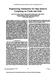


![Extreme Data-Intensive Computing - salsahpc [PDF]](https://m.moam.info/img/260x300/extreme-data-intensive-computing-salsahpc-pdf_64a65720098a9e9f698b45b9.jpg)
