Feb 6, 2015 - 7.1 Introduction. ZigBee transceivers are being encouraged in this last decade for ultra-low power, low-cost low-data-rate wireless applications.
7 Design of an Energy-Efficient ZigBee Transceiver Antonio Ginés, Rafaella Fiorelli, Alberto Villegas, Ricardo Doldán, Manuel Barragán, Diego Vázquez, Adoración Rueda, and Eduardo Peralías CONTENTS 7.1 Introduction................................................................................................. 171 7.2 The ZigBee Standard.................................................................................. 172 7.2.1 ZigBee Transceiver Architectures................................................ 172 7.2.2 Transceiver Requirements for ZigBee.......................................... 173 7.3 Proposed Receiver Synthesis..................................................................... 173 7.3.1 RX: Architecture Selection............................................................ 173 7.3.2 RX: Building Blocks Specifications............................................... 175 7.3.3 RX: Gain, Noise and Linearity Distribution Procedure............ 178 7.3.4 RX: Optimization and Verification............................................... 183 7.4 Proposed Transmitter Synthesis............................................................... 185 7.4.1 TX: Architecture Selection............................................................. 185 7.4.2 TX: Building Blocks Specifications............................................... 186 7.4.3 TX: Gain, Noise, Linearity, Power Distribution Procedure and Other Specifications................................................................ 190 7.4.4 TX: Power Amplifier Optimization.............................................. 194 7.5 Example of Integrated Transceiver........................................................... 195 7.6 Conclusion................................................................................................... 198 Acknowledgment................................................................................................. 199 References.............................................................................................................. 201
7.1 Introduction ZigBee transceivers are being encouraged in this last decade for ultra-low power, low-cost low-data-rate wireless applications. In most cases, these devices should be able to operate from a battery with a life time of years. Typical applications for this standard include diverse areas in the industry or home automation. Of relevant interest, we can highlight its specific use to create and to control the smart grids which distribute the utilities 171
K24255_C007.indd 171
02-06-2015 20:42:17
172
Mixed-Signal Circuits
(as electricity, gas, and water). In order to achieve the power targets, it is critical not only to have low power consumption during transmission and reception, but also to be able to have a fast wake up time, so that the devices can be most of the time in sleep mode. This chapter tries to summarize our experience in the development of the analog front-end part of 2.4 GHz ZigBee transceivers with the main objective of optimizing power consumption during normal operation in both reception (described in Section 7.3) and transmission modes (at Section 7.4). Other interesting design aspects, such as optimizing the transceiver protocol, the design of the digital subsystems, or managing the sleep modes, have not been included due to space limitation. To gather together the presented design ideas, the chapter concludes in Section 7.5 with an example of an integrated complementary metal-oxide semiconductor (CMOS) transceiver analog front-end. The competitive experimental performances for this integration endorse the employed design flow, procedures, and analysis.
7.2 The ZigBee Standard ZigBee® is a standard developed by the ZigBee Alliance (www.zigbee.org), built in 2002, that defines a communication protocol for short-range wireless networking mainly covering applications where low-data-rate, low cost, and long battery life are required. ZigBee is compliant in its physical layer and medium access control protocols with the IEEE 802.15.4 standard [1]. Operation frequency bands are 868 MHz, 915 MHz, and 2.4 GHz with a maximum data rate of 250 kb/s. ZigBee uses spreading methods to improve the receiver sensitivity level, to increase the jamming/interference resistance, and to reduce the effect of the multipath. The spreading method used in the 2.4 GHz-band is the direct sequence spread spectrum (DSSS). Data bit streams going at 250 kbps, after the spreading, are transformed in pseudo random sequences of bits, named chips, at a rate of 2 Mbps. Number of channels in this band are 16 (of 5 MHz-wide each one) and distributed between frequencies of 2402.5 and 2482.5 MHz. Sensitivity of the receiver in each channel has been specified from −85 to −20 dBm input power for detection error rates less than 1% with 208-bit information packets in a range up to 100 m. The transmitter output level must reach at least −3 dBm with a variable adjustment of 30 dB. 7.2.1 ZigBee Transceiver Architectures The choice of the receiver and transmitter architectures in a ZigBee transceiver strongly determines the performance of the whole system, especially concerning power consumption. Architecture selection has been widely
K24255_C007.indd 172
02-06-2015 20:42:17
Design of an Energy-Efficient ZigBee Transceiver
173
analyzed in many recent works—a good survey of them appears in [2]. The work in this chapter uses the one shown in Figure 7.1, which is the widest accepted in the state-of-the-art of 2.4 GHz transceivers. It comprises a low-IF chain with complex filters [3] for the receiver (RX) and a Direct-Up Conversion architecture [4] for the transmitter (TX). More details of selected architectures are given in Sections 7.3 and 7.4, respectively. Both receiver and transmitter share a PLL frequency synthesizer as local oscillator (LO), which is based on a simple integer-N scheme with the VCO running at double frequency of the RF band (~5 GHz) [5]. The clock frequency of the receiver chain ( f LOD) has an offset from the RF central frequency ( f RF) of the reception chan- Q1 nel, in an amount equal to the desired low-intermediate frequency ( f IF) in baseband (BB) for the down-converted signal. In transmitter chain, the clock frequency ( f LOU) coincides with f RF frequency. 7.2.2 Transceiver Requirements for ZigBee The electrical characteristics for the receiver and transmitter—noise figure (NF), input level for the third order intermodulation product (IIP3), output compression point (OP1dB), image rejection ratio (IRR), and error vector magnitude (EVM), are not specified in the ZigBee standard, so they have to be obtained from system specifications, which are in physical layer: the data rate, the modulation and spreading types, the receiver sensitivity and jamming resistance, and the mask of output power spectral density. In this chapter, only a summary with the most representative specifications are given (see Table 7.1), but the interested reader can find a detailed procedure to obtain them in [6].
7.3 Proposed Receiver Synthesis 7.3.1 RX: Architecture Selection The first step in the receiver synthesis is the choice of the optimum architecture for a fully integrated low-power design. The decision was restricted between the direct conversion and the low-IF topologies, since the heterodyne receiver [4] would generally require external components and it uses two different frequency down-conversion steps with the consequent area, cost, and power consumption penalties. Among the two candidates, and taking into account that the image rejection specifications in the ZigBee standard are not very restrictive (image rejection ratio IRR > 30 dB is safe enough), the low-IF approach was finally selected because it relaxes the DC offset and flicker noise in the receiver BB section. Figure 7.1 shows the details of the resulting low-IF receiver (RX). A fully differential implementation is considered to improve noise immunity and
K24255_C007.indd 173
02-06-2015 20:42:17
K24255_C007.indd 174
RX/TX
0 90
Transmitter (TX)
PA
2 × fLO
÷2 fLOU = fRF
sin(ω LOUt)
Quadrature up-converter
cos(ω LOUt)
fLOD = fRF – fIF
Channel selection and image rejection
Complex filter
sin(ω LODt)
Quadrature Up-converter
cos(ω LODt)
IQ mixers
FIGURE 7.1 Proposed ZigBee architecture: Low-IF receiver and direct conversion transmitter.
Band filter
fckREF
PLL (LO)
LNA
Receiver (RX)
BB filter
BB filter
VGA
VGA
DAC
DAC
ADC
ADC
QinBB
Digital baseband generator
IinBB
QoutBB
DSP
IoutBB
174 Mixed-Signal Circuits
02-06-2015 20:42:18
Design of an Energy-Efficient ZigBee Transceiver
175
common-mode rejection. The RF signal is amplified by the front-end lownoise amplifier (LNA) and down-converted to the intermediate frequency (IF) by two mixers in quadrature (IQ-mixers). Channel selection and image rejection are performed by an active complex filter. Finally, the IF in-phase and quadrature (I/Q) signals are passed through the variable-gain amplifiers (VGAs) to adequate their amplitude to the input ranges of the back-end analog-to-digital converters (ADCs). The choice of the intermediate frequency requires a trade-off between power consumption and noise. A widely accepted compromise is to use an IF frequency equal (or slightly larger) than the signal bandwidth (2 MHz in ZigBee). Considering extra safety margin for relaxing the DC-coupling networks between stages and flicker noise requirements, a 2.5 MHz IF was finally set as a good compromise. This selection has the additional advantage of simplifying the PLL frequency divider establishing an integer relationship between the input clock reference ( fckREF = 2.5 MHz) and the synthesizer output frequencies, f LOU = N ⋅ fckREF, f LOD = (N − 1) ⋅ fckREF. 7.3.2 RX: Building Blocks Specifications When compared to the transmitter channel, the task of determining the building block specifications in the receiver path is especially complex since the input signal power level will cover several decades—in the transmitter counterpart, the difficulty is not found in the size of design space, but in the close coupling between up-converter and PA specifications which require a co-design at circuit level, as will be shown in Section 7.4. In the ZigBee standard, the input power specification must be verified within a nominal power input range from −85 dBm to −20 dBm. In practice, extra safety margins at the upper level should be also allocated for robustness against possible interferences. A maximum power level of Pin = −16 dBm could be a good choice, this meaning a sensitivity range of 78 dB for the complete channel. Once the architecture has been selected, we have to determine the circuitlevel realization and specifications for the different building blocks. This implies finding noise and distortion error budget distribution among the receiver stages to satisfy the target performance, while minimizing power consumption. The key specifications include the average power consumption of each building block (PAVG,i), input-referred noise voltage or noise figure (NFi), input-referred intermodulation products of third and second orders (IIP3,i, IIP2,i), power gains (Gi), and the internal power levels (Pi) at the input of the different stages in the receiver queue (STGi), where the subindex i ∈ [1, NSTG] specifies the order of a particular block in the chain from the antenna, {STG1 = Band Filter, STG2 = LNA, . . . , STGNSTG = ADC} in the implementation of Figure 7.1, and P1 ≡ Pin is the input power to the receiver. Due to its difficulty, this task has been traditionally addressed by a high qualified engineer, the so-called RF cook, who often performs a manual
K24255_C007.indd 175
02-06-2015 20:42:18
176
Mixed-Signal Circuits
channel sizing based on his previous expertise and knowledge of technology limits from different integrations and assisted by more or less complex distributing tools (as ADSTM from Agilent Technologies). As shown in the RF receiver model of Figure 7.2, critical aspects—such as distribution of power consumption per stage (PAVG,i),, number (NG) of programmable gain modes to satisfy the target requirements at all internal input levels (Pi), input signal power thresholds between modes (Pth,j), and specific gain distribution set {Gi,k}j, where j ∈ [1, NG] specifies a particular gain mode—could lead to a tedious iterative process which eventually conduce to no solution, especially when complex trade-offs or target specifications close to the technological limits are present. Even if a solution is found, manual sizing usually leads to nonoptimum designs in terms of power consumption. In [7], a guided synthesis procedure for RF receiver channels was proposed considering semi-analytical expressions. The main limitation of this approach is the lack of models that incorporate gain as a design parameter. Hence, it needs some manual adjustment when different gain-programmability modes are defined in the power range of input signal. As alternative to overcome these drawbacks, we have introduced a systematic procedure for automatic synthesis of RF receivers with emphasis in power optimization. Following a top-down bottom-up design flow, the procedure provides an energy efficient distribution of gain and power between stages, and hence, an optimum allocation of noise and distortion error budget. As will be seen in Section 7.3.3, the proposed design flow is suitable for most of the RF chains and other specific transistor-level realizations of the building blocks. In Section 7.3.4, it is applied for power optimization of the low-IF receiver in the ZigBee transceiver of Figure 7.1 as demonstrator. Figure 7.3 shows the simplified schematics of the main building blocks in this case of study. The front-end LNA (Figure 7.3a) uses a differential common source stage with inductive degeneration [8]. Both IQ-mixers share the same active implementation in Figure 7.3b [9] inspired on a Gilbert multiplier, but
Gain programmability
(G1,r) Pin = P1 j
G3,3 G3,2
G1,2 G2,1
G1,1 STG1 rj
P2
STG2
PAVG,1
G3,1 P3
STG3
PAVG,2 K j
G1,2G1,2G3,3
P4
G1,1G2,1G3,2 G1,1G2,1G3,1
{G3,K}
j=1 G3
j=2
G3,3
j=3
G3,2
G3,1
PAVG,3 G1
Gain mode selection
Total gain in different gain modes
G(j)
(P(i+1) = Gi,k . Pi
Total power (PAVG) = PAVG,1 + PAVG,2 + PAVG,3
G1,1
G1,2 Pth, 1
Pth,2
Pin
FIGURE 7.2 Conceptual example of a RF receiver with NG = 3 different gain modes, j ∈ [1, 3].
K24255_C007.indd 176
02-06-2015 20:42:18
K24255_C007.indd 177
2
2
Preamp
Preamp
Cext
Lg
Rbias
Cd2
2
2
M1
M3
gmB –gmA
−
VFinQ
+
2nd-order section 1
gmA
Vin
Ld VDD Cd2
Cext
gm1 C1
2
–gmD VoutQ
–gm2
–gm4 gm3 C2
Vout
(Single-ended schematic)
2nd-order section 2
gmD –gmC
2
V−in
VoutI
Vp1
V+out
Lg Cblock
Rbias
Cd1
2nd-order section 2
M2
M4
gmC –gmB
2 × Ls
2nd-order section 1
VDD
Cd1
Ld
(d)
(b)
Co
Cz
F5Ib
M5
STG core
Voutp
Vinn
Vinp
LO
VB +VRF/2
−
+
C1
Vinp,2
M1
BiasP
Vinn,2
M3 BiasN
cmi
+ −
Igc
+
CMOS buffer
M7
RL V+out
Vdd
STG1
M8
M9
V1
Rz
Io1
Ro
Digital gain control
+ −
−
M4 FNIb
M2
cmi VREF
CMFFC
XL O
M6 Co
Voutn
Ro
VB – VRF/2
(FN + F3)Ib
2
(Vbp,Vbn)
Voutp Voutn
Io2
M10
M6 M5
V−out
STG2
Vbn
2RS
Vbp
−
+
RL
Vdd
FIGURE 7.3 Simplified schematic of the main building blocks in the receiver chain: (a) LNA, (b) IQ-mixers, (c) Complex Filter, and (d) VGA.
−
VinQ
+
VinQ
VinI
(c)
V+in
Cblock
Vp1
V−out
(a)
Design of an Energy-Efficient ZigBee Transceiver 177
02-06-2015 20:42:19
178
Mixed-Signal Circuits
the differential pair associated with the local oscillator (LO) is substituted by a CMOS digital buffer [10]. An impedance adaptation network between LNA and IQ-mixers has been used for their coupling. The channel filter in Figure 7.3c [11] comprises a pre-amplifier followed by an 8th-order bandpass complex filter core (two second-order bandpass Gm-C sections in cascade). The preamplifier sets the common-mode of all used transconductors in the filter. The last key block in the receiver chain is the VGA in Figure 7.3d which provides signal conditioning for the ADCs. A multistage VGA architecture is considered. Each stage core is formed by a gain boosted amplifier with resistive degeneration, since this topology presents an optimum trade-off between nonlinear response and power consumption for ZigBee receivers [12]. The specific number of stages in the VGA has also been included in the optimization process. In the integrated example (see Section 7.5), two stages were implemented. 7.3.3 RX: Gain, Noise and Linearity Distribution Procedure This subsection introduces the fundamental concepts of the proposed design flow. The synthesis is formulated as an optimization problem with multiple constrains, generally described in the form, find x = {N G , {Pth , j } j =1…NG −1 , {Gi , k j } j =1…NG , {PAVG , i }i =1…NSTG } � NSTG
which minimizes : PAVG ( x) = �
∑P
AVG , i
i =1
(7.1)
constrained by: NF(Pin ) ≤ NF spec (Pin ); IIP3 (Pin ) ≥ IIP3spec (Pin );
IIP2 (Pin ) ≥ IIP2spec (Pin )
Taking into account the target specifications of the receiver chain (see Table 7.1)—that is, the total NFspec and intermodulation products (IIP3spec , IIP2spec ) as function of the input signal power (Pin), the objective of the synthesis procedure is to find the number of gain modes (NG) and their distribution along the input power range (Pth,j), the specific gain distribution set {Gi,k}j in each mode and the power consumption per stage PAVG,i, which minimize the total power consumption, PAVG = ∑PAVG,i, once all targets are satisfied. Considering this formulation of the problem, that can be obviously generalized with other target constrains, a top-down bottom-up design flow has been developed for automatic synthesis of the receiver channel. Its flow diagram is illustrated in Figure 7.4. Starting from specifications, the topology generator (see label step1 in the figure) defines which stages in the receiver queue have the possibility of gain programmability and determines the number of gain levels (Li) for these blocks. This phase in the design flow requires a close interaction with block designers to assure that the inclusion of programmability does not affect the block performance. In the example
K24255_C007.indd 178
02-06-2015 20:42:19
179
Design of an Energy-Efficient ZigBee Transceiver
TABLE 7.1 Summary of the Transceiver Electrical Specifications and Constraints Receiver Specification Input power range Noise figure IIP3 IIP2 Spurious free dynamic range Channel selectivity requirements
Value (−85, −20) dBm −35 + ( Pin + 85) dBm >−10 dBm >−20 + (Pin + 85) dBm >5 dBm >32 dBm −60 dBm adjacent channels (±5 MHz) alternate channels (±10 MHz)
for 1000 chips at −3 dBm output power
of Figure 7.2, programmability was included in first and third stages (STG1, STG3) with L1 = 2 and L3 = 3. The topology generator could also incorporate critical design parameters (DPi) in some specific building blocks, when there exist complex trade-offs between specifications. As an example, the DPi could be the biasing conditions (gm/ID) of the main transducer transistors (these transistors determine in each circuit implementation the main tradeoff between noise and distortion for a given power consumption, PAVG,i). Taking into account the outputs of the topology generator, the synthesis procedure performs an optimization loop to minimize power consumption while achieving specifications in each design (step 2). In our case, the whole synthesis loop is supported by MATLABTM and the external optimization tool Fridge [13], which is the engine that processes performance results and generates new iterations seeds following a simulated annealing algorithm. In each iteration, the design variables (step 3) are reduced to the average power consumption (PAVG,i) and the specific values of the gain in each stage (including programmability). In the conceptual example of Figure 7.2, the set of gains were {G1,1, G1,2, G2,1, G3,1, G3,2, and G3,3}. From these values, and taking into account technology look-up tables (LUTs) which characterize the performance of the building blocks at transistor levels, the high-level parameters of each stage are derived in step 4 as a function of Pi. In this step, the parameter Pi should be understood just as an
K24255_C007.indd 179
02-06-2015 20:42:19
K24255_C007.indd 180
New design {Gi,k}, PAVG,i
Topologies
Step4
End? Yes
Determination of gain modes: j, Pth,j, {Gi,k}j
Step7
Performance evaluation NF (Pin) IIP3 (Pin), IIP2 (Pin)
Step6
Step5 Specific input signal power levels: Pi
STGi parameters: NFi (Pi) IIP3,i(Pi), IIP2,i(Pi)
Optimization summary
No
FIGURE 7.4 Basic flow diagram of the receiver synthesis procedure.
FridgeTM
Step2 Optimization: min(PAVG)
Step3
All combinations: {Gi,k}
Design-variables space reduction
Initial design {Gi,k}0, PAVG,i0
MATLABTM
Step1 Topology generator gain programmability, Li , DPi
Receiver specifications NF spec(Pin), IIP3spec(Pin), IIP2spec(Pin)
End
LLS
Saturation model
Transistor-level lookup tables
{Gi,k}, PAVG,i, DPi
Low-level specifications: HD1(Pi), IM3(Pi), Gi(Pi)
180 Mixed-Signal Circuits
02-06-2015 20:42:20
181
Design of an Energy-Efficient ZigBee Transceiver
independent variable which defines the mathematical relationship between the high-level parameters and the signal power at the input of each stage. The specific distribution of signal power along the channel queue will be later evaluated at step 5, as described next in detail. In our ZigBee case, the effective noise figure NFi and intermodulation products (IIP3,i and IIP2,i) are inferred from the low-level specifications tabulated in the LUTs. Depending on the building block, these LUTs could incorporate different specifications, such as: the amplitude of the first harmonic (HD1), the effective gain (Gi, from which the 1 dB compression point can be extracted) or the third-order intermodulation products IM3, all of them evaluated as a function of Pi based on transistor-level simulations with one-tone and/or twotone input stimuli. As an example of the information capture in the LUTs, Figure 7.5 shows the transistor-level simulations of a two-tone test for an implementation of the IQ-mixers in Figure 7.3b in a 1.2 V 90 nm CMOS process. Details on the amplitude of one of the tones HD1 and the corresponding intermodulation product IM3 for two possible gain values are depicted. It is worth noticing that in order to reduce the design effort and characterization time during the LUT generation, the determination of the high-level parameters in step 4 could be supported by analytical expressions which allow expanding the covered design space as function of the power consumption on each block (PAVG,i). In our ZigBee case, the information in the LUT has been processed by means of two analytical expressions, denoted by IQ mixer transistor-level simulations (two-tone test)
0 –10 –20 –30 –40 –50 –60
HD1(dB): High gain mode HD1(dB): Low gain mode IM3(dB): High gain mode IM3(dB): Low gain mode
–70 –80
–80
–70
–60
–50
–40
–30
–20
–10
Pi (dBm) FIGURE 7.5 Transistor-level simulations of HD1 and IM3 versus input signal power of an implementation of the IQ-mixers in Figure 7.3b in a 1.2 V 90 nm CMOS process.
K24255_C007.indd 181
02-06-2015 20:42:20
182
Mixed-Signal Circuits
NFi = fi(Pi, PAVG,i) and IIPx,i = gx,i(Pi, PAVG,i, Gi,k) which depends on the specific building block realization (similar expressions could be derived for other additional targets). The agreement between these analytical predictions and transistor-level simulations for different requirements in term of average power consumption of the block (PAVG,i) and gain selection (Gi) were verified by multiple designs in each building block. Although the detailed descriptions of these expressions are out of the scope of this chapter, we would like to highlight that they capture the natural design knowledge in terms of noise and distortion for a given design biasing conditions; these are: (a) the noise or equivalently NFi can be reduced incrementing power consumption, and (b) given an input signal power Pi, the input referred intermodulation products (IIP3,i and IIP2,i) have an inverse relationship with gain since nonlinearities increase with the signal level. In step 5, the amplitude signal levels at the different stages are evaluated for the specified power input range at the antenna (from −85 to −16 dBm in our ZigBee demonstrator), and for all the possible gains combinations. In the example of Figure 7.2, the set of gains has six possibilities, given by: {G1,1G2,1G3,1, G1,2G2,1G3,1, G1,1G2,1G3,2, G1,2G2,1G3,2, G1,1G2,1G3,3 and G1,2G2,1G3,3}. For each gain distribution, the specifications of the receiver channel are evaluated—in step6—as a function of the input power: f(Pi, PAVG,i), g3(Pi, PAVG,i, Gi) and g2(Pi, PAVG,i, Gi). This evaluation is based on the classical Frii’s formula for the determination of the NF in a RF channel with m stages in cascade, given by NF = 1 + (N F1 − 1) +
(NF2 − 1) (NF3 − 1) (NFm − 1) + +�+ G1 G1 ⋅ G2 G1 ⋅ G2 � G( m −1)
(7.2)
and the equivalent expression for the inter-modulation products, 1
2 aIIP 3
=
1 2 aIIP 3 ,1
+
A12 2 aIIP 3 ,2
+
A12 ⋅ A22 � A(2m −1) A12 ⋅ A22 + � + 2 2 aIIP aIIP 3,3 3 ,m
(7.3)
A ⋅ A2 � A( m −1) 1 1 A1 A ⋅ A2 = + + 1 +�+ 1 aIIP2 aIIP2,1 aIIP2,2 aIIP2,3 aIIP2,m
(7.4)
where aIIPx,i stands for the input referred to as rms amplitude (in Volts) of the intermodulation products, and Ai is the linear voltage gain of the ith block. In these traditional formulas, two aspects were particularized to take into account that: (1) impedance matching is not necessary, and (2) the signal level excursions at the input of each block cannot be arbitrarily defined, since the available voltage range is limited depending on the circuit-level realization. According to the first aspect, the input referred to as voltage noise of the BB section has been translated to an effective NF which considers degradation in the signal-to-noise ratio. Regarding the second consideration, a soft
K24255_C007.indd 182
02-06-2015 20:42:21
Design of an Energy-Efficient ZigBee Transceiver
183
saturation model has been included in such a way that situations with excessive gains result penalized in the optimization process, and therefore, it leads to noncompetitive designs in terms of power and performance (discarded by the search engine). The key idea of this soft saturation model is to introduce a degradation of the NF and intermodulation products when the amplitude signal levels exceed a safety region boundary in each design. The final step in each iteration (step 7) consists of determining the optimum number (NG) of gain distributions modes and power thresholds Pth,j between gain modes. To carry out this selection, the channel performance evaluated in step 6 is used for all the possible gain combinations to determine the gain subset {Gi,k}j which provides the best performance for each input power level (Pin). In the example of Figure 7.2, the six gain possibilities are finally reduced following this criterion to just three cases (NG = 3): {G1,1G2,1G3,1, G1,1G2,1G3,2 and G1,2G2,1G3,3}. The optimization of each topology finishes when all specifications are met and minimum power consumption is found by the optimization tool. This process usually takes less than half an hour per topology. If no solution is found for a specific case, maximum number of iterations is defined and the incidence will be back-annotated in the final optimization summary. 7.3.4 RX: Optimization and Verification In this section, the final optimization results for the ZigBee receiver design is presented, as well as the corresponding verification simulations. These results have been carried out using the synthesis procedure presented in previous sections with multiple iterations to refine the topology and critical design parameter (DPi) constrains captured by the LUTs. The convergence of the whole process was quite fast, requiring just three iterations at the top level (including the refinement of LUTs) to achieve the optimum topology with minimum power consumption (17 mW for the receiver channel, excluding the PLL 6.9 mW, and mixer drivers 7.4 mW). Table 7.2 shows a summary of the derived specifications with details on the gain programmability for each building block. The optimization procedure introduced programmability in all stages excluding the front-end LNA—the inclusion of gain programmability in the LNA was also considered in the optimization problem, but these solutions resulted not efficient in terms of power consumption, and therefore, they were automatically discarded in the process. In Table 7.3, the optimum gain distribution as function of the input power (Pin) is presented. In total, 13 different gain modes were selected for the best performance (NG = 13). Considering the above optimum distribution of gains, Figure 7.6 shows the overall performance results based on MATLAB simulations. They include the total NF and third intermodulation products (IIP3 and IIP2) as a function of input power. In each case, limits imposed by the ZigBee standard (see Table 7.1) have been highlighted, clearly showing that all specifications are satisfied.
K24255_C007.indd 183
02-06-2015 20:42:21
184
Mixed-Signal Circuits
TABLE 7.2 Main Optimization Results for the Specifications of the Main Building Blocks in the Channel Receiver with Details on the Gain Programmability Modes Gain Programmability per Building Block Receiver Block LNA
Mixer
Channel Complex Filter
PGA Stage
ADC
Specification Power gain (dB) Power (mW) NF (dB) IIP3 (dBm) IIP2 (dBm) Conversion gain (dB) Power (mW) SSB NF (dB) IIP3 (dBm) IIP2 (dBm) Voltage gain (dB) Power (mW) Input noise (V/√Hz) IIP3 (dBV) IIP2 (dBV) Voltage gain (dB) Power (mW) Input noise (V/√Hz) IIP3 (dBV) IIP2 (dBV) Power (mW) Full scale (V) Resolution (effective bits)
1
2
3
4
5
6 1.44 5 −7 15 6 2 × 4.92 18 3 25 0
15 18 1 20 12 3.60
100
25
−3 12 0
−8 7 6
36 10 27 2 × 0.2 1 6
12 4 × 0.56 33 26 10 3 22 17
18
24
18
13
−4 12
−10 7
The agreement of the specifications assignment with the standard has been alternatively validated using Agilent advanced design system (ADSTM) simulator. Figure 7.7 shows the simulation setup for the ZigBee receiver. In this environment, behavioral simulations include relevant nonideal effects such as channel noise, distortion, phase noise, and I/Q imbalance. The performance of the receiver was exhaustively characterized in terms of error rate. As an example, Figure 7.8 shows the sensitivity simulation by varying the input power level. For the required chip error rate (CER) of 6.89% (i.e., 1% packet error rate PER), the input power of the receiver is about −88 dBm with a system NF of 21 dB. This simulation not only includes the noise effects but also the distortion in the receiver blocks and phase noise in the LO. As it can be observed, the chip error rate is below 6.89% in the whole standard input range (from −85 to −20 dBm), corroborating that the chosen
K24255_C007.indd 184
02-06-2015 20:42:21
185
Design of an Energy-Efficient ZigBee Transceiver
TABLE 7.3 Optimization Results for the Gain Distribution among the Receiver Chain Input Range (dBm)
Voltage Gain (dB)
Gain Modes
From
To
Band Filter
LNA
Mixer
Channel Filter
1 2 3 4 5 6 7 8 9 10 11 12 13
−90 −84 −78 −72 −66 −63 −57 −51 −45 −39 −33 −27 −22
−85 −79 −73 −67 −64 −58 −52 −46 −40 −34 −28 −22 −16
−3 −3 −3 −3 −3 −3 −3 −3 −3 −3 −3 −3 −3
6 6 6 6 6 6 6 6 6 6 6 6 6
15 15 15 15 6 6 6 6 6 6 6 6 6
12 12 12 12 12 12 12 12 12 12 12 0 0
VGA STG 1 24 24 24 24 24 18 18 12 6 6 0 6 0
VGA STG 2 24 18 12 6 12 12 6 6 6 0 0 0 0
RX Gain (dB) 78 72 66 60 57 51 45 39 33 27 21 15 9
distribution of specifications among receiver building blocks meets the standard requirements. Figures 7.9 and 7.10 show some details of the eye diagram and the I/Q constellation in two extreme input power level. Some effects, as the phase noise and amplitude saturation over the receiver output signals, can be appreciated clearly in these figures.
7.4 Proposed Transmitter Synthesis 7.4.1 TX: Architecture Selection The low-power and completely-integrated transmitter required for the desired application only admits certain types of architectures. The one chosen in this implementation is the direct up-conversion transmitter (DUCT) of Figure 7.1, which, despite its known drawbacks due to high dc-offset and flicker noise values [2], is a good choice because of the reasonable transmitter input levels. To make this architecture effectively feasible, some efforts in reducing offset and mismatch should be done since they cause LO feedthrough, which overlaps with the modulated carrier at frequency f RF. This way it is possible that the DUCT correctly achieves EVM ZigBee specifications (EVM ≤ 35% at ZigBee 2.4 GHz), as shown afterward.
K24255_C007.indd 185
02-06-2015 20:42:21
186
Mixed-Signal Circuits
(a) 90
Noise figure (dB)
80
Maximum allowable NF for IEEE 802.15.4 Overall system NF from receiver blocks
70 60
NFspec(Pin)
50 40 30 20 10 –90
–80
–70
(b) –5
–60 –50 –40 Input signal power (dBm)
–30
–20
–10
–10 IIP3 (dBm)
–15 –20
IIP3spec(Pin)
–25 –30
Maximum allowable IIP3 for IEEE 802.15.4 Overall system IIP3 from receiver blocks
–35 –40 –90
–80
–70
(c) 30
–60 –50 –40 Input power range (dBm)
–30
–10
–20
–20 IIP2 (dBm)
–10 0
IIP2spec(Pin)
–10
Maximum allowable IIP2 for IEEE 802.15.4 Overall system IIP2 from receiver blocks
–20 –30 –90
–80
–70
–60 –50 –40 Input power range (dBm)
–30
–20
–10
FIGURE 7.6 Optimization results for the overall receiver specifications: (a) NF; (b) IIP3; (c) IIP2.
7.4.2 TX: Building Blocks Specifications Both the ZigBee physical layer and the transmitter architecture, in this case the DUCT of Figure 7.1, determine the specifications of its building blocks. For the DAC, its minimum number of conversion bits is derived from the
K24255_C007.indd 186
02-06-2015 20:42:22
K24255_C007.indd 187
Signal source
Interferers
Transmitter
AWGN CHANNEL LNA – IIP3 – NF – Gain – Rin
VGA
– Filter order – Cutoff freq. – Gain – IIP3 – Noise – IRR – fIF and BW
Channel filter
– IIP3 – NF – Conversion gain – RF-LO isolation – I/Q imbalance – LO Phase noise
Quadrature down-converter
FIGURE 7.7 Simulation scheme for the ZigBee receiver in Agilent advanced design system (ADS).
Data stream
Receiver
– IIP3 – NF – Gain
– Bits resolution – Sampling CLK
ADC
Demodulator and data decoding
BER constellation
Design of an Energy-Efficient ZigBee Transceiver 187
02-06-2015 20:42:23
Mixed-Signal Circuits
Chip error rate Gain
100
10 6.89% (IEEE 802.15.4)
0 –100
–90
–80
–70
–60 –50 Input power (dBm)
–40
–30
50
Gain (dB)
Chip error rate (%)
188
0 –20
FIGURE 7.8 System simulation results in the receive path: sensitivity performance.
ZigBee SNR as follows. As the absolute limits of spurious outside the band must be below 30 dB [1] and each bit of resolution improves 6.02 dB, then the DAC should have, at least, 5 bits. Also, to improve the SNR, the signal is oversampled eight times the chip rate, that is, fCLK,DAC = 16 MHz [6]. The BB filter is employed to reduce the power of the DAC output images. Its corner frequency can be as low as the bandwidth of ZigBee signal (~1.5 MHz), and the use of DAC oversampling relaxes its design up to very low-order IoutBB (LSB)
32
16
16
Pin = –20 dBm RX gain = 21 dB
0
Pin = –20 dBm RX gain = 21 dB
0
–16
–16
–32 32
–32 32
Pin = –80 dBm RX gain = 72 dB
16
16
0
0
–16
–16
–32
QoutBB (LSB)
32
0
0.2
0.4 0.6 Time (μs)
0.8
1
–32
Pin = –80 dBm RX gain = 72 dB
0
0.2
0.4 0.6 Time (μs)
0.8
1
FIGURE 7.9 System simulation results in the receive path: eye diagram for two different input power levels.
K24255_C007.indd 188
02-06-2015 20:42:24
189
32
32
16
16 QoutBB (LSB)
QoutBB (LSB)
Design of an Energy-Efficient ZigBee Transceiver
Pin = –20 dBm RX gain = 21 dB EVMrms = 11.26%
0
EVMrms = 40.77%
0
–16
–16
–32 –32
Pin = –80 dBm RX gain = 72 dB
–16
0
IoutBB (LSB)
16
32
–32 –32
–16
16 0 IoutBB (LSB)
32
FIGURE 7.10 System simulation results in the receive path: I/Q constellation for two input power levels.
type (~second-order), resulting in EVM less than 5% [14]. The variation in the transmitter’s output power can be completely gathered in the BB filter, by means of a variable gain (e.g., having an attenuation of up to 30 dB in steps of 1 dB) to relax the amplitude requirements of following blocks. For the DAC and the BB filter, the I/Q mismatch should be reduced, in order to avoid cross-talk between the two data streams modulated on the quadrature signals of the carrier, as it would create an undesired sideband signal at the output, placed symmetrically respect to f RF. Those mismatches are described in terms of rejection of the unwanted single-sideband (SSB). Considering an SSB rejection of 30 dB [1], the I/Q mismatch contribution in EVM should be below 3.2%. The up-conversion mixer should have a double-balanced structure so as to achieve high isolation between LO and RF ports. The typical carrier leakage specifications in this block achieve −30 dBc, resulting in an EVM contribution of less than 3.2%. Also, mixer nonlinearities generate in-band spurs. For ZigBee, a 30 dB attenuation of these spurs respect to the output signal means a reasonable EVM of 3.2%. Moreover, mixer linearity requirements are derived as follows: the OP1dB for the DUCT is generally fixed to at 0 dBm, above the nominal Pout (=−3 dBm); hence, in a first approximation, 10 dB can be considered the minimum mixer OIP3 [4]. Finally mixer’s conversion gain is adjusted to achieve the desired input amplitude of the PA, as it will be explained in Section 7.4.3. The final block of the chain, the power amplifier (PA), must provide a maximum Pout of, at least, 0 dBm for a standard output impedance as 50 Ω (linearity constraints are the same as in the mixer). As ZigBee applications have to be low power consumption, PA efficiency is a concern. To achieve the required maximum output power with the best efficiency, the election of the
K24255_C007.indd 189
02-06-2015 20:42:24
190
Mixed-Signal Circuits
CGmixer+INW = 5 dB ioMIX+ VIinBB VQinBB
Active Up-Conversion Mixer
INW
VinPA+
+ RL
PA ioMIX–
cos(ωLOUt)
GPA = 10 dB
VinPA–
Vo –
sin(ωLOUt)
Vin,DC
VDD
Rb
Vin,DC Rb
Vin,PA+
Vin,PA– PA
+ Vo –
FIGURE 7.11 Scheme of the transmitter blocks and PA differential topology (detail).
PA sizing as well as its bias and input signal amplitude is made carefully [15]. To transform the output amplitude of the mixer into the required PA input signal amplitude, without high losses, an interface network INW is needed between both blocks, as seen in Figure 7.11. The DUCT PA carrier frequency f RF is equal to that of the LO, hence the former might represent an interference in the LO, that is, LO pulling [4]. It is worse, if the system integrates the voltage-controlled oscillator (VCO) and the PA on the same chip. To reduce this effect, it is desirable to use a VCO working with twice the channel frequency ( f VCO = 2f RF). This approximation has been implemented in our transceiver. To evaluate the total DUCT EVM, it is assumed that the EVM contributors above mentioned are uncorrelated, hence the total DUCT EVM is the rootmean square (RMS) sum of the individual components [14], resulting in a total EVM of 7.5% for the transmitter chain up to the PA. Compared to 35% from ZigBee requirements, this leaves a wide safe margin for the PA inherent nonlinearity. 7.4.3 �TX: Gain, Noise, Linearity, Power Distribution Procedure and Other Specifications After the presentation of the main specifications of the DUCT blocks, the final distribution of power consumption budget, gain, and linearity are
K24255_C007.indd 190
02-06-2015 20:42:25
Design of an Energy-Efficient ZigBee Transceiver
191
discussed here. When compared to the receiver counterpart in Section 7.3.3, the design space is now more reduced in terms of input range and channel selectivity. However, its implementation presents multiple interrelations between blocks at circuit level, especially at the interface network INW between up-converter mixer and PA, making necessary the developing of a different optimization approach. To do so, we use a combination of a bottomup methodology together with a top-down methodology which incorporates the simultaneous co-design between critical blocks at transistor level. Initially, the distribution of blocks specifications is chosen by considering both state-of-the-art designs and our previous experience, and then optimization procedures are followed in each block, for example, the PA design is done following an optimization procedure to obtain the most efficient of the Class-AB architecture used, as discussed in Section 7.4.4. Next, high-level simulations are carried out in MATLAB and ADS software to distribute optimally the budget of power consumption, gain and linearity, and to check the achievement of specifications during all the design procedure. The reduction of transmitter power consumption is a great concern in the whole ZigBee DUCT design. Its reduction strongly depends on the PA output power, Pout, on the appropriate distribution of gain and IIP3 between DUCT blocks, and on the correct power transfer between the mixer and the PA. There is an inherent trade-off between power and the other characteristics that have to be considered, since reducing power consumption degrade the linearity of the blocks and gain characteristics. The DUCT chain begins with the DAC, whose output swing is generally set to full-scale to achieve the best SNR. However, BB signals are, in general, too large for the DUCT analog-RF section. Hence, proper signal attenuation is necessary before the quadrature modulator, being this performed in the BB filter. This attenuation increases the overall NF but it is insignificant because the DAC signal level is much higher than that of the input equivalent noise of the filter. Moreover, to relax the complexity of the up-conversion mixer and PA sections, the ZigBee required programmable gain/attenuation of 30 dB is incorporated in this block. Gain, OP1dB and OIP3 values of the DUCT are derived from their respective formulas of a cascade of nonlinear stages [14], where no clipping exists at the PA output signal and blocks ahead the up-conversion mixer are highly linear. For an OP1dB of about 0 dBm for the mixer and the PA, a power gain GPA of 10 dB has to be assigned to the PA. The mixer conversion gain is set to shift its input voltage to a certain value at PA input. For example, for a mixer with 300 mV input signal and for a PA input signal of 540 mV (this last value will be justified in Section 7.4.4), the mixer and the INW should have a voltage conversion gain CG of about 5 dB. The OIP3 is set about +10 dBm for both blocks, considering that OIP3 is about 10 dB higher than OP1 dB. Once the transmitter planning has been performed and the specifications for each building block have been assigned, behavioral system-level simulations were carried out to evaluate the expected performance including relevant nonideal effects using ADS simulator. Figure 7.12 shows the simulation
K24255_C007.indd 191
02-06-2015 20:42:25
K24255_C007.indd 192
– Bit-to-symbol – Symbol-to-chip – Half-sine pulse
Signal source
– Bits resolution – Sampling CLK
DAC
FIGURE 7.12 System ADS simulation scheme for ZigBee transmitter.
Data stream – Filter order – Cutoff freq.
Quadrature up-converter – I/Q Imbalance – Conversion gain – OIP3 – LO phase noise – Isolation
Transmitter
– Gain – OIP3 – Output power – Rout
PA
Reference receiver
EVM
192 Mixed-Signal Circuits
02-06-2015 20:42:25
193
Design of an Energy-Efficient ZigBee Transceiver
Spectral mask
PSD (dB)
0 –10 –20 –30 –40 –50 –60 –70 –80
–10
–5 3.5 0 3.5 5 Frequency offset (MHz)
10
FIGURE 7.13 DUCT output spectrum obtained by means of ADS simulations.
scheme for the DUCT, whose performance is evaluated in terms of EVM. For simplicity, the output signal is assumed to propagate through an additive white Gaussian noise channel with no fading, frequency selectivity, interference, nonlinearity, or dispersion [4]. An example of the PSD of the obtained output signal is shown in Figure 7.13. The modulation accuracy of the transmitter is determined by its EVM, which should be less than 35% when measured over 1000 chips for ZigBee transmitters. The EVM is measured on BB I and Q chips after recovery through a reference (ideal) receiver. In Figure 7.14, the simulated EVM performances when varying the DAC bit resolution, 1 dB compression power of the output PA and the corner frequency of the DAC reconstruction filter are shown. Simulation results show that increasing the DAC resolution beyond 5 bits does not further improve EVM performance. Moreover, it is not strongly affected by the 1 dB compression point of the PA due to the use of the constant envelope modulation scheme, DSSS-OQPSK. Mismatches between the transmitter I and Q path cause impairments in the signal constellation, thereby degrading the EVM. In this case, simulations
65
14
18
55
12
16
45 35
10 8
EVM (%)
(c) 20
EVM (%)
(b) 16
EVM (%)
(a) 75
14 12 18
25
6
15
4
6
2 1 1.2 1.4 1.6 LPF corner frequency (MHz)
4 –4 –2 0 2 4 1 dB compression power (dBM)
5
2 4 6 DAC bit resolution (bits)
8
FIGURE 7.14 ADS system simulation results in the transmission path. EVM performances are simulated with different (a) DAC bit resolution, (b) BB filter corner, and (c) OP1dB values.
K24255_C007.indd 193
02-06-2015 20:42:26
194
Mixed-Signal Circuits
22 20
Phase error Gain error
EVM (%)
18 16 14
12 10 8 6
0
0.5
1 1.5 2 Gain error (dB), phase error (°)
2.5
3
FIGURE 7.15 ADS system simulation results in the transmission path. EVM performance with different I/Q mismatch.
are performed with a transmitter and a reference receiver by introducing gain and phase errors in the transmitter I/Q paths. As shown in Figure 7.15, gain errors affect the transmitter performance significantly. Then, based on these simulations, a gain error of less than 0.5 dB and a phase error of less than 3° should be required for an optimal transceiver implementation. 7.4.4 TX: Power Amplifier Optimization This section discusses the procedure followed to design the monolithic Class-AB PA used in this DUCT implementation and presented in [15]. The single-ended PA comprises a MOS transistor (MOST) and an RLC passive output network ONW [4], shown as a differential structure in the detail in Figure 7.11. The applied design procedure finds the best set of PAs in the sense of efficiency and harmonics filtering for a maximum required output power Pout at the carrier frequency. To derive this set, a sinusoidal voltage vin,PA(t) = VG,DC + VG,RF sin(ωRFt) is injected at the gate of MOST and by means of the nonlineal MOST model of [15], the MOST normalized drain current iˆ(t) is found. Then, for each feasible pair (VG,DC, VG,RF), it is derived the output network ONW which filters iˆ(t) achieving the best PA efficiency and the required harmonics level at the output voltage. This study considers three hypothesis: (1) when maximum efficiency is reached, due to the ONW, the MOST drain voltage is almost sinusoidal (centered in a chosen drain voltage VD,DC) and the load resistance RL is transformed into a higher pure resistance RNW seen from the MOST drain; (2) the instantaneous normalized drain current iˆ(t) is the normalized static dc-current ID(vG(t), vD(t))/(W/L) (with W and L the MOST width and length, respectively) corresponding to the instantaneous MOST gate and drain voltages; and (3) the MOST is working under the quasi-static condition.
K24255_C007.indd 194
02-06-2015 20:42:26
195
Design of an Energy-Efficient ZigBee Transceiver
2
0 0
0.4
0
0.3 0.5
1
2 f/f0
3
4
0.2
0.1
0.4
0.5
VG,RF (V)
0.5
0.5
η = 52% @ (0.5, 0.4)V
VG,DC, VG,RF = (0.5, 0.4)V
2 0
1.5 1
4
VDD = 1.2 V VD,max = 2.5 V
0.5
I(μA)
2.5
0.3 0.2
1
1.2 V VG,DC (V)
1.5
2
2.5
FIGURE 7.16 Efficiency contours vs VG,DC and VG,RF ; where VG,DC above 1.2 V are discarded (zone in gray). In the inset, harmonics of the chosen design.
This methodology is implemented in a set of MATLAB computational routines that generates maps of the PA characteristics versus the pair (VG,DC, VG,RF). To give an example, the PA efficiency map is shown in Figure 7.16, considering a thick oxide transistor in a 90 nm bulk RF CMOS technology. The final election of the PA design cannot be made solely by choosing, for example, the PA design with the best efficiency. It is at this point of the DUCT synthesis where the design limitations in the mixer and in the INW arise. Several designs have been discarded despite their good efficiency and low power due to the lack of a feasible on-chip inductor to be used in that network. Also, in the proposed DUCT, the supply voltage is 1.2 V, so designs with VG,DC above this value are discarded in order to avoid additional external voltage regulators. For example, for the mixer architecture used [10] and the technology limitations, the VG,DC voltage is limited; hence the zone of VG,DC is constrained. A good compromise is found around (VG,DC, VG,RF) = (0.5, 0.4) V, where the efficiency is 52% and the third harmonic is very low as shown in the inset of Figure 7.16 (the values of even harmonics are disregarded because a differential architecture is used).
7.5 Example of Integrated Transceiver This section summarizes the design and implementation of a prototype of analog front-end for a 2.4 GHz ZigBee transceiver, which was developed by the authors especially for ultra-low power consumption in low-cost applications. Its design was carried out following the system planning and
K24255_C007.indd 195
02-06-2015 20:42:27
196
Q2
Mixed-Signal Circuits
procedures exposed along this chapter. So, the front-end architecture is depicted in Figure 7.1. Although the design was optimized to reduce the consumption of RX and TX chains in its normal operation, special care was put in achieving a negligible consumption in the front-end off-state. Moreover, several states of selective shutdown of blocks were implemented to minimize the start-up time of each chain in the front-end, according to the application requirements. The prototype was integrated in the TSMC 90 nm RF CMOS technology with supply voltage between 1.0 and 1.2 V for the whole core, while digital I/O and RF transmission outputs extend to 2.5 V (a microphotograph is shown in Figure 7.17). No external passive elements (as bypass/blocking capacitors or choke devices) are necessary for the front-end operation, only the RF switch is left out of this integration. The key blocks in reception path are: an LNA [8], an active quadrature down-conversion mixer [9], an image-rejection complex bandpass channel filter [11], and a two-stage programmable gain amplifier (PGA) [12]. The main blocks in transmission path are an active up-conversion mixer and a Class-AB one-stage PA [16]. The prototype also includes a PLL frequency synthesizer whose core is a 5 GHz LC-tank VCO [5], and a design-for-testability (DfT) circuitry to increase the functional monitoring of each integrated block. Both paths, RX and TX, were implemented with fully-differential topologies to enhance common-mode noise immunity. Although data converter blocks are not integrated in this prototyping phase, their design was completely defined together with all previous blocks to have the best performance. Integrated prototype was boxed in a QFN48 package and the characterization was performed on soldered samples to a specific home-made PCB. Commercial SMA antennas and baluns were used to interact with the devices. No other filters were used in the I/O RF paths. RX output IF-band signals were digitized with the ADCs in the AD9201 part at 10.0 Msps and configured with 2.0 V of differential full-scale. TX input BB signals were generated with the DACs in the AD9761 part. Measured results prove that the sensitivity of RX chain is about −90 dBm for a ~0% PER (800-bit per packet)
Receiver
2 mm
Transmitter
PLL 4 mm FIGURE 7.17 Microphotograph of the integrated transceiver analog front-end.
K24255_C007.indd 196
02-06-2015 20:42:28
Design of an Energy-Efficient ZigBee Transceiver
197
with an average consumption of 31 mW (including the PLL). The output power of TX chain achieves +2 dBm, exhibiting an rms error vector magnitude (EVM) less than 7% when the output power is 0 dBm and the averaged power consumption is about 22 mW (including the PLL). Basic characteristics of the integrated prototype are summarized in Table 7.4. Some results of characterization of normal operation modes of the RX and TX paths are depicted in Figures 7.18 and 7.19. After an exhaustive characterization of the integrated prototype and a postanalysis of the synthesis procedure, we can state that certain readjustment over some blocks and topologies, as for example changing the preamplifier in the receiver complex filter, could lead to an overall reduction in the power consumption up to 25%. Notwithstanding, by comparing the achieved consumption with those of the most popular commercial transceivers in the year 2010 (see Table 7.5), when our prototype was designed, the result was still very competitive. TABLE 7.4 Main Characteristics of the Integrated Front-End Technology
TSMC 90 nm LP-RF CMOS
Supply voltage
1.0–1.2 V
Operation band
2.4 GHz
Temperature range
0–100°C
RX-mode Power consumption
31 mW
(ON mode)
PLL Freq. Synthesizer included & 6 bit 8 Msps ADCs estimated power included
Sensitivity
≥−90 dBm (0% PER, 100-octet packets)
Gain range
12–81 dB (16 levels)
Input power range
[−95, −15] dBm
TX-mode Power consumption (ON mode at 0 dBm)
23 mW (PLL Freq. Synthesizer included & 6 bit 8 Msps DACs estimated power included)
Output power
≤2 dBm (in antenna)
EVMrms