To appear in IEEE TRANSACTIONS ON CONTROL SYSTEMS TECHNOLOGY, VOL. 12, NO. 3, MAY 2004 IEEE Trans. on Control Systems Technology, Vol.12, No.3, pp.329-339, 2004
329
Design of Simultaneously Stabilizing Controllers and Its Application to Fault-Tolerant Lane-Keeping Controller Design for Automated Vehicles Shashikanth Suryanarayanan, Member, IEEE, Masayoshi Tomizuka, Fellow, IEEE, and Tatsuya Suzuki, Member, IEEE
Abstract—Simultaneous stabilization deals with the following question: given a finite number of LTI plants does there exist a single LTI controller such that each of the feedback interconnections is internally stable? This paper presents a new methodology for the design of simultaneously stabilizing controllers for two or more plants that satisfy a sufficient condition. A classic result from simultaneous-stability theory is invoked to cast the sufficient condition as a linear matrix inequality (LMI). It is shown that in this setting, the problem of design of simultaneously stabilizing controllers can be reduced to that of a standard control problem. The technique developed is applied to the design of a fault-tolerantcontroller for lane-keeping control of automated vehicles. The controller makes the system insensitive to a failure in either one of two lateral error measuring sensors used for lane-keeping control. Experimental results confirm the efficacy of the design and reinforce analytical predictions of performance. Index Terms—Automated highways, fault tolerance, H-infinity control, linear matrix inequality (LMI), simultaneous stability.
I. INTRODUCTION
O
VER the last two decades, the problem of simultaneous stability has received considerable attention. The problem (LTI case) reads as: Given a finite number of linear, time-indoes there exist a single LTI variant (LTI) plants controller, , such that each of the feedback interconnections is internally stable? Though simply stated, this problem has been found to be extremely difficult to solve for the general case. The simultaneous-stability problem can be interpreted as a robust control problem where the uncertainty in the plant is described in a finite way. Finite descriptions of uncertainty appear naturally in practical situations. For example, the systems may represent a nominal system and many of its failed modes [1], a system that has several operating points [2] or a multivariable system with possible loss of sensors or actuators [3]. We refer Manuscript received January 29, 2002; revised February 21, 2003. Manuscript received in final form July 21, 2003. Recommended by Associate Editor M. Jankovic. This work was supported by the California Department of Transportation (CalTrans) under PATH MOU 373. S. Suryanarayanan is with the Department of Mechanical Engineering, Indian Institute of Technology, Bombay, Mumbai 400076, India (e-mail:
[email protected]). M. Tomizuka is with the Department of Mechanical Engineering, University of California at Berkeley, Berkeley, CA 94720 USA (e-mail:
[email protected]). T. Suzuki is with the Department of Electrical Engineering, Nagoya University, Nagoya 464-8603, Japan (e-mail:
[email protected]). Digital Object Identifier 10.1109/TCST.2004.825130
the reader to the monograph by Ackermann [2] for many more illustrative examples of applications of simultaneous stabilization. The first explicit statement of the problem of finding necessary and sufficient conditions for the existence of a simultaneously stabilizing controller was made by Saeks and Murray [4]. Necessary and sufficient conditions for the existence of a simultaneously stabilizing controller for two plants were developed by Vidyasagar and Viswanadham [5] (also by Saeks and Murray [4] for single-input-single-output (SISO) plants). However, the problem of finding necessary and sufficient conditions for the existence of simultaneously stabilizing controllers for three or more plants remained unsolved for more than a decade. In a series of papers in the early 90s [6]–[8], Blondel showed that the problem of determining necessary and sufficient conditions for simultaneous stability of three or more plants is undecidable through rational operations on the coefficients of the polynomials in the transfer functions that describe the LTI plants. These papers by Blondel virtually brought the search for (tractable) necessary and sufficient conditions for simultaneous stabilizability of three or more plants to a standstill. Throughout the development of the theory of simultaneous stabilization, few efforts have focused on the design of simultaneously stabilizing controllers. To name a few, Khargonekar et al. [9] and, subsequently, Francis and Georgiou [10], showed how periodic controllers could be utilized for simultaneous stabilization. Kabamba and Yang explored the use of generalized sample hold functions (GSHF) functions [11] to address the problem of design of simultaneously stabilizing controllers. However, design techniques developed thus far have either yielded impractical controllers or controllers that are difficult to implement. This paper addresses the issue of design of simultaneously stabilizing controllers. A new sufficient condition for simultaneous stability is developed which lends itself naturally to a convex optimization-based formulation of the design problem. As an application example, the paper also presents the design of a fault-tolerantlane-keeping controller for automated vehicles. We wish to clarify here that, by fault tolerant, we mean a controller which is insensitive to the “loss” of one of the sensors used for lane-keeping control. We will elaborate on this notion later in the paper. The paper is organized as follows. Section II discusses the central contribution of this paper, namely, a technique for the design of simultaneously stabilizing controllers. Section III elaborates the link between simultaneous stability and fault-toler-
1063-6536/04$20.00 © 2004 IEEE
330
IEEE TRANSACTIONS ON CONTROL SYSTEMS TECHNOLOGY, VOL. 12, NO. 3, MAY 2004
antsystem design. In Section IV, the design technique developed in Section II is applied to the lane-keeping control problem for automated vehicles. This section features • description of the lateral-control system onboard experimental vehicles used in the California-PATH1 automated highways initiative; • description of the vehicle lateral control problem and its intricacies; • statement of the fault-tolerant control-design problem under consideration; • experimental results of applying the design procedure developed in Section II. The most significant contribution of the paper is the development of a technique for the design of simultaneously stabilizing controllers which also satisfies a closed-loop performance measure. It is shown that for a certain class of plants, the problem can design problem. Included is a convex be cast as a standard optimization-based step by step procedure for the design of simultaneously stabilizing controllers. II. SIMULTANEOUS STABILIZATION In this section, we present the following: • key results from the theory of simultaneous stabilization (which are of relevance to this paper); • new methodology for the design of simultaneously stabilizing controllers. This methodology is based on expressing the requirement for simultaneous stability as a linear matrix inequality (LMI); the LMI condition is used control problem. to cast this problem as a standard A. Notation and Preliminaries Complex Plane is the • , are the sets of real and complex numbers. point at infinity. and are the real and imaginary parts of complex • numbers. . • Sets of Functions • : set of proper real rational functions in the variable . For short, we will use the symbol to represent . : set of proper real rational functions with no poles in • . The set is the set of stable rational functions. For short, we will use the symbol to represent . : set of stable rational functions such that for • , . For short, we will every . use the symbol to represent Definition 1: If , u is termed unimodular. Coprime Factorizations over Definition 2: If , , and there exist , such , then the pair ( , ) is called coprime over that the set . , suppose that , are Definition 3: Given , then the coprime in the sense of Definition 2, and pair ( , ) is called a coprime factorization of over . Lemma 1: Every has a coprime factorization over . 1Partners
for Advanced Transit on Highways, USA.
Fig. 1. Feedback interconnection.
Feedback Structure and Stability , the term feedback interconDefinition 4: Given , nection refers to the interconnection shown in Fig. 1. , the feedback interconnection Definition 5: Given , ( , ) is said to be well posed if and only if each of , , and belongs to . , the feedback interconnection Definition 6: Given , ( , ) is said to be internally stable if and only if each of , , and belongs to . Strong and Simultaneous Stability is said to be strongly stabilizable if and Definition 7: only if there exists such that the feedback interconnection ( , ) is internally stable. are said to be simultaDefinition 8: such neously stabilizable if and only if there exists that each of the feedback interconnections , and is internally stable. , , , and represent polyTheorem 1 ([4]): Let and represent two SISO LTI nomials such that systems and . Then and are simultaneously stabilizable if and only if the following three conditions hold: 1) takes constant sign at all zeros of on the real axis in ; takes constant sign at all common poles of and 2) on the real axis in ; 3) two signs obtained above are the same. Theorem 2 ([5], [12]): Let the coprime factorizations of the , , over be two plants, (1) Then there exist
,
,
, and
such that
define (2) Then the class of all simultaneously stabilizing controllers is given by
(3)
SURYANARAYANAN et al.: DESIGN OF SIMULTANEOUSLY STABILIZING CONTROLLERS
331
In other words, and are simultaneously stabilizable if and such that the feedback interconneconly if there exists a , ) is internally stable. tion ( Normed-Vector Spaces on a vector space is a function Definition 9: A norm , which for each satisfies: mapping if and only if ; , for all scalars ; , for all
1) 2) 3)
.
A vector space together with a norm is called a normed-vector ). space and is denoted as ( , Definition 10: Suppose is a normed-vector space. A seis a Cauchy sequence if, for each , there quence such that , exists Definition 11: A normed-vector space is complete if every cauchy sequence in it converges to an element in . Such a space is referred to as a banach space. Definition 12: A banach algebra is a banach space with a multiplication operation defined for its elements mapping satisfying the following properties: such that (a) there exists an element , for all ; , for all , , ; (b) , for all , , (c) (d) for all , , and each scalar , . ,
,
;
.
Proposition 1: The space of stable causal transfer-function matrices with the norm (defined as ) is a banach algebra. Theorem 3: (“Small Gain”) Suppose is a member of the , then exists. Furtherbanach algebra . If more (4) Proof: See (for example) [13]. B. Design of Simultaneously Stabilizing Controllers: A Special Case Let there exist and and
,
,
.
pairs ( , ), and the simultaneously stabilizing controller is constructed as
Specifically, we are interested in the following: (5)
1) algebraic properties:
2) Norm property: for all
Fig. 2. Augmented plant for the design of
be strictly proper SISO LTI systems. Then , and such that , . Define , , and
. In this subsection, we consider the case where for each . Under this assumption, we obfor each serve that if there exists a such that , then are simultaneously stabilizable. For if there exists such a , then from Theorem 3, for each . It follows from Theorem 2 that simultaneously stabilizes each of the plant
subject to , . The performance is chosen to represent a disturbance-rejection problem where represents the disturbance dynamics and is a frequencyshaped weight on the controlled output. Note that the requirement for simultaneous stability is in the form of an LMI. problem This problem can be treated as a standard (Fig. 2). The augmented plant acts as the generalized plant and as the stabilizing controller for the generalized plant. The cost function to be minimized may be interpreted as the norm from signal to . The summary of the design procedure is as follows. • Step 1: decide on coprime factorizations (over S) of plants such that they yield stable , . and a model of • Step 2: specify the weighting function . the disturbance dynamics • Step 3: find the solution for the above control problem. or if , modify • Step 4: if for any , (for example, reduce the gain and/or cutoff frequency) and go to Step 3. Remark: It should be noted that the above procedure does not guarantee a solution due to the following reasons. 1) In Step 1, it is assumed that we will be able to determine appropriate coprime factorization representations to yield . This is possible only in select situations. One stable such example is discussed in Section IV. design procedure does not guarantee that the 2) The stabilizing controller is itself stable. Therefore, it may be the case that Step 3 returns an unstable . To overcome may be used to augment this problem, a signal . Then defining as , norm from we solve the problem of minimizing the to . It can be argued that for small , this is not significantly different from (5).
332
IEEE TRANSACTIONS ON CONTROL SYSTEMS TECHNOLOGY, VOL. 12, NO. 3, MAY 2004
III. FAULT-TOLERANT CONTROL AND SIMULTANEOUS STABILITY Since the early 70s, there has been an ever-increasing emphasis on the design of fail-proof automated systems. Automated-fault management, therefore, has evinced a lot of interest both in industry and the academia. Traditional approaches to fault management in automated systems utilize fault detection and identification (FDI) strategies followed by control reconfiguration rules to ensure safe operation of the automated system (e.g., [14]). However, this approach suffers from the drawback that the dynamic system under control may grow to become unstable (or go out of the range of sensor measurements) during the detection/reconfiguration process. Also, if the detection scheme is designed for very quick detection of faults, it becomes more susceptible to false alarms which renders the automated system unavailable. These considerations have motivated research on fault-tolerantcontrol design [15], [16] aimed at guaranteeing stability and satisfactory performance of automated systems when all components are in good working condition; as well as scenarios when some of the components turn faulty. Fault-tolerant control design deals with the problem of designing controllers (if possible) that are insensitive to certain chosen faults that might occur during system operation (this implies that the controller is provided with the knowledge repreof the model of the fault). Mathematically, let sent the linearized dynamics of a nonfaulty plant and let represent linearized dynamics of all faulty ) of operation modes (associated with faults possible in the system. The fault-tolerant control problem is to design a controller that simultaneously stabilizes each of the and ), where plant pairs ( optimizes a performance objective for the feedback interconnec, ). Such a controller would guarantee satisfactory tion ( performance under nonfaulty operation and stability in the event of a fault (assuming the dynamics are dictated by one of ). Interpreted this way, it the faulty modes is clear that the stabilization part of the fault-tolerant control problem is a special case of the simultaneous-stability problem. IV. FAULT-TOLERANT LANE-KEEPING CONTROL OF AUTOMATED VEHICLES In this section, we present a practical application of the design procedure developed in Section II. First, we present the context of lane-keeping control of vehicles, namely automated highway systems. Then we describe the hardware components of the lateral-control system on automated vehicles used in one such automated highway program. This will be followed by a note on the vehicle lateral control problem and its associated intricacies. We will then define the fault-tolerant control problem under consideration. The design scheme based on simultaneous-stabilization theory (presented in Section II) will then be invoked to design the fault-tolerant lane-keeping controller. Low-speed experimental results are included to corroborate the efficacy of the design.
Fig. 3. Demo’97: I-15 lanes in San Diego, CA.
Fig. 4.
Schematic of the lateral-control system developed by PATH.
to develop intelligent and efficient transportation systems for the future. Several research initiatives around the world have focused on AHS development with varying degrees of automation. In the US, PATH2 has been an active agency working on AHS technology. In 1997, the National Automated Highway System Consortium (NAHSC) conducted a demonstration on the I-15 lanes in San Diego, CA. Demo’97 showcased a prototype of a platoon of fully-automated passenger vehicles and thus showed that automated highways were a realistic policy option for the future. Fig. 3 shows a photograph of Demo’97 in progress. For a detailed description of the PATH AHS architecture, refer to [17] and [18]. For obvious reasons, lane-keeping and lane-changing are critical operations that vehicles in an automated highway need to perform. The lateral control system ensures that vehicles are equipped with the capability to do so. B. Lateral Control Hardware on PATH’s Passenger Cars
A. Automated Highway Systems and Lane-Keeping Control
In this section, we describe the lateral control system developed as part of PATH’s automated highways initiative. Fig. 4 shows the schematic of this system. A magnet magnetometerbased system is used to realize lane keeping. Magnets are laid out along the center of lanes. The lane-keeping control problem
Automated highway system (AHS) design has been under investigation over the last couple of decades as part of an effort
2Partners for Advanced Transit, California, USA, is a consortium aimed at using advanced technologies for transit needs, http://www.path.berkeley.edu
SURYANARAYANAN et al.: DESIGN OF SIMULTANEOUSLY STABILIZING CONTROLLERS
Fig. 6. Fig. 5.
Vehicle moving along a reference path.
333
Block diagram for control model. TABLE I PARAMETERS USED IN THE BICYCLE MODEL
then boils down to ensuring that vehicles follow the series of magnets which represent the lane center line. The vehicles in turn, have a set of sensors (referred to as magnetometers in the rest of the paper) that measure the lateral deviation of their location with respect to the magnets (road center line). The lateral error information is processed by an onboard computer to generate the steering angle required to follow the road center line. PATH’s passenger vehicle hardware architecture consists of two sets of magnetometers mounted under the front and rear bumpers of the vehicle. Each magnetometer set consists of three magnetometers. (Three magnetometers are used to increase the range of measurement to about 0.5 m. The other sensors shown in the Fig. 4 are used for lane changing and other purposes.)
where
C. Lateral Dynamics and Lane-Keeping Control In this section, we present the salient features of the lateral dynamics exhibited by front-wheel steered vehicles. The discussion is presented in the context of lane-keeping control. Fig. 6 tries to capture the intuition behind the problem. The vehicle can be regarded as an inertia moving forward. The job of lanekeeping control is to ensure that this inertia follows the road center line. This can be done by applying the appropriate lateral forces to the inertia. The problem becomes complicated because these lateral forces have to be generated through tire-road interaction (which depend primarily on the slip angle3 ). 1) Lateral Dynamics: We use the bicycle model for lanekeeping control analysis and design purposes. In deriving the bicycle model, the lateral vehicle motion is modeled as that of a two-wheeled bicycle. (Fig. 5 depicts the model.) The major assumptions made in deriving this model are: • negligible roll and pitch; • small steering angles; • small relative yaw angles (refer to Fig. 5); • lateral force on tire slip angle. The attractions of the bicycle model are that it is simple and yet captures the most relevant lateral dynamic characteristics. We direct the reader to [19] and [20] for a more detailed description of the bicycle model. If the vehicle-longitudinal velocity is treated as a varying parameter, the bicycle model yields linearized dynamics. The transfer function from the steering input to the lateral acceleration at the location of the sensor is (6) 3Slip angle is the angle between the orientation of the tire and direction of travel of the center of gravity (CG) of the tire.
Table I describes the parameters used in the bicycle model and their values used for design in this paper. In the linearized setting, the transfer function captures the tire-road interaction (refer Fig. 6). A system analysis of the above model is presented by Patwardhan et al. [21]. It is observed that the lateral dynamics change significantly with the longitudinal velocity and the distance of the sensor from the CG, (refer to Table I). In general, exhibits the following properties: 1) increased phase lag with increase in longitudinal velocity ; 2) increased phase lead for larger ; 3) poorly damped zero pairs for smaller . 2) Lane-Keeping Controller Design: The above three properties of the lateral dynamics of vehicles govern the design of the lateral controller. It is useful to consider the lateral control system to be comprised of three principal components (Fig. 6), which include a double integrator, a force generation mechanism, , and the controller. Robust stability considerations of the closed loop require that the open-loop characteristics have sufficient phase margin around the gain cross over frequency. The phase lead required to provide this phase margin around the gain-crossover frequency has to be provided either by or by the controller (the dual-roles concept; see Guldner et al. [22]). From the behavior of , as explained above, it is clear that at higher longitudinal velocities and small values of the controller needs to provide large phase leads to provide sufficient phase margin, which is difficult to achieve in practice. Moreover, weakly damped zeros for small /high-longitudinal
334
IEEE TRANSACTIONS ON CONTROL SYSTEMS TECHNOLOGY, VOL. 12, NO. 3, MAY 2004
Fig. 7. Geometric look-ahead scheme.
velocities discourage high-gain control at high-longitudinal velocities. The above two problems illustrate the inherent difficulty and nontrivial nature of vehicle lateral control design at high longitudinal velocities as those encountered on highways. Large values of are impossible to realize physically since it is infeasible to place the front set of magnetometers any further from the front bumper of the vehicles. PATH engineers developed an ingenious way of working around this problem. They suggested a scheme such that if two independent lateralerror measurements are made, then by geometrical extrapolation (under some valid assumptions) one can construct the lateral error at any location ahead of the vehicle. This second measurement is obtained from the magnetometers mounted under the rear bumper. This scheme used in Demo’97 has proved to be immensely successful. Details of this scheme4 are discussed in Guldner et al. [22]. In summary, for lane-keeping control at high-speeds, larger values of lead to better yaw-rate damping characteristics and, consequently, better ride comfort. D. The Fault-Tolerant Lane-Keeping Control Problem In recent years, PATH has been focusing more on AHS deployment related issues. Therefore, safety and reliability become key factors. In this context, it is desirable that the lanekeeping controller, if possible, be made robust to failures that may occur during prolonged operation of vehicles on automated highways. In this paper, we will discuss the problem of designing a lane-keeping control algorithm (for passenger vehicles used in the PATH program), which is robust to electrical disconnection of one of the two magnetometers (front or rear). This scenario may occur in the event of physical damage to the magnetometers/wiring. We would like to add that this scenario has occurred in the past during experimental testing. We model sensor disconnection as the output of the failed set of magnetometers going to zero and remaining zero thereafter. (This model, of course, is an approximation of reality but a reasonable one to work with). E. Fault-Tolerant Lane-Keeping Controller Design In this section, we will apply results from simultaneous stabilization theory and Section II to the fault-tolerant lane-keeping control problem. For the purposes of control design, we will continue to adopt the geometric look-ahead-based control structure (see Fig. 7). 4Referred
to as the geometric look-ahead scheme.
Fig. 8. Results of design of simultaneously stabilizing controller.
Let be the transfer function associated with the nonand be the transfer faulty operation of the system. Let functions associated with the situations corresponding to the failure of the rear and front magnetometers, respectively. We will now determine expressions for each of the above from the bicycle model. The state equation that describes the four-state bicycle model for front-wheel steered passenger vehicles are (7) where
(refer to Fig. 7 for variable definitions)
SURYANARAYANAN et al.: DESIGN OF SIMULTANEOUSLY STABILIZING CONTROLLERS
335
Fig. 9. Rear magnetometer failure (around 22 s): low speed.
is the steering angle and is the curvature of the road at the point on the road nearest the center of gravity. Table I explains the symbols that are used in the above equations. The lateral errors measured at the location of the magenetometers are (8) (9) , . , are distances where of the front and rear magnetometers from the vehicle CG.
For small relative yaw angles (Fig. 5) the error at the location of the virtual sensor (which is at a distance from the vehicle CG) is (10) For the loss of the front magenetometer equation changes to
the above
(11)
336
and for the loss of the rear magenetometer tion changes to
IEEE TRANSACTIONS ON CONTROL SYSTEMS TECHNOLOGY, VOL. 12, NO. 3, MAY 2004
the equa-
(12) , , and . The problem is to design a , ) simultaneously stabilizing controller that stabilizes ( and ( , ). ), ( , Given coprimefactorization representations ( , ), and ( , ) (over ) of the transfer functions associated , and respectively, there exist , such that with , , 1, 2. Let , and be defined , as follows: and . The design problem we are interested in solving is Then
subject to , . The cost in the optimization problem reflects the performance of the system under ). The no-fault operation (system dynamics governed by constraints captures the requirement for simultaneous stability and . It should be noted of the plant pairs , , and 2 that in this formulation we have assumed that are stable. represents a penalty on the effect of the disturThe weight bance on control performance (lateral error) and the disturbance (road curvature). It is modeled as a first-order filter of the form
High-frequency components of the lateral-error measurement are attributed to noise. This is because the vehicle dynamics are slow and the road curvature is piecewise constant. Therefore, the penalty on lateral error is set high only at low frequencies. represents disturbance dynamics. It The transfer function is modeled as
where , and . The choice of the above model is motivated by the observation that lateral disturbances acting on the vehicle can be transformed to equivalent curvature disturbances. The maximum magnitude of curvature disturbances is assumed to be 1/400 m (this is a harsh disturbance at highway speeds). Since the road curvature does not change frequently on highways, we choose a low-pass filter disturbance model. Synthesis Results: First, we make the following interesting observations. is simultaneProposition 2: The pair of plants . ously stabilizable if and only if { Proposition 3: The pair of plants is simultane. ously stabilizable if and only if These propositions can be proven by a straight-forward application of Theorem 1.
Fig. 10.
Rear magnetometer failure (around 40 s): high-speed test.
Remark: Proposition 2 introduces a condition that represents a tradeoff between fault-tolerant action and nonfaulty control performance. To see this, note that this proposition implies that in order to realize failure tolerance, the look-ahead distance . In other words, the condition needs to be restricted to for failure tolerance implies that look-ahead distance should be restricted to within the physical limits of the vehicle. Our analysis from earlier indicates that small look-ahead distances imply jittery control action and, therefore, contribute to poor no-fault performance. We now apply the design procedure developed in the last section to the problem of design of a controller, which simultaand for a neously stabilizes the pairs . fixed-longitudinal velocity of For the purposes of this design, we choose the look-ahead (a value less than ). We use the coprime distance factorization representation from [23]and [24]. This choice resuch that they yield stable and sults in , . For the sake of completeness, we document the values here
SURYANARAYANAN et al.: DESIGN OF SIMULTANEOUSLY STABILIZING CONTROLLERS
Fig. 11.
337
Front magnetometer failure (around 5 s): low speed.
Note that
teristics. The maximum lead provided action is about 90 in the 1–2 Hz region. F. Experimental Results
The results of the optimization process are summarized , shown in this figure, is a rein Fig. 8. The controller, duced-order version of the controller synthesized by the optimization scheme. The results show that sufficient conditions for simultaneous stability are guaranteed. Interestingly, the re, has the familiar lead-lag rolloff characsulting controller,
In this section, we present results of experimental testing of the above designed controller at low- and high-longitudinal velocities. Four tests were conducted. 1) Low-speed test with rear magnetometer failure. 2) High-speed test with rear magnetometer failure. 3) Low-speed test with front magnetometer failure. 4) High-speed test with front magnetometer failure.
338
IEEE TRANSACTIONS ON CONTROL SYSTEMS TECHNOLOGY, VOL. 12, NO. 3, MAY 2004
During the tests, the failure is emulated. The magnetometer output is manually set to zero at an arbitrarily chosen moment to emulate the occurrence of a failure. The low-speed experiments were conducted at the Richmond Field Station, CA, and the high-speed tests were carried at Crows Landing, CA. (Note that the low-speed experimental tests track at Richmond Field Station has several sharp curves). Figs. 9 –12 are sample experimental results for the aforementioned testing conditions. All the experiments were conducted without making any road curvature preview information available to the controllers. We observe that under failure of the rear magnetometer (Figs. 9, 10), satisfactory control action (small steering angles, small lateral errors) can still be achieved. At high speeds, for value of 1.5 m, good control action can be achieved (on a the Buick LeSabre vehicles at PATH) up to about 55–60 mph. For speeds higher than this, oscillations start to creep in and, therefore, there is degradation in control performance. Low-speed performance under failure of the front magnetometer (Fig. 11) is far from satisfactory. This is because if the front magnetometer yields a zero output, the vehicle is practically under the control of the rear magnetometer. Suryanarayanan and Tomizuka show in [25] that rear magnetometer-based control of vehicles at low speeds is very difficult to achieve and for practical purposes impossible. On the other hand, Fig. 12 shows that at high speeds, though there is a significant degradation in control performance, the system is able to tolerate failure of the front magnetometer. In summary, the system is able to tolerate failure of the front magnetometer bank better at high speeds. In all the above plots, it is useful to note the performance of the fault-tolerant controller under no-fault conditions. Figs. 9 –12 show that the performance of the controller under no-fault condition (prior to the introduction of the failure) is satisfactory. On straight sections, the transient lateral error is maintained lesser than 5 cm, even at high speeds. At high speeds, negotiating a 800-m curve gives rise to transients of about 25-cm lateral error. These figures are certainly acceptable in comparison to the results published in [22], where a high-performance controller was used. The performance of the fault-tolerant controller shows a minor degradation in yaw damping.
V. SUMMARY AND FUTURE WORK This paper presented a new approach for the design of simultaneously stabilizing LTI controllers. It was shown that for a certain class of strictly proper LTI plants, the requirement for simultaneous stability can be cast as an LMI. The LMI condition was exploited to cast the design problem as a standard control problem. The cost function in the is chosen to represent disturbance amplification of ( , ), where is one of the plants that are simultaneously stabilized by the controller . It was noted that since the technique is based on several conservative assumptions, it is not guaranteed to succeed. However, for several test cases we have found it to be potent. The design procedure was applied to the fault-tolerantlane-keeping control problem for front-wheel steered automated vehicles used in California PATH’s automated highways program. The lane-keeping
Fig. 12.
Front magnetometer failure (around 50 s): high-speed test.
control system implemented on PATH’s test vehicles utilizes two lateral-error measuring sensors. This paper discussed the design of a controller that guarantees stability under no-fault operation as well as the conditions when either one of the two sensors fails. In addition, the controller was required to satisfy adequate disturbance rejection measures in the no-fault scenario. High- and low-speed experimental results demonstrating achievement of these design objectives were documented. Future work will focus on reducing the conservativeness in the solution for (5). The following remarks indicate the direction we are pursuing. 1) An alternate methodology to solve (5) is to choose a fito parameterize nite number of basis transfer functions where the “ space” i.e., express as . Problem (5) can then be cast as an optimization problem where the search is done over the “ space” . Examples of optimization problems where basis functions are used can be found in [26]. 2) The design problem (5) is a constrained optimization problem. It may be useful to explore techniques to convert this problem into a suitable unconstrained optimization problem (see [27]). Finally, we mention that the design of robust simultaneously stabilizing controllers, a very challenging problem, has not been attempted so far. Stability and performance robustness of simultaneously stabilizing controllers are extremely important since fault models are never known precisely. We wish to address this issue in our future efforts.
SURYANARAYANAN et al.: DESIGN OF SIMULTANEOUSLY STABILIZING CONTROLLERS
ACKNOWLEDGMENT The authors would like to thank H.-S. Tan and D. Nelson of California PATH for insightful comments and suggestions and experimental support. The contents of this paper reflect the views of the authors who are responsible for the facts and accuracy of the data presented herein. The contents do not reflect the official views or policies of the State of California. REFERENCES [1] E. Emre, “Simultaneous stabilization with fixed closed loop characteristic polynomial,” IEEE Trans. Automat. Contr. , vol. AC-28, pp. 103–104, Jan. 1983. [2] J. Ackermann, Uncertainty and Control. Berlin, Germany: SpringerVerlag, 1985, Lecture Notes Control Inform. Sci. [3] A. Alos, “Stabilization of a class of plants with possible loss of outputs or actuator failures,” IEEE Trans. Automat. Contr., vol. AC-28, pp. 231–233, Feb. 1983. [4] R. Saeks and J. Murray, “Fractional representation, algebraic geometry and the simultaneous stabilization problem,” IEEE Trans. Automat. Contr., vol. AC-27, pp. 895–903, Aug. 1982. [5] M. Vidyasagar and N. Viswanadham, “Algebraic design techniques for reliable stabilization,” IEEE Trans. Automat. Contr., vol. AC-27, pp. 1085–1095, Oct. 1982. [6] V. Blondel, “A counterexample to a simultaneous stabilization condition for systems with identical unstable poles and zeros,” Syst. Control Lett., vol. 17, pp. 339–341, 1991. [7] V. Blondel et al., “Simultaneous stabilization of three or more plants: conditions on real axis do not suffice,” SIAM J. Control Optim., vol. 32, no. 2, pp. 572–590, 1994. [8] V. Blondel and M. Gevers, “The simultaneous stabilizability question of three linear systems is rationally undecidable,” J. Math. Control Signals Syst., vol. 6, no. 2, pp. 135–145, 1993. [9] P. P. Khargonekar et al., “Robust control of linear time-invariant plants using periodic compensation,” IEEE Trans. Automat. Contr., vol. AC-30, pp. 1088–1096, Nov. 1985. [10] B. A. Francis and T. T. Georgiou, “Stability theory for linear time-invariant plants with periodic digital controllers,” IEEE Trans. Automat. Contr., vol. 33, pp. 820–832, Sept. 1988. [11] P. Kabamba and C. Yang, “Simultaneous controller design for linear time invariant systems,” IEEE Trans. Automat. Contr., vol. 36, pp. 106–111, Jan. 1991. [12] M. Vidyasagar, Control System Synthesis: A Factorization Approach. Cambridge, MA: MIT Press, 1985. [13] G. E. Dullerud and F. Paganini, A Course in Robust Control Theory: A Convex Approach. New York: Springer-Verlag, 2001. [14] R. Isermann, “Supervision, fault detection and fault diagnosis methods—an introduction,” Control Eng. Practice, vol. 5, pp. 639–652, 1997. [15] H. E. Rauch, “Autonomous control reconfiguration,” IEEE Control Syst. Mag., vol. 15, pp. 37–48, Dec. 1995. [16] H. Noura et al., “Fault-tolerant control using simultaneous stabilization,” in Proc. 1993 Int. Conf. Systems, Man and Cybernetics, Le Toquet, France, Oct. 1993, pp. 605–610. [17] P. Varaiya, “Smart cars on smart roads: problems of control,” IEEE Trans. Automat. Contr., vol. 38, pp. 195–207, Feb. 1993. [18] R. Rajamani et al., “Demonstration of integrated longitudinal and lateral control for the operation of automated vehicles in platoons,” IEEE Trans. Contr. Syst. Technol., vol. 8, pp. 695–708, July 2000. [19] S. E. Shladover et al., “Steering controller design for automated guideway transit vehicles,” ASME J. Dynamic Syst. Meas. Control, vol. 100, no. 1, pp. 1–8, 1978. [20] P. Hingwe, “Robustness and Performance in the Lateral Control of Vehicles in Automated Highway Systems,” Ph.D. dissertation, Univ. California, Berkeley, CA, 1997. [21] S. Patwardhan et al., “A general framework for automatic steering control: system analysis,” in Proc. American Control Conf., Albuquerque, NM, June 1997, pp. 1598–1602. [22] S. Guldner et al., “Study of design directions for vehicle lateral control,” in Proc. 36th Conf. Decision and Control, San Diego, CA, 1996, pp. 1732–1737. [23] J. C. Doyle, “Lecture Notes for ONR/Honeywell Workshop on Advances in Multivariable Control.,”, Minneapolis, MN, 1984.
339
[24] T. T. Tay, J. B. Moore, and R. Horowitz, “Indirect adaptive techniques for fixed controller performance enhancement,” Int. J. Control, vol. 50, no. 5, pp. 1941–1959, 1989. [25] S. Suryanarayanan and M. Tomizuka, “Lateral control of automated vehicles: on degraded mode control problems,” in Proc. 41st Int. Mechanical Engineering Congress and Exposition, New York, Nov. 2001. [26] S. Boyd and C. Barrat, Linear Controller Design: Limits of Performance. Englewood Cliffs, NJ: Prentice-Hall, 1991. [27] T. L. Vincent and W. J. Grantham, Optimality in Parametric Systems. New York: Wiley, 1981. [28] D. Sauter et al., “Fault-tolerant control in dynamic systems using convex optimization,” in Proc. 1998 Int. Symp. Intelligent Control, Gaithersburg, MD, Sept. 1998, pp. 187–192.
Shashikanth Suryanarayanan (M’00) was born in Karaikudi, India, in 1977. He received the B. Tech degree in mechanical engineering from the Indian Institute of Technology, Madras, India, in 1998 and the Ph.D. degree in mechanical engineering from the University of California, Berkeley, CA, in December 2002. From 2003-2004, he worked at the General Electric Global Research Center as a Control Systems Engineer. He is currently an Assistant Professor at the Department of Mechanical Engineering, Indian Institute of Technology, Bombay, India. His current research interest includes the application of control theory and mechatronic systems design toward the development of alternate energy devices and intelligent transportation systems.
Masayoshi Tomizuka (M’86–SM’95–F’97) was born in Tokyo, Japan, in 1946. He received the B.S. and M.S. degrees in mechanical engineering from Keio University, Tokyo, Japan, and the Ph.D. degree in mechanical engineering from the Massachusetts Institute of Technology, Cambridge, MA, in 1974. He joined the Faculty of the Department of Mechanical Engineering, University of California, Berkeley, CA, in 1974, where he currently holds the Cheryl and John Neerhout, Jr., Distinguished Professorship Chair and teaches courses in dynamic systems and controls. He has served as a Consultant to various organizations, including Lawrence Berkeley Laboratory, General Electric, General Motors, and United Technologies. He served as Technical Editor of the ASME Journal of Dynamic Systems, Measurement and Control, from 1988 to 1993, and as an Associate Editor of the Journal of the International Federation of Automatic Control, Automatica and the European Journal of Control. His current research interests are optimal and adaptive control, digital control, signal processing, motion control, and control problems related to robotics, machining, manufacturing, information storage devices, and vehicles. Dr. Tomizuka is a Fellow of the ASME and the Society of Manufacturing Engineers. He was General Chairman of the 1995 American Control Conference and served as President of the American Automatic Control Council from 1998 to 1999. He was Editor-in-Chief of the IEEE/ASME TRANSACTIONS ON MECHATRONICS from 1997 to 1999. He was the recipient of the J-DSMC Best Paper Award (1995), the DSCD Outstanding Investigator Award (1996), the Charles Russ Richards Memorial Award (ASME 1997), and the Rufus Oldenburger Medal (ASME 2002).
Tatsuya Suzuki (S’88–M’88–S’89–M’91) was born in Aichi, Japan, in 1964. He received the B.E., M.E., and Ph.D. degrees in electronic mechanical engineering from Nagoya University, Nagoya, Japan, in 1986, 1988, and 1991, respectively. He was a Visiting Researcher in the Mechanical Engineering Department, University of California, Berkeley, CA, from 1998 to 1999. Currently, he is an Associate Professor with the Department of Electrical Engineering, Nagoya University. His current research interests are in the areas of motion control systems, discrete event systems, hybrid dynamical systems, and intelligent control systems. Dr. Suzuki is a member of the IEEJ, SICE, ISCIE, RSJ, and JSME.