In the preceding chapter we studied two convective heat transfer processes, and ... For both forced and free convection the boundary layer equations are not valid for ..... v ⢠q. +. (6.2-17) where q(T) is the total heat flux vector. (6.2-18). At this point we see that the time-averaged form of the thermal energy ..... IL p - v-I fee.
Design Problem VI A nuclear power plant is to be constructed on the banks of the Wazoo River which will serve as a source of cooling water and a sink for the "waste heat" from the plant. Disposal of the waste heat represents a serious problem during the summer months when the mean temperature of the Wazoo is 78°P and the average stream discharge is reduced to 18000 fe/sec. The amount of energy to be disposed of is 1.66 x 10¹¹ Btu/day in the form of 2200 fe/sec of cooling water having a 14°P temperature rise over the ambient river temperature. In the design of the waste heat disposal system we are required to restrict the surface area of the river which is heated to temperatures greater than 82°P to one acre or less. During the summer months the average depth of the Wazoo River is 20 ft and the average width is 600 ft. A recommendation regarding the disposal system is required.
6 Turbulent Flow
In the preceding chapter we studied two convective heat transfer processes, and we were able to develop analytical solutions for the temperature field which allowed us to calculate interphase heat transfer rates. Comparison of our calculations with experimental results indicated that the analysis was reasonably successful; however, there were two situations for which we could not accurately calculate the heat transfer rate. For both forced and free convection the boundary layer equations are not valid for sufficiently short plates, and we would have to solve the more general form of the transport equations in order to accurately determine the temperature field. At the other extreme of very long plates, we found poor agreement between theory and experiment because of the onset of turbulence. The transport equations take on an exceedingly complex form for turbulent flow, and under such conditions an engineer must resort to the use of experimental results in order to determine interphase heat transfer rates. In this chapter we will examine the time-averaged form of the transport equations, conceding immediately that the detailed time history of the velocity and temperature fields is beyond our grasp. In Chapter 7 we will develop the macroscopic balance forms of the transport equations with the idea in mind that if we cannot solve the differential transport equations, the best alternative is to try for approximate solutions using the macroscopic balancest and experimental data. We have already had some experience in developing approximate solutions by means of the macroscopic balances (although they were not referred to as such) in Secs. 2.6,4.3, and 5.9 and we will simply formalize these methods in Chapter 7.
*6.1
Time Averages
Since we plan to derive time-averaged or time-smoothed forms of the transport equations we need to make some definite statements about time averages. We define the time average of some function S at a time t as S(t)
== 2~t
L~~~::t S(.,,) d."
(6.1-1)
where." is the dummy variable of integration. The time intervalllt is arbitrary, but in general we would hope that Ilt could be made large enough so that S(t) is independent of tlt. The dependence of S on tlt is tThe word equation will be used as much as possible in reference to the point form of the transport equations, while the word balance will be used in reference to the macroscopic form of the transport equations. 273
274
Turbulent Flow
fH
Fig. 6.1.1
Llt*
Effect of III on the time-averaged value of S.
illustrated in Fig. 6.1.1 where At * depends on the nature of the function S. In addition, we will require that all time-averaged functions, such as v, and T, vary only slowly with time so that the time average of the time average is equal to the time average. By this we mean that (6.1-2) This condition is satisfied if significant variations in S(t) occur over time intervals which are large compared to t:..t. Both the velocity and the temperature can be expressed in terms of the time averages (v, T) and the fluctuations (v', T') by the relations v
=
v+v '
(6.1-3)
T=T+T'
(6.1-4)
If the restriction indicated by Eq. 6.1-2 is satisfied we have
v=v T=T and it follows by time averaging Eqs. 6.1-3 and 6.1-4 that the time averages of the fluctuations are zero. 0
(6.1-5)
r=o
(6.1-6)
v'
=
However, the square of the fluctuation is always positive and the ratios
v,
Time Averages
275
T
Fig. 6.1.2 The temperature at a fixed point in a turbulent stream.
are convenient measures of the intensity of turbulence. These quantities, which are often referred to as the fractional intensity of turbulence, have been measured in the turbulent boundary layer on a flat plate by Klebanoff[l] and the results are shown in Fig. 6.1.3. The data were taken for a length Reynolds number of 4.2 x 10⁶ and indicate that the fluctuating components of the velocity are small compared to the free stream velocity, u=. However, the local time-averaged velocity, V., shown in Fig. 6.1.4 tends to zero as y I l)H ~ 0, .10
.08
.06 V(V')2 u~
.04
.015 .02
0
.025
L .2
.4
.6
.8
1.0
1.2
1.4
Fig. 6.1.3 Distribution of intensities in a turbulent boundary layer.
Ai:
1.0 I
0.8 I
-
I ~ ==- --",£
0.6
V. I\)
.....
u~
Q)
u~
0.41 0.2
Fig. 6.1.4 Time-averaged velocity distribution in a turbulent boundary layer.
--=O=4=-Cr----Of-----I
Time Averages
277
and in a region very near the wall the turbulent fluctuations become comparable in magnitude to that of the local time-averaged velocity. From Figs. 6.1.3 and 6.1.4 we can conclude that
vi (V~)2 = O(vx),
for y/SH -0.005
while the magnitudes of v ~ and v ~ are smaller than vx by about a factor of ten. The measurements of Klebanoff indicate that turbulent eddies are capable of penetrating very close to solid surfaces. Recent visual observations by Corino and Brodkey [2] for pipe flow have shown that the region near the wall is periodically disturbed by fluid elements which penetrate into the region from positions further removed from the wall, in addition to being disturbed by the periodic ejection of fluid elements from the wall region. Corino and Brodkey indicate that the ejections and the resulting fluctuations are the most important feature of the flow field in the wall region, and are believed to be a factor in the generation and maintenance of turbulence. In our discussion of turbulent heat transfer we will assume that the temperature fluctuations, T', follow much the same pattern as the velocity fluctuations.
Example 6.1-1
Evaluation of the local intensity in a turbulent boundary layer
Given air (v = 0.16 cm2 /sec) flowing past a flat plate at 50 ft/sec, determine the distance from the solid surface at which the intensity vI(V~)2/U~ is a maximum and determine the value of the local intensity at this point. We shall take the length Reynolds number to be 4.2 x 10⁶ so that the data shown in Figs. 6.1.3 and 6.1.4 can be used. The boundary layer thickness for a turbulent boundary layer on a flat plate can be represented with reasonable accuracy by the expression turbulent boundary layer thickness where NRe,x = Given that
u~x/v. NRe,x
= 4.2 X 10⁶ we can determine x for our case to be x=
(:J
6
(4.2 x 10 )
(0.16 cm2/sec) (~) (~) (4.2 x 10⁶) 50 ft/sec 2.54 cm 12 lD. =441 cm
=
The boundary layer thickness is now given by 8H
= (0.37)(441 cm)(4.2 x 10⁶r l/5 =7.73cm
From Fig. 6.1.3 we can see that the maximum value of the intensity occurs at y /8H = 0.008, thus the distance from the solid surface at which the intensity is a maximum is given by y = (0.008)(7.73 cm)
=0.062cm Here we see that the maximum turbulent fluctuations occur at about two hundredths of an inch from the solid surface. For water we would find this point to be even closer to the wall, and determining the exact value will be left as an exercise for the student. Referring to Figs. 6.1.3 and 6.1.4 we find that i5x/U~ =
0.46,
at y/8H = 0.008
thus the local intensity is given by
V (v~i/i5x
=
0.24,
at y/8H = 0.008
Turbulent Flow
278
Here we see that the magnitude of v ~ is about 25 per cent of the local value of the time-averaged velocity, vx • Since both v ~ and vx tend to zero as y ~ 0 we can expect the turbulent fluctuations to be significant throughout the entire region, O:E; y laH :E; 0.008. For example, at y laH = 0.0025 or y = 0.019 cm we see that
V(v~iluoo = 0.08, and the local intensity takes on the even larger value of
V(vilv
x
at y laH = 0.0025
= 0.34,
From these calculations we see that turbulent eddies can penetrate very close to solid surfaces, and that the magnitude of the turbulent fluctuations can be comparable to the time-averaged velocity.
*6.2
Time-Averaged Form of the Transport Equations
In this section we will develop the time-averaged form of the continuity equation, the thermal energy equation, and the equations of motion, all for incompressible flows. The analysis of flows for which there is a variation in the density will be left as an exercise for the student. Continuity equation
For incompressible flows the continuity equation can be expressed as (6.2-1)
V·v=O
and the time-averaged form is
1
f,,~t+dt
(6.2-2)
21lt ,,~t-dt V· v d1) = 0
Since the limits of integration are not functions of x, y, or z, we can interchange differentiation and integration to obtain (6.2-3) Thus we find that the time-averaged form of the continuity equation is identical to the original form. Thermal energy equation
Referring to Eq. 5.5-10 we write the thermal energy equation as pCp
e~ +v· VT) =
2
(6.2-4)
kV T +cf>
where cf> is now used to represent the reversible work, the viscous dissipation, and the heat generation owing to electromagnetic effects, and we have taken the thermal conductivity to be constant. We will further restrict our analysis to processes for which Cp can be considered constant, and write the time-averaged form of Eq. 6.2-4 as pCp
1 f"~t+dt (aT) 1 [ 21lt ,,~t-dt a1) d1) + 21lt
,,~t+dt
L~t-dt
]
[1 f,,~t+dt
(v· VT) d1) = k 21lt
,,~t-dt
] 2 V T d1) +
(6.2-5)
The explicit time-averaged form of the source term, cf>, will be more complex than we have indicated here if this term is the result of viscous dissipation or reversible work; however, the detailed analysis of this term will be left as an exercise for the student. Beginning with the first term on the right-hand-side of Eq. 6.2-5 we interchange differentiation and
Time-Averaged Form of the Transport Equations
279
integration to obtain
[
]
-
2 - 1 i"~'+
f
It is convenient to remember that the original transport equations are applicable to the analysis of turbulent flows provided the terms are interpreted as listed in Table 6.2-1. Our difficulty in analyzing heat and momentum transfer is that there are no suitable constitutive equations for ij(') and f(') where the latter is called the turbulent stress tensor and is given by
(6.2-23) If there were generally valid expressions for ij(t) and f(t) of the type ij(') = f(V T)
(6.2-24a)
f(t) = G(Vv)
(6.2-24b)
we could solve turbulent flow problems in just the same manner as we solved laminar flow problems. However, there are no unique functional relationships between the turbulent heat flux vector and the gradient of the average temperature, or the turbulent stress tensor and the gradient of the average velocity. For this reason the analysis of turbulent flow phenomena is primarily an experimental problem, although many theories have been presented for special cases.
Example 6.2-1
The time average of the time average
An important step in the development of the time-averaged mass, momentum, and energy equations was the assumption that f = T and v= V. In order to gain some insight into the nature of this assumption we propose a crude representation of the temperature-time curve shown in Fig. 6.1.2 of the form T = ToO + bt + ct 2 ) + A cos wt
Here A cos wt represents the turbulent fluctuations, the term bt gives rise to a linear variation of the temperature with time, and the term ct 2 represents a parabolic del2.endence on time. Our objective is to calculate the time average, f, and the time average of the time average, T, at t = O. Clearly the representation for T is unrealistic for large times, but we can learn something from examining this temperature-time dependence for short times, i.e., t = O. We take the coefficients b, c, and w to be b = 0.2 sec- 1 c = 0.07 sec- 2 w= 75 sec- 1
so that our case is one of a high-frequency fluctuation imposed on a fairly rapidly changing temperature field, i.e., the value of the temperature will double in 5 sec. In order to eliminate A cos wt by time averaging we must integrate over a time period of one cycle, 27T/W, and we wish to know if this time period is small enough so that T = T. Forming the time average yields
T=
1 f~~'+41 1 f~~'+4' 2 2M ~~'-4' ToO + bTJ + cTJ )dTJ + 2M ~~'-4' A cos WTJ dTJ
282
Turbulent Flow
or We can see that the second term is zero for ilt = l7/W if we remember that sin (wt + 17) = sin (wt - 17), and the limits may be imposed on the first term to yield
Note at this point that it is the nonlinear dependence on time that causes the time average to be a function of the averaging time, ilt. Repeating the integration to determine the average of the average gives us,
f =
To(1
+ bt + ct 2+j CM2)
and at time equal to zero we have
for t = 0
f = Using c
= 0.07 sec- and 2
ilt
),
= 17 /w = 0.042 sec we find that f and T are essentially equal: f = To (1.001) f
*6.3
To(1 +j cilt
2
=
To (1.002)
Turbulent Momentum and Energy Transport
Turbulent flows can occur under many different circumstances. In Chapter 5 we encountered turbulent boundary layer flows for both forced and free convection. Flows in closed conduits and open channels may be either laminar or turbulent depending on the Reynolds number and other factors; the flow in the wake of an immersed body is generally turbulent; the periodic growth and escape of bubbles during boiling gives rise to a turbulent motion; and the condensation of vapors on a vertical surface can give rise to a turbulent falling liquid film if the flow rate is large enough. Although the structure of the turbulence (i.e., the nature of the Vi field) varies greatly for these different processes, there are some common characteristics that can be assigned to all turbulent fields. In each case we find that large velocity gradients cause intense turbulence (i.e., large values of v' v'), the intensity tends toward zero at solid surfaces where Vi must go toward zero, and in the absence of large velocity gradients viscous effects tend to reduce the intensity. Rather than attempt to survey the various types of turbulent flow, we will restrict our discussion to turbulent flow in a tube. Since the main features of most turbulent flows can be brought out by this example, and since turbulent flow in tubes is a rather important subject, it is not unreasonable to restrict our discussion to this single example. However, the student must realize that we will have just scratched the surface of the subject of turbulence. When the flow is laminar and one-dimensional the velocity profile in a tube is Vz = Vz,max [
1- (~y]
This result is obtained directly from the special form that the Navier-Stokes equations take for one-dimensional steady, laminar flow. If we had a constitutive equation relating the turbulent stress f~~ to the velocity gradient (a15z I ar) we could solve the time-averaged equations of motion to determine 15z as a function of r. Since this constitutive equation is not available, experiments are in order, and the results of
Turbulent Momentum and Energy Transport
283
experimental studies indicate that the time-averaged velocity is fairly accurately described by the expression Vz = V z,max ( 1 -
fo
1/7
(6.3-2)
)
While Eq. 6.3-2 is in good agreement with experimental data, it cannot be used to predict the shear stress at the tube wall, because the derivative of vz with respect to r tends to infinity as r --'» roo Eqs. 6.3-1 and 6.3-2 are shown in Fig. 6.3.1. There we see that the turbulent velocity profile is much more flat over the central region of the tube and the gradient at the wall is much larger than for laminar flow. In the central region of the tube, the velocity fluctuations are large and the turbulent stress is much larger than the time-averaged viscous stress, i.e., i(t)
~
i,
in the core
As we approach the wall v and v' tend toward zero and it is necessary that in some region near the wall the time-averaged viscous stresses must become dominant, i.e.,
It follows that there must be a transition region where turbulent and viscous stresses are comparable, thus
the region outside the core can be arbitrarily divided into two regions as shown in Fig. 6.3.2. If we examine the viscous stress equations of motion listed in Table 5.2-1 subject to the restrictions 1.
v, = Vo = 0, i.e., z
2. dV =
dZ
the time-averaged flow is one-dimensional
0, follows logically from assumption 1 and the time-averaged continuity equation
Tube center
------l
Tube wall
~~/
,,~
0.8
/
/ /
I
I
I
I
,!----+---- Turbulent 0.6
0.4
core
-----\,------I~
, ,,, , :
o Fig. 6.3.1
!.----...fo
Laminar and turbulent velocity profiles in a tube.
284
Turbulent Flow
~.----
Turbulent core
1
~---
Viscous sublayer
y = distance from the wall Fig.6.3.2 Viscous sublayer and transition region in a tube.
3. T~;), T~;), and T~;) are independent of
4. gz
and z, i.e., flow is axially symmetric and one-dimensional
(J
=0
we can deduce that the z-component of the time-averaged form of these equations takes the form
_ aft =!~ (,.,;::(T») L
(6.3-3)
r dr ,. rz
Integration of Eq. 6.3-3 subject to the boundary condition
B.c.
T~;)
is finite for 0,,; r ,,; ro
(6.3-4)
yields an equation for the total time-averaged shear stress -(T) _
T
_
rz - Trz
+ T rz -
-(t) _ _
(aft) L 2:r
(6.3-5)
Here we see that the total shear stress distribution is immediately determined by measurement of the pressure gradient L), and if we can measure either Trz or T~~ we can completely determine the shear stress distribution. Such measurements have been made and illustrative results are shown in Fig. 6.3.3, and the variation of intensity is shown in Fig. 6.3.4. Measurements by Laufer[5] indicate that the intensity V(V~)2/(vz) is on the order of 1O-Z, thus in the core region v~ ~ V However, as one approaches the wall the local time-averaged velocity goes to zero, and there is a region where the magnitude of the fluctuating components is comparable to the magnitude of V We find from these two figures that the turbulent shear stress predominates in the core region and falls to zero at the wall. We also find that the maximum intensity occurs quite near the wall, and we conclude that the turbulence is generated near the wall where the velocity gradient is large. The intensity tends to zero as we approach the wall because v', and thus pv'v',
(aft /
Z•
Z•
_~!i L 2
OL-____
- L_ _ _ _ _ _~_ _ _ _ _ _L __ _ _ _~_ _ _ _ _ _~
1..0
0.8
0.6
0.4
0.2
o
----rlro Fig. 6.3.3 Total shear stress and turbulent shear stress for flow in a tube.
0.4
0.2
-..----rlro Fig.6.3.4 Variation of intensity of turbulence with radial position. 285
o
286
Turbulent Flow viscous sublayer
time-averaged temperature, f
I
core
-
wall temperature, To
r=O
r = ro Fig. 6.3.5 Temperature profile for turbulent flow in a tube.
must tend to zero as we approach a solid surface. In the core region the generating force (shear deformation) decreases and viscous forces cause a reduction in the intensity. With only this meager knowledge of turbulent flow in tubes at our disposal, one might guess that the temperature profile for a hot fluid being cooled in a tube would take the form illustrated in Fig. 6.3.5. In the core region the temperature profile is relatively flat because of the high rate of energy transport by the turbulent fluctuations. As we approach the wall q(t) tends to zero and energy is transported across the viscous sublayer primarily by conduction. In terms of the radial component of the total heat flux vector, we would express these ideas as
q ~t) ~ q" q~) e d
2
(VI-19)
We now seek a solution to Eq. VI-15 which satisfies the boundary condition given by Eq. VI-16 and the constraint given by Eq. VI-I8. This is accomplished by recognizing that
°
=
~ e-Y214X
(VI-20)
v'X
is a solutiont of the differential equation which satisfies the boundary condition for Y ~ ±oo. Imposing the restriction given by Eq. VI-18 allows us to specify the constant C, (VI-21) and our expression for the dimensionless temperature becomes
°
!!L
=
(VI-22)
e-y214X
2VTrX
We can now define some critical dimensionless temperature, 0" which is used to define the region of thermal pollution. In our present problem
We wish to find the area contained within the isotherm defined by 0,. The coordinates (Xc, y,) of this isotherm are given implicitly by the expression 0,. = __ !!L_
e- Y / 14X,.
2VTrXc
(VI-23)
and illustrated in Fig. VI.2. Solving Eq. VI-23 for Y, we obtain Y,
2X;12{ln [
=
!!L
20, V TrXc
]}112
(VI-24)
The area of the thermally polluted region, or the region bounded by 0" is given by A
=2J"~' y,d1'/
(VI-25)
"., =0
where e is the distance downstream at which y, In terms of the dimensionless variables A
=
O.
= 2PCpdJ(Vx)J"~L Y d kIt)
"~o' 1'/
+See J. Crank, The Mathematics of Diffusion, p. II, Oxford Press, London, 1956.
(VI-26)
300
Turbulent Flow
WAZOO RIVER
-- isotherm, 0 = 0c
Fig. VI.2
Region of thermal pollution.
where 1) is now the dimensionless dummy variable of integration. Substitution of Eq. VI-24 into Eq. VI-26 gives us our expression for the area
A=2PCpd3(i3x>f"~L2 k
(t)
"~o
1/2
1)
{I n [
2i• /
28, v
]} 1/2 d1)
(VI-27)
17"1)
We can simplify this equation somewhat by defining a new variable
g = 28, y;;:ry/~
(VI-28)
and noting that L is given by (VI-29) After some algebraic manipulations we obtain (VI-30) Here Qp is the volumetric flow rate of cooling water in the plant, QR is the volumetric flow rate in the river, W is the width of the river; and 0''') = k")/pc p • The definite integral in Eq. VI-30 has been evaluatedt and the area can be expressed as
_ {Q/W2}
A - 0.03 Q 2da(t)8/
(VI-31)
R
tSee J. E. Edinger and E. M. Polk, Jr., "Initial Mixing of Thermal Discharges into a Uniform Current," Report No.1, Dept. of Environmental & Water Resources Engineering, Vanderbilt University, Oct. 1969.
Solution to Design Problem VI
301
All of the terms in this expression are known except for the eddy thermal ditfusivity, alii. Experimental determinations of art) are not so numerous as those available for closed conduit and boundary layer flows; however, some information is availablet and we can estimate ail) from the correlation (V-32)
art) = f3dY T o/p
where the coefficient f3 ranges from 0.2 for straight laboratory flumes to 0.7 for natural streams and rivers. Secondary currents caused by bends in the river could give rise to substantially larger values of f3. The "shear velocity," YTo/p, can be determined by application of the macroscopic momentum balance and the Manning formula for the friction factor:j: (VI-33) Here n is the Manning number and
Rh
is the hydraulic radius. For streams and rivers n is on the order of
0.03 ft'/6. We can substitute Eq. VI-33 into Eq. VI-32 to obtain
(t) _ 3.8f3QR ( n
--W
a
2 ) 1/2
Rh l13
(VI-34)
and incorporate this result into Eq. VI-31 in order to express the area as (VI-35) Taking f3 to be 0.5 and substituting the values for the other terms in Eq. VI-35 gives us the area in which the temperature rise will be 4 of, A = 740000fe
This is of course much larger than the allowed one acre, which is equal to 43500 ft', and our proposed design of a single outfall is not satisfactory. Examining Eq. VI-35 we see that the area depends on the cube of the source strength, i.e., it is proportional to Q/ If we dispose of the waste heat by means of N outfalls the area, AN, of thermally polluted water will be given by I
(VI-36)
A'I= N,A,
where A, is the area for a single outfall. In order to meet the restriction of 43000 ft' we need to place five outfalls across the river, thus giving us 29700 ft' of thermally polluted water. However, before we can settle on this as a final solution we must be sure that the outfalls do not influence each other so that Eq. VI-16 is satisfied and our mathematical analysis is correct. In order to estimate the influence of one outfall on another let us calculate the maximum spread of the thermal "wake" for a value of 0, = 0.1. We can use Eq. VI-24 to express Yo, as Yo,
=
2X
,12
52 {In [ Y 7TX
]}Ii'
(VI-37)
The maximum value of Y OI occurs at a value of X which is determined by for Y=O.1
(VI-38)
Thus we obtain X
=
(52/Y;')'/2.72,
for maximum Yo. I
Substituting this result into Eq. VI-37 yields Yo,
=
(,5~) ~ v
7T
2 2.72
(VI-39)
tSee, for example, N. Yotsukura and E. D. Cobb, "Transverse Diffusion of Solutes in Natural Streams," U.S. Geological Survey Paper 582-C, 1972. :j:See Reference 4, Chapter 9.
302
Turbulent Flow
Since 1l = (Qp W I QRd) and Y = y I d, we can express this last result as YOI
= (2.4)
(g:) W
(VI-40)
In calculating Qp we must remember that we are considering placing five outfalls across the river, thus the value of Qp that goes into Eq, VI-40 is one-fifth of 2200ft'/sec. Calculating YOI yields YOI
ft
= 35
This means that our five outfalls should be placed 70 ft apart in order for our mathematical analysis to be reasonably accurate.
PROBLEMSt
VI-I. Show that Eq. VI-20 is a solution for Eq. VI-IS. VI-2. Redesign the thermal outfall system so that the surface area of the river which is heated to temperatures greater than 80°F is one acre or less. *6-1. Repeat the analysis given in Ex. 6.1-1 for water at 70°F flowing past a flat plate at ,35 ft/sec. (6.1)
6-2. (6.2) 6-3. (6.2)
Derive Eq. 6.2-22 from Eq. 6.2-19. Show that the time-averaged form of the complete continuity equation is given by
ap + V . (pv) =
at
6-4. (6.2)
-
V . (p'v')
Determine the form of the time-averaged thermal energy equation when density fluctuations are taken into account. Take the heat capacity and the thermal conductivity to be constant, but express p as p = p + p'
Can the result be expressed in the form
pCp
(~; + V' Vf) =
if
-
V· q


![[PDF] Read Airplane Design Part VI : Preliminary ... - Google Sites](https://m.moam.info/img/260x300/pdf-read-airplane-design-part-vi-preliminary-googl_6478159c097c4737708c6a7b.jpg)