Copyright 2000 by Hie American Psychological Association, Inc. 0022-OOfiX/00/$fi,00 DOI: 10.I037//0022-006X.68.Z.296
Journal of Consulting and and Clinical Clini Psychology 2000, Vol. 68. No. 2, 296-306
Detecting and Describing Preventive Intervention Effects in a Universal School-Based Randomized Trial Targeting Delinquent and Violent Behavior Mike Stoolmiller, J. Mark Eddy, and John B. Reid Oregon Social Learning Center
This study examined theoretical, methodological, and statistical problems involved in evaluating the outcome of aggression on the playground for a universal preventive intervention for conduct disorder. Moderately aggressive children were hypothesized most likely to benefit. Aggression was measured on the playground using observers blind to the group status of the children. Behavior was microcoded in real time to minimize potential expectancy biases. The effectiveness of the intervention was strongly related to initial levels of aggressiveness. The most aggressive children improved the most. Models that incorporated corrections for low reliability (the ratio of variance due to true time-stable individual differences to total variance) and censoring (a floor effect in the rate data due to short periods of observation) obtained effect sizes 5 times larger than models without such corrections with respect to children who were initially 2 SDs above the mean on aggressiveness.
manipulations in several different settings (e.g., home, classroom,
Over the past 20 years, there has been increasing effort expended within the scientific community toward the development of effective preventive interventions for a plethora of mental, physical, and social problems, including violence and other criminal behavior (Eddy & Swanson-Gribskov, 1997). Generally, preven-
lunchroom, and playground). For example, all the parents within a target school might be invited to participate in a series of parent education classes, all the teachers in that school might learn how to belter manage off-task and inappropriate behavior in the classroom, and all volunteer playground monitors might be taught how
tion scientists have adopted and refined a public health framework for the development of interventions that uses randomized trials as the key mechanism for testing and modifying both theory and practice (Mrazek & Haggerty, 1994). Although this framework has proven useful for crystallizing the field (see http://www.preventionresearch.org), the details of many aspects of the framework, particularly in reference to randomized trials, remain to be explicated. In this article, we discuss measurement and analysis problems common to randomized trials of universal preventive interventions and propose solutions. Universal interventions are delivered to an entire population rather than a selected subset of individuals within that population and are thought to be particularly promising strategies for addressing the problems of delinquency and violence in U.S. society (see Reid & Eddy, 1997; Reid, Eddy, Fetrow, & Stoolmiller, 1999). We propose solutions to the problems we discuss and illustrate such through the analysis of outcome data from the Linking the Interests of Families and Teachers (LIFT) program, a school-based multimodal intervention targeting antisocial behaviors (Reid et a]., 1999). In this type of intervention, all the children in a particular classroom, grade level, or school are exposed to environmental
to better supervise and reward child behavior during the relatively unstructured lunch and recess periods. Typically, in a randomized trial investigating the efficacy of this type of program, classrooms, grade levels, or schools, rather than individual participants, would be randomly assigned to an intervention (all intervention components), a control (no intervention components), or a comparison (one intervention component) condition. Three problems are particularly salient in universal schoolbased randomized trials. First, participants are clustered within naturally occurring units (e.g., classroom, grade level, or school), and such nonindependence may significantly bias statistical tests of intervention outcome. Although it is an important point, we do not focus on clustering in this article because we have shown elsewhere (Reid et al., 1999) that the intraclass correlation (ICC; ratio of variance due to schools to total variance) for the outcome measure used in this article was not significant and essentially zero,' which justifies ignoring the clustering. The second problem is that many low-risk participants will exhibit problem behaviors only rarely; thus, an overall main effect for treatment group (standard in clinical treatment studies) might not be expected. Therefore, differences in treatment outcome depending on initial status, or differential effectiveness, become a
Mike Stoolmiller, J. Mark Eddy, and John B. Reid, Oregon Social Learning Center, Eugene, Oregon. This project was supported by Grants MH 54248 and MH 46690 from
1 In addition, we have found that behavioral observation data in general tend to show smaller ICCs than data from natural raters describing the
the Prevention and Behavioral Medicine Research Branch, Division of Epidemiology and Services Research, National Institute of Mental Health. Correspondence concerning this article should be addressed to Mike
same basic construct. Although it is premature at this point to draw general
Stoolmiller, Oregon Social Learning Center (http://www.oslc.org), 160
conclusions, if this finding is generalizable. it represents another substan-
East 14th Avenue, Eugene, Oregon 97401. Electronic mail may be sent to
tial advantage of behavioral observation data because statistical modeling
[email protected].
of intervention effects is facilitated by low ICCs (Murray, 1998). 296
EVALUATION OF UNIVERSAL PREVENTIVE TRIALS
297
Reliability and censoring, however, are particularly prominent
-2.0
-1.5
-1.0
Pre Score
Figure 1.
Differential effectiveness of the intervention based on prein-
tervention (Pre) score. Post — postintervention.
question of keen interest. To illustrate, Figure 1 shows fitted slopes for the regression of the postintervention score on the preinlervention score separately for the control and intervention groups (for simplicity, we assume that linear slopes adequately describe the group trends). The difference between the two lines is the mean difference in the outcome due to the treatment for children at any given level of the preintervention score. If the slopes are not parallel, as is depicted in Figure 1, then the treatment effect varies according to initial status or equivalently, the treatment is differentially effective. The third problem is that the global perceptions of the best informed natural raters (i.e., participants, peers, parents, teachers, and interveners) may be relatively unaffected by recent changes in child behavior, yet they may be quite affected by the demand characteristics of the intervention and the assessment procedures. Thus, natural raters may not be particularly accurate in terms of indexing preventive intervention outcomes. A variety of studies of clinical interventions targeting child oppositional and aggressive behaviors have demonstrated that when parents are repeatedly asked about the problem behaviors of their children, they tend to perceive positive change regardless of whether or not actual change has occurred (Dishion & Andrews, 1995; Patterson, Dishion, & Chamberlain, 1993; Peed, Roberts, & Forehand, 1977; Pepler, King, & Byrd, 1991; Walter & Gilmore, 1973). In contrast, observational data of moment-by-moment social interaction have been shown in experimental manipulations conducted by a number of independent investigators to be particularly resistant to biases originating in the targets of observation (i.e., attempts to fake good or bad by target participants) or in the trained coders (i.e., selffulfilling expectations of certain kinds of behavior; see Patterson, 1982, for a review of these studies). Given this phenomenon, if the proximal targets of a preventive intervention include specific behavior change within one or more observable environments, then we believe that moment-to-moment observational data provide an ideal outcome measure.
issues when considering observational measures and can have a profound and detrimental impact on estimates of intervention effect sizes when present but unaccounted for in statistical analyzes. We turn now to a discussion of these issues. By convention, the adequacy of behavioral observation methodology for any particular coding system is established by having several observers code the same stimulus material (Bakeman & Gottman, 1997). Various statistics, for example, Cohen's kappa (Cohen, 1968), can be computed to assess how well observers agree under the coding system, and if agreement is high, the code and the observer training are judged adequate. Periodic agreement checks are generally used to prevent coder drift (i.e., the gradual and subtle redefinition of the codes by the observers) and to monitor deterioration in coder agreement (Taplin & Reid, 1973). Although agreement reliability is important, there are other factors to consider in determining the overall reliability of a set of observational data, most notably the day-to-day variability of the behavior in question. In the large-sample studies that are prominent in the preventive intervention literature, the consideration of such variability is particularly important because observational data collection is usually limited to one or a few probes before and after an intervention. For example, the aggressive behaviors of children might be observed on the playground for three 10-min observations conducted over a 3-week period at preintervention and three 10-min sessions 6 months later postintervention. The logic of such a design is to establish an average rate per minute of physically aggressive behavior across the three sessions at each point in time so that change in the average level from pre- to postintervention can be assessed. In such a multiple-probe design, the variance of the outcome variable can be divided into three main components. The first component is due to observer mistakes and other sources of measurement error (e.g., data entry mistakes) that are external to the observed child.2 The second component is due to true timespecific individual differences across children. The third component is due to true time-stable individual differences across children where time stability is understood to be relative to the former two components. Clearly, any true time-specific individual differences in behavior must be the result of time-specific, contextual determinants of aggressive behavior in the external social environment, the internal biological environment, or some combination or interaction of the two. Further, the true time-stable individual differences must also be due to time-stable internal or external determinants. In this context, reliability of the observations in question is the ratio of true time-stable individual differences in behavior to the total variance of the outcome measure. This definition of reliability for observational data is the one used in this article. If behavior is highly variable from one occasion to the next, or if true time-stable individual differences in behavior rates are small, or if both of these situations are true simultaneously, then reliability may be inadequate even if coders are perfectly accurate.
2
It is possible, in fact, likely, that coder disagreement may not be
entirely external to the individual being coded. Some individuals may be harder to reliably code than others. We have ignored this potential complication in this article.
298
STOOLMILLER, EDDY, AND REID
This situation would indicate that hi the environment under which the observations took place, the behavior in question has very little traitlike quality and is largely state dependent. It has been noted repeatedly in the methodological literature that for even the most well-developed coding systems, day-to-day variability in behavior in naturalistic environments is usually the most important determinant of overall reliability (Epstein, 1983; Jones, Reid, & Patterson, 1975), yet behavioral observation data are rarely analyzed using techniques that control for time-specific effects that include measurement error. Although low reliability has no impact on Type I errors (i.e., falsely rejecting a true null hypothesis), it does lead to inflated Type II errors (i.e., failure to reject a false null hypothesis). In the context of preventive interventions, this is a highly costly mistake because it may lead to the premature abandonment of efficacious programs. We now take up the second issue of censoring. Because researchers are generally limited in how long they can observe each individual, it is often the case that for some individuals the event of interest never happens during the observational period. Participants for whom this is true are said to be censored. If the experimenter fixes the observational period at the same constant value for all participants, the censoring is known as Type I censoring (Lawless, 1982). All references to censoring in this article, unless otherwise noted, are to Type I censoring because a fixed observational time is probably the most common observational design and the one used in our analyzes. The censoring problem can be solved mathematically if (a) the censoring process is independent of the substantive process under study, which clearly is the case in Type I censoring, and (b) a distribution can be specified that would reasonably approximate the distribution of the waiting times in the absence of censoring. A very common approach in survival analysis—and the one adopted in this article—is to assume that the random variable that adequately describes the uncensored waiting times ranges from greater than zero to infinity and follows some unimodal, continuous distribution. Note that these assumptions imply that if the observation of the sample could continue for a lengthy enough period, the event would occur for all participants. Of course, the waiting time could be so long that for all practical purposes the event never happens. The important point is, however, that the censored individuals are considered to be from the same population as uncensored individuals but are characterized by a longer waiting time. There is an intimate connection between waiting times and rates that is the basis of our analytic approach. The waiting time is the reciprocal of the rate. For example, if a child engages in two aggressive behaviors in 10 min, the rate per minute is .20 and the average waiting time in minutes per event is 5. Thus, if the distribution of waiting times is censored at 10 min, the distribution of rates is censored at the reciprocal of 10, 1/10. The notion of censoring is vital when considering observational rate data as an index of outcome because unlike responses to global questionnaire items, where a zero can be considered to represent the perceived absence of a problem, observed behavior rates of zero simply indicate that no behaviors occurred during the observation period. Recording behavioral events in real time gives rise to substantive considerations that make the censoring approach not only reasonable but also important to consider. Unfortunately, the use of standard statistical techniques (e.g., structural equation modeling
[SEM]) with extremely nonnormal, censored scores results in the attenuation of effect sizes (Muthen, 1989; van den Oord & Rowe, 1997), which again may lead to the premature abandonment of efficacious programs. In summary, for the investigation of the outcome of universal school-based preventive intervention trials, we propose that observational indices be collected as primary outcome measures and that these measures be analyzed within a framework that takes into account (a) clustering (if necessary), (b) differential effectiveness, (c) reliability, and (d) censoring. An approach that deals with these issues directly will yield a more accurate estimate of the true impact of the intervention than standard observed variable regression methodology. Specific to the LIFT program, we started with the hypothesis that moderately aggressive children are likely to improve the most because of the low-intensity, universal nature of the intervention. Children at the lower end of the distribution have little room for improvement, and the intervention is not strong enough to create substantial improvement for children at the high end of the distribution. We also expected for the LIFT program that models of differential effectiveness that correct for reliability and censoring would yield much more accurate estimates of effect sizes than models that do not make such corrections.
Method Trial Design Neighborhood-based public elementary schools in a metropolitan area (population 200,000) were ranked in terms of the percentage of households in their enrollment area with one or more juvenile detainments (i.e., police arrest). Schools in areas with rates above the area median of 9% of households were declared eligible for participation in the study with the exclusion of one school with an extremely high student turnover rale. Randomization took place prior to each of the three replications in 3 consecutive years of the intervention. Each year, two schools were drawn for the multimodal preventive intervention condition, two schools as controls, and two schools as alternates. One school from each of these three groups was then randomly assigned as a first-grade school and the other as a fifth-grade school. Participants in both the control and intervention conditions were assessed during the fall (preintervention) and spring (postintervention) academic quarters. The intervention program was conducted during the winter quarter of the same school year and lasted 10 weeks. We found that during the classroom portion of the school intervention, 94% of the items on a checklist of components critical to the intervention were endorsed as completed by observing teachers and 91% by independent observers (session by session, r = .90, p < .001). Across all classroom lessons, teachers reported covering 93% of the curriculum. A follow-up assessment was conducted during the winter quarter of the following school year. Further information about all aspects of the LIFT program are provided in the article by Reid et al. (1999).
Participants The 12 schools participating in the study had an average enrollment detainment rate of 13% (SD = 3), an average yearly student turnover rate of 43% (SD = 15), and an average free-lunch rate of 47% (SD = 12) of students. All first- or fifth-grade classrooms within each school participated, for a total of 32 classrooms. Of the 762 full-time students in the 32 classrooms at the start of the study year, 85% agreed to participate fully, 3% agreed to participate in school activities only (i.e., parents did not participate in any way), and 12% declined to participate. The final sample comprised 671 students (51% female), with 382 attending the intervention
EVALUATION OF UNIVERSAL PREVENTIVE TRIALS
schools and 289 attending the control schools. Relative to the population of the local metropolitan area, participants tended to earn significantly lower family incomes and were more likely to be ethnic minority families than was expected on the basis of the 1990 U.S. Census. Participants in the control and intervention groups shared similar background characteristics. Parent participants tended to be European American, to be in the lower to middle socioeconomic classes, and to have completed high school or to have some college education. The modal family had 1 or 2 children and 2 parents. Approximately 25% of the families were receiving some type of financial aid.
Measurement Repeated live observations were conducted on the playground by professional observers blind to the intervention status of the school. Each study participant was observed during the normal recess period for 10 min on three separate days (sessions) over a period of about 3 weeks. The Interpersonal Process Code (IPC; Rusby, Estes, & Dishion, 1991) was used to code child physical aggression, which was defined as any negative physical contact (e.g., hitting with hand, hitting with an object, pinching, ear flicking, kicking, grabbing, restraining, spitting, or shoving) directed at another child or adnlt. Interobserver reliability for the IPC system was assessed by randomly selecting 10% of the observations to be coded independently by two randomly selected observers. The correlation of the rate per minute of physical aggression generated by the various independent observer pairs was .91 (p < .001) preintervention and .88 (p < .001) postintervention.
Analyses Because of the brief time of observation during each of the three sessions (i.e., 10 min), a substantial number of the physical aggression scores for each session of observation were censored at zero. Following our comments above, we assumed that the log-transformed rates at each session would be normally distributed if they were not censored. In the SEM literature, this type of model is known as a TOBIT factor analysis or structural model (Muthen, 1989). R. L. Brown (1989, 1992) has demonstrated that the TOBIT approach used by LISCOMP (Muthen, 1988) performs better than normal theory maximum likelihood or so-called
299
low reliability and censoring, which is our preferred and recommended approach. In line with our previous discussion of the connection between rates and waiting times, a constant of 0.1 was added before logging because the log of zero is undefined. We used 0.1 in particular because we observed for 10 min at each session and one aggressive act in 10 minutes results in a rate of 0.1, which is the smallest noncensored rate possible for any particular child. Thus, the best estimate for rates for children with observed zeros must be somewhere between 0 and 0.1. On the log scale, the best estimate for these children is somewhere between —°° (the log of* approaches —°° as x approaches 0 from above) and log(O.l), which is —2.30. If it is true that the log-transformed rates would be normally distributed if they were not censored, then we would expect indicators of nonnormality, such as skewness (values greater than zero), to approach zero as the level of censoring declines. It was not practical to extend recess time for the children at school to test this proposition empirically, but it was possible-to aggregate data across separate periods of observation. We focused on the control group to eliminate the possibility that pooling the data across groups would distort the distribution because of the effects of the intervention. The percentage of the control group that was censored at Sessions 1-6 was 48,49, 41,47,47, and 45, respectively. Thus, at any given session, almost half the sample was censored or clumped at the zero point of the rate-per-minute aggression scale. The percentage of the control group sample that had still not engaged in any aggressive behavior as Sessions 1—6 were cumulatively aggregated was 48, 25, 15, 9, 7, and 5, respectively. Corresponding skewness values were .93, .68, .47, .37, .32, and .28. Graphically, histograms of the distribution of the first session, the first three sessions at the preintervention score, and all six sessions are shown in Figure 2. The approach to normality as the level of censoring drops is clearly evident. Thus, with 60 min of recess observation, albeit on separate occasions, only 5% of the sample was clumped at the zero point and the univariate distribution was reasonably well approximated by the normal distribution.
asymptotically distribution free estimation when censoring is extensive. We used a TOBIT latent variable model to partial out time-specific variance from both the pre- and postintervention scores to obtain an
Standard Regression
estimate of the intervention impact that is not biased by the low reliability of the outcome measure. We specified a simple latent postintervention on latent preintervention score regression model separately in the control and intervention groups to test for nonparallel slopes (i.e., differential effectiveness). Preliminary analyses also indicated that patterns of change for first and fifth graders in playground aggressive behavior are similar. First graders did show a marginally significant trend toward greater reductions, but the differences were small. Thus, all models in this article are fitted to the combined first- and fifth-grade samples. Because so few participants had partial data (intervention-group n = 25, control-group n = 20) and none of the variables involved in the analyses in this article were related to the probability of having missing data, we omitted participants with partial data from all latent variable analyses.
Results We first present evidence to evaluate the assumption that the log-transformed rates would be normally distributed if they were not censored. Then we present traditional main effects and differential effectiveness analyses using observed variable regression methodology. Finally, we present the differential effectiveness analysis using TOBIT SEM techniques to handle problems due to
We report results obtained with conventional, observed variable methodology first before turning to the latent variable models. We do this to demonstrate that the effects in the latent variable models are apparent, although muted, in the observed data. As the observed variable counterparts to the latent variables, we use the average of the log-transformed rates from the three sessions at the pre- and postintervention testing. A simple main effects analysis can be conducted using a repeated measures analysis of variance (ANOVA). Means and standard deviations are shown in Table 1. As is apparent, the groups have similar means, ;(667) = 0.72, p = .47, and standard deviations at the pretest, but by the postintervention test, the intervention group has a significantly lower mean log aggression score, r(628) = -3.19,p < .001. The standard deviations for the control and intervention groups, respectively, increased and decreased slightly. The Group X Time interaction effect was also significant, r(627) = -2.96, p < .001. Despite this, however, the effect size was disappointingly small, about 0.22 of a control-group standard deviation. This analysis, however, failed to consider the impact of reliability, censoring, and differential effectiveness. We first con-
300
STOOLM1LLER, EDDY, AND REID
-
2
-
1
1
0
First Session Log Playground Aggression
-1.5
-1.0 -0.5 0.0
0.5
1.0
1.5
First 3 Sessions Log Playground Aggression
80
-1.0
-0.5
0.0
0.5
1.0
1.5
2.0
All 6 Sessions Log Playground Aggression
Figure 2.
Log rate of control sample's playground physical aggression for (A) first session, (B) first three
sessions, and (C) all six sessions of observation.
sider censoring and differential effectiveness, as these issues can be handled with observed variable regression techniques. Standard Regression Accounting for Censoring In the simple two-group, pre- to postintervention design, testing the difference between difference scores across the groups is equivalent to computing the Group X Time interaction test from a repeated measures ANOVA. To perform this analysis and account for censoring, we fitted a pre- to postintervention regression model in both groups using LISCOMP with the regression weight fixed at 1 and the pre- and postintervention scores censored at log(O.l). This model is shown in Figure 3. Fixing the regression weight at 1 effectively converts the postinlervention score measure to the difference score (Kessler & Greenberg, L981) and is a convenient way to test for a group effect on the difference score. The covariance shown between the pre- and postintervention score is thus the covariance between initial status and change and is unconstrained across the groups, as are the mean and variance of the difference (postintervention) score. We imposed equality constraints across
groups on the means and variances at the preintervention score, reflecting the randomization at that time. The model fitted well, X2(2, N = 629) = 0.25, p = .89. The means of the difference scores in the control and intervention groups were .027 (SE = .041) and -.112 (SB = .038), respectively, which is a significant difference, r(629) = 2.49, p = .01. The effect size was now about .20 of a control-group standard deviation, hardly different at all from the continuous analysis (i.e., the analysis that does not consider censoring). Evidently, censoring does not change the results much using observed variables because the average of the three sessions at the pre- and postintervention test is not nearly as badly censored as each individual session. We turn now to testing for differential effectiveness. The regression of the postintervention score on the preintervention score separately for control and intervention groups is shown graphically in Figure 4. The solid and dashed lines are the fitted lowess and linear regression lines, respectively. The lowess pro-
Covariance Con -.208
Inl-,314
Table 1 Mean Log Aggression and Standard Deviations by Group and Time Preintervention
Variance
/
Postintervention
Group
M
SD
M
SD
Control Intervention
-1.603 -1.583
0.538 0.531
-1.557 -1.690
0.582 0.498
Variance .367 Mean -1.629
Preintervention Score
D
1.0 (fixed)
/ Postintervention Score
Con .480 Int. 598
Mean Con .027 Int-. 112
Figure 3.
Path model for testing intervention (Int) versus control (Con)
censored pre- to postintervention difference score on log physical aggression, ^(2, N = 629) - 0.25, p = .88.
301
EVALUATION OF UNIVERSAL PREVENTIVE TRIALS
•
-1.5 -1.0 -0.5 0.0 Log Pre Physical Aggression
-2.0
Figure 4.
» o •"„'
-2.0
-1.5
-1.0
-0.5
0.0
Log Pre Physical Aggression
Regression of postintervention (Post) on preintervention (Pre) log physical aggression separately by
group status. For (A) the control group (n = 270), r = .39, B = 0.42. ((268) = 6.90, p = .00; for (B) the intervention group (n = 359), r = .15, B = 0.14, ((357) = 2.92,p = .00. The solid and dashed lines are the fitted lowess and linear regression lines, respectively.
cedure is a nonparametric scatter-plot smoother that tracks local trends in the data and facilitates detecting departures from linearity (C. H. Brown, 1993; Cleveland, 1993). Given the close tracking of these lines in Figure 4, it appears that the regressions are well described by straight lines. Further, the linear slope is substantially larger for the control group, indicating differential effectiveness. The test for the difference in the slopes was significant, r(625) = 3.56, p < .001. Thus, there is strong evidence of differential effectiveness in the observed data: The children in the intervention group who were the highest in aggressive behavior initially demonstrated the greatest reductions in aggressive behavior. As for the simple difference model, we also fitted the differential effectiveness model with censoring and with equality constraints across groups on the preintervention score means and variances. This model, shown in Figure 5, fitted the data well and was equal to the fit of the simple difference model, )?(2, N = 629) = 0.25, p = .89. This was because the models were equivalent but different parameterizations of change. The test for a slope difference was also highly significant in the censored analysis, ((629) = 4.09, p < .001. Unfortunately, computing effect sizes is more complicated in this case because the effect size now depends on where in the preintervention score distribution the control and intervention
D Residual Variance .367 Mean -1.629
Preiotervention Score
Con 433 Int 143
/
Posbotervention Score
Con .362 Int .329
Intercept Con -.897 Int -1. 507
Figure 5.
Path model for testing intervention (Int) versus control (Con)
censored regression of postintervention on preintervention log physical aggression, x*(i, N = 629) = 0.25, p = .88.
groups are compared. For simplicity, we illustrate effect sizes at four points: — 1 , 0 (the mean), 1, and 2 SDs above the mean. The mean difference is computed by plugging the preintervention score into the fitted equation for both groups and then subtracting the predicted intervention mean from the predicted control mean. Effect sizes are then based on this difference compared with die control-group residual standard deviation. The obtained effect sizes were -0.07, 0.23, 0.52, and 0.82, respectively, at -1, 0, 1, and 2 SDs above the mean for the censored analysis, which were about the same as the obtained effect sizes for the continuous analysis. By conventional social science standards (Cohen, 1977), the two largest of these effect sizes are considered medium and large, respectively. Thus, by considering differential effectiveness, the intervention had a medium to large effect on the children who needed it the most, those who were initially 1 and 2 SDs above the mean, respectively. Although these effect sizes are substantially larger than in the original analysis, at least for those children who needed it, they still do not take into account measurement error. We turn now to latent variable analysis to deal with these complications.
Latent Regression A schematic of the basic model is shown in Figure 6. The three sessions of observation define the latent pre- and postintervention scores, the factor loadings are all fixed at 1, and the time-specific variances are all constrained to be equal at both pre- and postintervention testing. The model is estimated in the intervention and control groups simultaneously, and equality constraints are applied across the groups to the latent preintervention score means and variances and to the time-specific variances. Within a group, at either the pre- or postintervention test, this type of model is known in the psychometric literature as a strict-parallel reliability model because it implies equality of means and variances for the three indicators and a single, constant value for the off-diagonal elements in the correlation matrix. This same model is known as a random intercept model in the biometric and growth curve litera-
302
STOOLMILLER, EDDY, AND REID
Con Slope Int Slope
Session 1
Session 2
!
Session 3
'
Session 1
'
Time-Specific Causes and Measurement Errors
Session 2
Session 3
Time-Specific Causes and Measurement Errors
Figure 6. Schematic of latent variable path model for testing intervention effect. Con intervention.
ture because it implies that over time (the three sessions of obser-
control; Int
was not significantly different across the groups, but it was in the
vation in this case), the latent growth curves are a collection of
censored analysis. This is important because if the intervention
parallel, flat lines that differ only in their intercepts (average level).
alters the residual variance, then effect sizes should be computed
The key question for our purposes was the magnitude of the mean
using the control-group residual variance because it is the better
shift in random intercepts from the pre- to the postinlervention test
indicator of the natural state of affairs. Using a pooled estimate
across the intervention and control groups. We considered both the
would result in an inflated estimate of the residual variance, which
models with and without censoring. Censoring, as discussed later,
in turn would result in an underestimate of the intervention effect
makes a bigger difference in these latent analyses because the level
size.
of censoring at each individual session is much more extensive than in the average of the three sessions.
The reliability of a single session of observation at the preintervention test is easily computed from the results in Table 2 for
Table 2 lists results for model estimates in each group when the observed log-transformed rates are treated as censored at log(0.1) or continuous. Despite the highly restrictive nature of the model, the chi-square for overall model fit was 53.20 and 56.41 for the censored and continuous analyses, respectively, which is not significant in either case with 45 dfa. Thus, these models fitted the data well. Examining the parameter estimates, it can been seen that the censoring distinction primarily affected the means and vari-
the censored analysis; it is the variance of the preintervention score factor divided by the total variance of a single session, or .35/ (1.33 + .35) = .21. Note that this is also the expected test-retest correlation based on the censored analysis. The reliability of the average or sum of three sessions of observation is (.35 X 3)1 (1.33 + .35 X 3) = .44. Even the reliability of three sessions falls considerably short of conventional recommendations for regres-
ances. Both the time-specific variances and the variance of the
sion analysis (Cohen & Cohen, 1983). Low reliability in the
preintervention score were three times larger in the censored
outcome variable degrades statistical power and lowers effect size
model than in the continuous model, and the residual variance for
estimates in regression analyses. In addition, low reliability in the
the intervention group was almost six times larger. In fact, in the
predictor also leads to biased estimates of the regression weight,
continuous model, the residual variance of the postintervemion test
which leads to additional bias in effect size estimates.
Table 2 Latent Differential
Effectiveness,
Treating Logged Rates as Censored or Continuous Control group
Intervention group
Parameter
Censored
Continuous
Censored
Continuous
Time-specific variance Preintervention mean Preintervention variance Intercept Slope Residual
1.33 -2.04 0.35 0.2fi" 1.13 0.05"
0.52 -1.59 0.11 0.14' 1.07 0.04"
1.33 -2.04 0.35 -1.60 0.28" 0.32
0.52 -1.59 0.11 -1.11 0.37 0.06
Nute. For censored logged rates, ^(45. N = 626) = 53.20, p = .13; for continuous logged rates, ^(45, JV = 626) = 56.41, p = .12. a Not significant at p ^ .05; all other parameters significant.
EVALUATION OF UNIVERSAL PREVENTIVE TRIALS
In the censored analysis, the slopes for the control and intervention groups were 1.13 and 0.28, respectively, a highly signif-
303
interpretation of this finding. First, the effect size is the ratio of the mean shift in the outcome to the residual, unexplained variation.
icant difference, ((626) = 3.61, p < .001, which provides strong evidence at the latent level of differential effectiveness. Results
The effect size can be large because the mean shift is large, the
were similar for the continuous analysis. Figure 1 depicts the fitted
that final interpretations should be made only after results are
regression lines on the log scale for the censored analysis, and the differences in slopes are clearly seen. The residual variances were
converted back to the raw, untransformed scale. The log transformation is a mathematical convenience that allows the use of
significantly different across the groups, ((626) = 1.96, p = .05,
conventional, readily available statistical tools. The log transfor-
and the residual variance in the control group was not significantly different from zero. The correlations of preintervention with
mation is used with base-rate data precisely because it magnifies
postintervention implied by these model parameters were .89 and .08, respectively, for the control and intervention groups. Effect sizes at standardized latent preintervention scores of
the high end of the observed distribution. Thus, it is important to
— 1, 0, 1, and 2 are given in the top half of Table 3 for both the censored and continuous latent analysis and for comparison purposes; effect sizes for the corresponding observed variable analyses are given in the bottom half. Effect sizes ranged from 0.57 (i.e., medium) at the latent mean to about 5.00 (i.e., very large) at 2 SDs above the mean. The increase in the effect sizes in the latent censored analysis over the latent continuous analysis was substan-
residual variation is small, or both. The second important point is
small differences in the low end and compresses big differences in return to the original scale to put the findings in proper perspective. Figure 7 shows a set of fitted, mean growth trajectories from pre- to postintervention separately by group on the raw, untransformed rate during a 10-min recess. To make visual comparisons easier, we include only the points at — 1, 0, 1, and 2 SDs. from the latent preintervention score mean. Rather than lines, we use bars in which the height is proportional to the number of children in the sample at or around that particular point. This helps to emphasize the fact that although effect sizes are larger farther from the mean,
tial everywhere but at the latent preintervention -score mean. For
fewer children are affected. In the control group, on the raw scale,
example, at 1 and 2 SDs, the effect sizes were, respectively, 55% and 71% larger in the censored analysis. Thus, taking account of
there was very little discernible change from pre- to postintervention, except for an increase for children initially 2 SDs above the
censoring is important when the individual session scores are used
preintervention score mean. In the intervention group, however,
for analysis. The effect of accounting for low reliability above and beyond
the extremes moved back toward the center of the distribution, but the size of the change was very asymmetric. The initially highaggressive children showed much larger reductions in aggressive
censoring is seen in the comparison of effect sizes for the observed censored analysis versus the latent censored analysis. The minimum percentage of increase is at the preintervention score mean
behavior than the initially low-aggressive children showed gains.
and was 148%. Percentage increases are even larger above and
drops from 4.2 aggressive acts per recess to 1.6 aggressive acts,
below the preintervention score mean. For example, at a standard-
which is just slightly above the preintervention score mean of 1.3.
ized preintervention score of 2, the effect size was 432% greater in
The average child who starts at 1 SD below the mean increases
the latent (vs. observed) analysis. Such large effect sizes, however,
from 0.7 aggressive acts to 1.0 aggressive act, which is still below
raise a new issue that is not apparent in the observed variable analysis—namely, increased aggression in the children who were
initially low-aggressive children are relatively trivial, but de-
initially below the mean for aggression.
creases by initially high-aggressive children are substantial on the
For example, an average child who starts at 2 SDs above the mean
the preintervention score mean. Thus, increases in aggression by
In the observed variable analysis, the increase in aggression for
raw, untransformed scale. It is also noteworthy that the average
children 1 SD below the preintervention score mean was not significant and the effect size was almost zero (—0.07). In the
child who starts at 1 SD above the mean ends at the preintervention score mean. In other words, these children are now indistinguish-
latent variable censored analysis, in contrast, the effect size was — 1.71, again very large by social science standards, and signifi-
able from an average child in this milieu in terms of their rates of aggression.
cant, ((626) = —2.18, p = .03. Several points are important in the Discussion We have provided an in-depth analysis of the impact of the
Table 3 Effect
Sizes (Mean Shift/Control-Group
LIFT preventive intervention based on a single outcome variable,
Residual Standard
physical aggression on the school playground, to illustrate the
Deviation) at —I, 0, 1, and 2 SDs From the Mean for Latent and Observed Variable Models, Treating Rates
complexities involved in such analyses. We chose an outcome measure based on direct observation by coders who were blind to
as Censored and Continuous
the group status of the target child to avoid potential bias due to Preintervention Z score
Variable model Latent Censored Continuous Observed Censored Continuous
expectancy effects on the part of the naturalistic raters (e.g., parents and teachers). Using standard observed variable regression methodology, we found that the LIFT intervention was effective
-1
0
1
2
-1.71 -0.47
0.57
2.85
0.69
1.84
5.13 3.00
overall in lowering rates of aggression, but the effect varied significantly according to the initial level of aggressive behavior. Specifically, we found that the more aggressive the target child was initially, the greater the reduction in aggressive behavior by
-0.07 -0.05
0.23 0.23
0.52 0.51
0.82
the time of the postintervention assessment. Effect sizes by social
0.79
science standards ranged from essentially zero for children who
304
STOOLMILLER, EDDY, AND REID
B 40-
40-
1 1 1 1 1 1
3530-
t 25-
: ;
20
1 ' s« 15-
:
10-
r—i
I
50-
1
(1.5
.7 -1
1.0
\ \ 1 1.5 2.0
1.3 0
\ \ \ ' 1 ' 2.5 3.0 3.5 4.0 4.5 \ Aggressive Acts \ 2.4 per Recess 4.2 1 Z Score 2
i 1.5
I 5.0
.7 -1
1.3 0
i 2.0
2!.5 3.0 Aaaressi 2.4 per Recess 1 Z Score
4.2 2
D 40-
40-
35
35-
30-
30-
5 a.
. I 20-i
CO
15
5S
105 00.5 1.0
1510-
J
1.5 2.0 2.5 3.0 3.5 4.0 4.5 Aggressive Acts per Recess
5.0
500.5 1.0
1.5 2.0 2.5 3.0 3.5 4.0 4.5 Aggressive Acts per Recess
5.0
Figure 7. Predicted mean level shifts from pre- to postintervention for children at — I , 0, I , and 2 SDs from latent preintervention score mean on raw acts of aggression per recess scale: (A) Control group before intervention, (B) intervention group before intervention, (C) control group after intervention, and (D) intervention group after intervention.
were initially close to the mean to large for initially highaggressive children. As we demonstrated, however, these effect size estimates are substantially biased downward by low reliability and censoring in the outcome variable. For example, Table 3 indicates that the true effect sizes for children initially 1 and 2 SDs, above the latent mean were about five to six times larger than what was obtained from the corresponding observed variable analyses. Accounting for the low reliability of the outcome variable made the biggest single difference in effect size calculations. Modeling the censoring because of short times of observation, however, also resulted in a substantial increase in effect size over and above controlling for the reliability of the outcome. In summary, the latent variable results indicate that the LIFT intervention was successful in radically reorganizing the playground ecology with respect to aggressive behavior. Some less obvious aspects of our analyses also deserve comment. The stability correlation for playground aggressive behavior
in the control group, representing the natural state of affairs, was about .89. The stability regression coefficient was about 1, and the regression intercept was about 0. These results suggest that without intervention, the natural state of affairs is for near-perfect stability from fall to spring for playground aggressive behavior. In contrast, the stability correlation in the experimental group was about .08, fairly close to zero. This suggests that the LIFT intervention almost completely eliminated all the stability in aggressive behavior that would normally be observed over the course of a school year. The stability of aggressive behavior normally accounts for about 80% of the variance in aggressive behavior at the end of the school year (.892 is about .80). In contrast, the LIFT intervention lowered the amount of variance accounted for by the stability of aggression to about 1% (.082 is about .01). Thus, we can infer that the environmental determinants manipulated by the LIFT intervention account naturally for about 99% of the stability of playground aggression. We cannot go beyond this crude analysis to say how much was
EVALUATION OF UNIVERSAL PREVENTIVE TRIALS
uniquely due to each component of the LIFT intervention, but it is interesting that so much of the stability of aggressive behavior, at least on the school playground, was due to environmental determinants that can be relatively easily manipulated. Given trie welldocumented stability of antisocial and aggressive behavior, which, according to the review of Olweus (1979), rivals the stability of JQ, these are particularly encouraging results. Even if there are no long-term effects on delinquency or criminality that can be uniquely attributed to reductions in playground aggressive behavior, the radical improvement in the playground atmosphere in the intervention group suggests that the widespread use of preventive interventions similar to the LIFT program would provide children with a much safer experience while they are in relatively unstructured settings during the school day. Another less obvious aspect of these analyses is the fact that only a modest amount of the variation in playground aggressive behavior can be attributed to stable individual differences among children. The latent playground aggression variable at the preintervention test explained only 21% of the variance, even after correction for censoring, in the individual session scores. Although this is not a large amount of variance, it is still a highly statistically significant result, indicating significant variation among children or the presence of a traitlike quality to aggressive behavior. The correlation obtained when two different coders coded the same child on the same day was about .90, implying that about 10% of the variance was due to coder disagreement. Thus, almost 70% of the total variance of any particular session score was due to true time-specific determinants of aggressive behavior. This result holds true even if we specify a model in only the control group and use the six-session scores from both the fall and spring as the indicators of a single underlying trait of aggressive behavior. The small amount of variance accounted for by the aggressiveness trait was not due to the 3-week time frame at the pre- or postintervention test. Thus, our analyses indicate that most of the mundane, everyday physical aggression that schoolchildren perpetrate or experience does not stem from stable traits within themselves or their playground peers. In turn, this indicates that major reductions in aggressive behavior in schools could be accomplished by focusing on contextual, time-specific determinants of aggressive behavior, not on stable traitlike propensities in particular children. We have found that the problem of low reliability is not limited to just observed behavior on the playground. Snyder and Stoolmiller (in press) compared maternal discipline variables derived from unstructured observations in the1 home and structured problem-solving observations in a standardized lab setting to the playground observations used in the present study and found that the reliabilities were similarly low in all three cases. Thus, the reality of working with observational data of complex social behavior is that in most cases, only a modest amount of the variance is due to slable individual differences, even in well-developed coding systems where agreement among independent observers is very high. We have strongly recommended the use of microcoded observational data for evaluating universal preventive interventions. We point out, however, that there are some disadvantages, too. Observational data are relatively expensive to collect because of the costs involved in hiring coders. However, null results stemming from the use of self-report or questionnaire data of dubious quality in large-scale field trials are far more expensive than collecting observational data that clearly demonstrate the effectiveness of the
305
intervention. Research on cost-efficient designs for collecting observational data is currently lacking and is a crucial topic for future investigation. In addition, for some outcomes such as stealing, fire setting, vandalism, or risky sexual practices, direct observation is not practical because they are so infrequent and the presence of the observer may deter the participants from engaging in the behavior. Certainly, such a deterrent effect would be a desirable side effect of research. However, measurement problems involved with these kinds of outcomes will require different kinds of solutions. Finally, we have assumed that in the absence of Type I censoring, rates of observed aggressive behavior for children are continuously, log-normally distributed in the population. The specific choice of the log-normal distribution is due to the fact that it fits reasonably well to the empirical distribution and is mathematically convenient. More important, however, is the assumption that on elimination of censoring, rates of aggression for children are well described by a single, unimodal, continuous distribution. Alternatively, it could be that on eliminating censoring, a multimodal distribution appears that would suggest that the population is actually composed of subpopulations that differ at least in their locations and perhaps also in the shapes of their distributions. A number of theorists have recently proposed that with respect to life-course trajectories of aggressive and antisocial behavior, children can be subdivided into three groups: early starters, late starters, and abstainers (e.g., DiLalla & Gottesman, 1989; Moffitt, 1993; Patterson, Capaldi & Bank, 1991). Type I censoring, however, is likely to remain an issue with observational data, regardless of the choice of model. We have demonstrated the importance of dealing with censoring for the continuous approach, and it seems likely that censoring in observation data could create the spurious appearance of subgroups for a modeling approach based on latent subtypes or classes. Addressing the possibility of subgroups in the playground aggressiveness data or the impact of censoring on such models is beyond the scope of this article but represents a very interesting avenue for future research. In conclusion, the complexities involved in the careful evaluation of universal preventive interventions are indeed challenging, but we believe that the methodology to arrive at reasonable answers is currently available. This is not to say, of course, that there is no room for statistical or methodological improvement. However, as our analyses demonstrate, there are severe consequences for not using what methodology is currently available to obtain the best possible estimates of effect sizes, namely the dramatic underestimation of intervention effects and perhaps the resulting premature abandonment of relatively simple and cost-effective approaches that ultimately could make a real difference in decreasing rates of crime and violence in U.S. society. Hopefully, through more careful approaches to our data, we can avoid this mistake.
References Bakeman, R., & Gottman, J. M. (1997). Observing interaction: An introduction to sequential analysis (2nd ed.). New York: Cambridge University Press. Brown, C. H. (1993). Analyzing preventive trials with generalized additive models. American Journal of Community Psychology, 21, 635—664. Brown, R. L. (1989). Congeneric modeling of reliability using censored variables. Applied Psychological Measurement, 13, 151—159. Brown, R. L. (1992). Estimation problems with Type I censored response
306
STOOLM1LLER, EDDY, AND REID
distributions in structural equation modeling. Educational and Psychological Measurement, 52, 325-336. Cleveland, W. (1993). Visualizing data. Summit, NJ; Hobart Press.
Patterson, G. R. (1982). Coercive family process (Vol. 3). Eugene, OR: Castalia.
Cohen, J. (1968). Weighted kappa: Nominal scale agreement with provi-
Patterson, G. R., Capaldi, D., & Bank, L. (1991). An early starter model for predicting delinquency. In D. J. Pepler & K. H. Rubin (Eds.), The
sion for scaled disagreement or partial credit. Psychological Bulletin, 70,
development and treatment of childhood aggression (pp. 139-168).
213-220. Cohen, J. (1977). Statistical power analysis for the behavioral sciences (Rev. ed). New York: Academic Press. Cohen, J., & Cohen, P. (1983). Applied multiple regression/correlation analysis in the behavioral sciences (2nd ed.}. Hillsdale, NJ: Erlbaum.
Hillsdale, NJ: Erlbaum. Patterson, G. R., Dishion, T. J., & Chamberlain, P. (1993). Outcomes and methodological issues relating to treatment of antisocial children. In T. R. Giles (Ed.), Handbook of effective New York: Plenum Press.
psychotherapy (pp. 43-88).
DiLalla, L. F., & Gottesman, I. I. (1989). Heterogeneity of causes for
Peed, S., Roberts, M., & Forehand, R. (1977). Evaluation of the effective-
delinquency and criminality: Lifespan perspectives. Development and
ness of a standardized parent training program in altering the interaction
Psychopathology, 1, 339-349. Dishion, T. J., & Andrews, D. W. (1995). Preventing escalation in problem
of mothers and their noncompliant children. Behavior Modification, 1, 323-350.
behaviors with high-risk young adolescents: Immediate and 1-year out-
Pepler, D. J., King, G., & Byrd, W. (1991). A social-cognitively based
comes. Journal of Consulting and Clinical Psychology, 63, 538-548. Eddy, J. M., & Swanson-Gribskov, L. (1997). Juvenile justice and delinquency prevention in the United States: The influence of theories and traditions on policies and practices. In T. P. Gullota, G. R. Adams, & R. Montemayor (Eds.), Delinquent violent youth (pp. 12-52). Thousand Oaks, CA: Sage. Epstein, S. (1983). Aggregation and beyond: Some basic issues in the prediction of behavior. Journal of Personality, 51, 360-392.
social skills training program for aggressive children. In D. J. Pepler & K. H. Rubin (Eds.), The development and treatment of childhood aggression (pp. 361-379). Hillsdale, NJ: Erlbaum. Reid, J. B., & Eddy, J. M. (1997). The prevention of antisocial behavior: Some considerations in the search for effective interventions. In D. M. Stoff, J. Breiling, & J. D. Maser (Eds.), Handbook of antisocial behavior (pp. 343-356). New York: Wiley. Reid, J. B., Eddy, J. M., Fetrow, R. A., & Stoolmiller, M. (1999). Descrip-
Jones, R. R., Reid, J. B., & Patterson, G. R. (1975). Naturalistic observa-
tion and immediate impacts of a preventive intervention for conduct
tions in clinical assessment. In P. McReynolds (Ed.), Advances in
problems. American Journal of Community Psychology, 27, 483-517. Rusby, J., Estes, A., & Dishion, T. J. (1991). Interpersonal Process Code.
psychological assessment (Vol. 3, pp. 42-95). San Francisco: JosseyBass. Kessler, R. C., & Greenberg, D. F. (1981). Linear panel analysis: Models of quantitative change. New York: Academic Press. Lawless, J. F. (1982). Statistical models and methods for lifetime data, New York: Wiley. Moffitt, T. E. (1993). Adolescence-limited and life-course-persistent antisocial behavior: A developmental taxonomy. Psychological Review, WO, 674-701.
(Available from the Oregon Social Learning Center, 207 East 5th Avenue, Suite 202, Eugene, OR 97401 [http://www.oslc.org/Obs/ipc.html]) Snyder, J., & Stoolmiller, M. (in press). Reinforcement and coercion mechanisms in the development of antisocial behavior: The family. In J. Reid, G. Patterson, & J. Snyder (Eds.), The Oregon model of antisocial behavior. Washington, DC: American Psychological Association. Taplin, P. S., & Reid, J. B. (1973). Effects of instructional set and
Mrazek, P. J., & Haggerty, R. J. (Eds.). (1994). Reducing risks for mental
experimental influence on observer reliability. Child Development, 44, 547-554.
disorders: Frontiers for preventive intervention research. Washington,
van den Oord, E., & Rowe, D. (1997). Effects of censored variables on
DC: National Academy Press. Murray, D. M. (1998). The design and analysis of group randomized trials. New York: Oxford University Press. Muthen, B. O. (1988). LISCOMP: Analysis of linear structural equations
family studies. Behavior Genetics, 27, 99-112. Walter, H. I., & Gilmore, S. K. (1973). Placebo versus social learning effects in parent training procedures designed to alter the behavior of aggressive boys. Behavior Therapy, 4, 361-377.
with a comprehensive measurement model (2nd ed.). Chicago: SSI. Muthen, B. O. (1989). TOBIT factor analysis. British Journal of Mathematical and Statistical Psychology, 42, 241-250. Olweus, D. (1979). Stability of aggressive patterns in males: A review. Psychological Bulletin, 86, 852-875.
Received July 7, 1998 Revision received August 9, 1999 Accepted August 19, 1999