The detection of unusual or anomalous data is an im- portant function in automated data .... anomalies from a series of multiple, large and seman- tically complex ...
Detecting Anomalous Longitudinal Associations through Higher Order Mining∗ Liang Ping and John F. Roddick School of Computer Science, Engineering and Mathematics, Flinders University, PO Box 2100, Adelaide, South Australia 5001 {liang.ping,roddick}@csem.flinders.edu.au
Abstract The detection of unusual or anomalous data is an important function in automated data analysis or data mining. However, the diversity of anomaly detection algorithms shows that it is often difficult to determine which algorithms might detect anomalies given any random dataset. In this paper we provide a partial solution to this problem by elevating the search for anomalous data in transaction-oriented datasets to an inspection of the rules that can be produced by higher order longitudinal/spatio-temporal association rule mining. In this way we are able to apply algorithms that may provide a view of anomalies that is arguably closer to that sought by information analysts. 1
Introduction
Anomaly detection is an important problem for many domains, particularly those with a high level of preexisting domain knowledge. Within medicine, for example, it is commonly the exceptions that provide the insight into a problem. Since the search for rules that can provide understanding of a problem or inform business decision making is the ultimate goal of data mining technology, problems such as managing vast, time-varying datasets and the interpretation of interestingness for discovered rules are important issues. Most current research efforts attack these problems by improving the data mining algorithms and/or their rule filtering mechanisms. In our work we take an alternative approach. First, since rulesets are generally smaller than the source datasets, we focus on the mining of (sets of) rulesets produced under known conditions, rather than the longitudinal mining of possibly intractable volumes of data. Second, higher order data mining facilitates the characterisation of items participating in rulesets in terms of real-world descriptions (such as competitor, catalyst and so on). As a result we aim to develop mechanisms that circumvent some of the problems currently being encountered. This paper represents a contribution towards these goals. The paper is organised as follows. The next section discusses research to date in longitudinal and spatiotemporal knowledge discovery and higher order data ∗ This research was funded through an ARC Linkage Grant LP0667714 in collaboration with ASERNIP/Royal Australasian College of Surgeons and the Australian Computer Society Inc, SA Branch. We would like to acknowledge their generous support.
c Copyright 2007, Australian Computer Society, Inc. This paper appeared at the Second International Workshop on Integrating AI and Data Mining (AIDM 2007), Gold Coast, Australia. Conferences in Research and Practice in Information Technology (CRPIT), Vol. 84, Kok-Leong Ong, Wenyuan Li and Junbin Gao, Ed. Reproduction for academic, not-for profit purposes permitted provided this text is included.
mining and outlines the context to our larger project of which this work is a part. Section 3 then discusses our research in anomaly detection through the mining of association rules and Section 4 provides more details of the detection algorithms, of our implementation and the results of some experiments on both real-world and synthetic data. Finally, Section 5 provides a discussion of issues and outlines some future research. 2 2.1
Motivation and Literature Review Longitudinal and Knowledge Discovery
Spatio-Temporal
The popularity of data mining, together with the mounting recognition of the value of temporal and spatial data, spatio-temporal data modelling and databases has resulted in the prospect of mining spatial and temporal rules from both static and longitudinal/temporal/spatial data1 . The accommodation of time and location into mining techniques provides a window into the spatio-temporal arrangement of events and affords the ability to suggest cause and effect otherwise overlooked when this component is ignored or treated as simple numerical attributes. The importance of longitudinal and spatio-temporal data mining is its capacity to analyse activity rather than just states and to infer relationships of locational and temporal proximity, some of which may also indicate a cause-effect association. Moreover, temporal data mining has the ability to mine the behavioural aspects of (communities of) objects as opposed to simply mining rules that describe their states at a point in time. For example, temporal association rule mining is a form of association mining that accepts a set of keyed, time-stamped datasets and returns a set of rules indicating not only the confluence of events or attribute values (as in conventional association mining (Ceglar & Roddick 2006)) but also the arrangement of these events in time. Such routines can reveal otherwise hidden correlations, even in static rules. Data mining techniques have been successfully applied in a number of diverse application domains including health, defence, telecommunications, commerce, astronomy, geological survey and security. In many of these domains, the value of knowledge obtained by analysing the changes to phenomena over time and space, as opposed to the situation at an instant or at a single location, has been recognised and a number of temporal and spatial data mining techniques have been developed (Roddick & Spiliopoulou 2002, Ester et al. 2000). For example, spatio-temporal rules can indicate movement, trends and/or patterns 1 We use the term longitudinal to mean a set of data ordered in time or space.
that static rules are unable to show. However, apart from the computational complexity involved in introducing any new dimension, a number of challenging problems have arisen, three of which are described below. The first is the efficient, automated determination of appropriate spatio-temporal intervals. For example, adopting a granularity of a year for a patient’s age may result in insufficient support for individual rules while the a priori division of the values into ageranges may result in invalid (or missed) inferences. The problem becomes more severe when the spatial dimension is non-geographic or when cyclic temporal intervals are involved. Other researchers have recognised this problem and solutions to date have included: • the use of calendric association rules in which various ‘calendars’ are used to reduce the search space (Hamilton & Randall 2000, Randall et al. 1998). ‘Calendars’ in this case refers not only to the many accepted conventions for synchronising our understanding of an event in absolute time, but also the many conventions relating to relative ages. Although reducing the search space in comparison to a full search, these solutions still suffer from the a priori specification of a set of possible spatial and temporal patterns. • the use of hierarchical data mining. This allows graduated temporal intervals and spatial regions to be accommodated with the more general being tested when the more specific do not reach the required support thresholds (Lu 1997, Shen & Shen 1998). However, the intervals used at each higher level must subsume those at the level below. Using multiple hierarchies can ameliorate this although this expands the search space in comparison to the single hierarchy and most algorithms proposed to date suffer from the a priori specification of the spatial and temporal patterns. • The combination of association rule and clustering algorithms. In this approach, association rules are clustered to determine the appropriate intervals. The approach outlined by Lent et al. (1997) creates a 2-D matrix in which the cells are clustered from which appropriate minimaldescription boundaries for the coordinates can be determined. Secondly, while clustering has a long theoretical and practical history, mechanisms for detecting and characterising changes to cluster boundaries has not received much attention. For example, the spread of many infections, such as HIV, is known to follow distinct spatio-temporal patterns as does the incidence of some pandemic conditions, such as Schizophrenia. However, the automated mining of rules that might accommodate such patterns has not been widely investigated. A third problem is the common, but largely unaddressed issue of detecting statistically-significant anomalies from a series of multiple, large and semantically complex snapshot or single location datasets (such as those that could be collected by an organisation as part of routine archival operations or statutory reporting). Efficiently solving this problem would enable the more rapid development of knowledge discovery systems capable of uncovering hidden spatio-temporal trends and correlations which might, in some cases, act as an alerting mechanism. Yairi et al. (2001), for example, explore the utility of applying pattern clustering and association rule mining to the time-series data obtained in house-keeping data,
while Mooney & Roddick (2002) tackle this problem by running an association mining algorithm over sets of rules, themselves generated from association rule algorithms. This paper develops these ideas focussing on the detection of outliers/anomalies. 2.2
Higher Order Data Mining
Higher Order Data mining (sometimes termed Rule Mining) has a number of desirable characteristics, which include: • the ability to combine mining strategies through the modular combination of components, • providing for the development of higher order explanations in describing facts about data, (particularly those describing changes over time, location or some other dimension), and • comparatively faster execution time due to reduced volumes of data. Higher order data mining demands the clear and unambiguous interpretation of rules obtained from such second phase mining. That is, the semantics of the resultant rules must be carefully determined. Informally, the use of different combinations of data and mining algorithms will produce different interpretations. Some previous research in this area arises from the fields of expert systems and artificial intelligence. For example, Schoenauer & Sebag (1990) discuss a reduction operator which is applied to examples extracted by discovery algorithms to produce behavioural rules, and Chakrabarti et al. (1998) consider the evolution of rules. However, while there has been a relatively small amount of direct research, a number of authors have investigated topics dealing with related issues. These include a growing volume of work in incremental knowledge discovery that acknowledges the changing nature of collected data and attempts to ensure the validity of rules over time. Investigations into combining algorithms include Lent et al. (1997), discussed earlier, in which association rules are clustered, Gupta et al. (1999) who extend this work by looking at distance based clustering of association rules and Perrizo & Denton (2003) who outline a framework based on partitions to unify various forms of data mining algorithm. 2.3
Motivation
As discussed above, with a few notable exceptions, data mining research has largely focussed on the extraction of knowledge directly from the source data. However, in many cases such mining routines are beginning to encounter problems as the volume of data requiring analysis grows disproportionately with the comparatively slower improvements in I/O channel speeds. That is, many data mining routines are becoming heavily I/O bound and this is limiting many of the benefits of the technology. Methods of reducing the amount of data have been discussed in the literature and include statistical methods, such as sampling or stratification, reducing the dimensionality of the data by, for instance, ignoring selected attributes, or by developing incremental maintenance methods by analysing the changes to data only (Cheung et al. 1996, 1997). As well as problems with data volumes, data ownership may also be a problem with organisations (and governments) willing to provide (by their nature relatively confidential) association rules but unwilling to
provide access to source data. Thus in some cases the rules are all that the researchers have to operate on. Finally, the semantics of second phase mining are subtly different and, in some cases, closer to the idea of useful information. We discuss this more in the final section. 3
Anomaly Detection in Longitudinal Association Rules
Clearly, anomalies in a single data item can be found using standard statistical techniques. In this work we are primarily concerned with whether anomalous transaction data can be detected through an inspection of association rules generated from that data. Association rules indicate that the occurrence of one or more items together implies the coincidental occurrence of one or more other items in the dataset over which the mining was performed. The common syntactic form is Antecedent → Consequent, (σ, γ)
(1)
where the support (σ) is the probability of a transaction in the dataset satisfying the set of predicates contained in both the antecedent and consequent and the confidence (γ) is the probability that a transaction that contains the antecedent also contains the consequent. Sets of transaction data mined over time are likely to generate rules with the same rule body (although possibly differing support and confidence values) and thus the form given above is qualified with the time2 . In the definitions provided in the paper, we abbreviate the syntactic form of a longitudinal rule to Riτ (σ, γ) where Ri is the rule body and τ is the timestamp3 . Definition 1 (Longitudinal Association Rule Instance): Any given Riτ (σ, γ) with instantiated σ, γ and τ values, we term an instance of Ri . For brevity, a specific instance of a rule Ri at time τ is denoted Riτ . The support and confidence of Riτ are denoted σiτ and γiτ respectively. Definition 2 (An Anomalous Rule): Given a ruleset D holding n different instances of Ri , D = {Ri1 . . . Rin }, where n ≥ 2, for an instance Riτ ∈ D, if a rule quality metric such as σiτ or γiτ is significantly different from other instances in D, we term Riτ as anomalous. Based on the above definitions, anomaly detection in association rules can be stated as the process of identifying those association rule(s) which have significantly different support or confidence values among a large enough number of instances of the same association rule. We categorise the main process into three closely related parts: association rule generation, CSset4 generation and anomaly detection, as shown in Figure 1. 2 Note that in this work we use support and confidence as two monotonic rule quality metrics. We believe that other metrics could also have been used although further experimentation is required to confirm this. 3 Note that allowing τ to only be a time-stamp allows the rule to be longitudinal but not temporal in the full sense outlined by Chen & Petrounias (1998, 1999). 4 Condensed-Sequential or CS-sets are so called as they extract from varying rule formats the required data and organise it into sequential order in terms of time of occurrence. We have found it useful to define the CS-set format reasonably tightly to facilitate third-party detection algorithms.
3.1
Longitudinal Association Rule Generation
This part of the process generates association rules from large amount of input data. Because association mining techniques are relative mature, there are many widely used algorithms and techniques which can be chosen. The choice if which algorithm is used is not of concern in this work (we use FP-Growth (Han & Pei 2000, Han et al. 2000)). Longitudinal sets of rules are commonly generated from a concatenation of multiple individual ARM invocations. 3.2
Generation of the CS-set
A typical association rules generation run may result in thousands of rules. Moreover, a longitudinal set of rules will typically be two or more orders of magnitude larger. To organise the input rules we create a CS-set which brings together the instances of a rule in a form more easily processed by the (potentially third-party) detection algorithms. For p rules ranging (sparsely) over n time points, the format of the CS-Set is as shown below: R1 (< τ1 , σ1 , γ1 >, . . . < τn , σn , γn >); .. . Rp (< τ1 , σ1 , γ1 >, . . . < τn , σn , γn >); Entries are sorted by time within rule body. This step can also accommodate a preprocessing filter and there is scope for further rule quality metrics to be added. 3.3
Detection Process
Using the CS-set, the task of detecting anomalies among association rules can be simplified as the detection of anomalous support or confidence values of each association rule Ri in the CS-set. This is done by subjecting the rules in the CS-set to a series of anomaly detection algorithms (see Section 4) which indicate whether the instance is anomalous and if so, a measure of the anomaly’s significance5 . The main detection process is summarized in Algorithm 3.1: Algorithm 3.1 Overarching Detection Process 1: precondition: CS-set has been generated 2: precondition: Anomaly thresholds have been defined 3: input: All rules R in the CS-Sets 4: for all Ri , i = (1 . . . n) do 5: Mark Ri as non-anomalous 6: for each Riτ , τ = (start-time . . . end-time) do 7: for each algorithm Ai in registry do 8: Invoke A over Riτ 9: if anomalous then 10: Flag Ri as anomalous at time τ with returned significance θ 11: end if 12: end for 13: end for 14: end for 15: Invoke visualisation listing top anomalies
4
Detection Algorithms
The overarching process described thus far now requires one or more algorithms for detecting the 5 These algorithms are held in a registry for ease of customisation, modification and addition.
Datasets
Association Rule Generation
Rulesets
Preprocessing and CS-set Generation
Detection Process CS Set
Anomalous Rules
Figure 1: Anomaly Detection Process. anomaly. In this paper, we present two algorithms for anomaly detection – TARMA-a and TARMA-b6 . The fundamentals for these two algorithms were derived from the Chebyshev theorem that almost all the observations in a data set will have z-scores less than −µ 3. The formula for z-score calculation is z = risd where µ and sd are the mean and standard deviation of ri , (i = 1, . . . n). If |zi | ≥ 3, xi is considered as an anomaly. The differences between the two algorithms are: • For TARMA-a, the z-score is directly calculated from confidence and support values. It has limited application scope as it can only deal with univariate data. If the variance of the data is unpredictable, the detection accuracy is low. • For TARMA-b, the z-score is used to evaluate the expected number of proximate neighbours of each rule instance. It is more robust than TARMA-a when dealing with large volumes of arbitrarily varying data. 4.1
TARMA-a Algorithm
Based on Definition 2, the process of detecting anomalous rules is to identify a significant difference in a rules confidence or support value with respect to the other time values. Z-scores are a good statistical measure of difference amongst large amounts of data. Taking Chebyshev’s theorem as the basis we have the process as shown in Algorithm 4.1. The computational complexity is O(n) indicating that TARMA-a is a fast algorithm. Its main failing is that the execution accuracy is heavily reliant on the distribution of the data. It handles univariate data well but its performance is poor when detecting anomalies among highly variate data. Furthermore, it is not a good solution if we wish to consider more advanced temporal aspects.
Algorithm 4.1 TARMA-a Algorithm 1: precondition: CS-Set has been generated 2: input: All rules R in the CS-Set 3: for all Ri , i = (1 . . . n) do n 4: Compute mean support µ = σ1 +...+σ n 5: Compute standard deviation q Pn 1 2 sd = n−1 i=1 (si − µ) 6: for each Riτ , τ = (start-time . . . end-time) do σ τ −µ 7: Compute ziτ = isd 8: if |ziτ | ≥ 3 then 9: Flag Ri as anomalous 10: end if 11: end for 12: if Ri is anomalous then 13: Return max(ziτ ) as significant 14: end if 15: end for factor (LOF) of each object, calculated from the local density of its neighbourhood. The neighbourhood is defined by the number of near neighbours and works better with more complex data such as that in Figure 3. Our work takes the essence of this technique
P4
P2 P3
P1
4.2
TARMA-b Algorithm
To overcome the weakness of TARMA-a, we developed another more robust algorithm - TARMA-b which employs density-based outlier detection techniques. While TARMA-b has been specifically designed to detect anomalies in longitudinal association rules, it also works well with rules without such features. TARMA-b has been developed based on the idea of density-based outlier detection proposed by Breunig et al. (2000), which relies on the local outlier 6
TARMA - Temporal Association Rule Mining of Anomalies.
Figure 3: An Example of Complex Data and makes some improvements by introducing three new concepts: rX, rY and rXY -neighbourhood. Definition 3 (rX): For a given rule Ri , we have a CS-set entry Ri (< τ1 , σ1 , γ1 >, . . . < τn , σn , γn >) sorted by τ . We define rX a time span of variable length between τ1 and τn , where rX ≥ 0 and rX ≤ τ n − τ1 .
q
P2
P3
P1
time
Figure 2: An Example of rXY-neighbourhood. Definition 4 (rY): From the CS-set we calculate the minimum and maximum span of support and confidence σmin , σmax , γmin and γmax respectively. We define rY a vaiable threshold between σmax and σmin or γmax and γmin , where rY ≥ 0 and either rY ≤ σmax − σmin or rY ≤ γmax − γmin . Definition 5 (rXY-neighbourhood): For a given quality metric q (where q is σ, γ or some other metric) for a given rule Ri , for any point Pn < qn , τn > taken from Ri ’s CS-set, if there is a point Pn0 < qn0 , τn0 >, that exists such that |τn − τn0 | ≤ rX and |qn −qn0 | ≤ rY we say that Pn0 is the rXY-neighborhood of Pn . The number of neighbours of Pn we represent as N (Pn , rX, rY ). Based on the evaluation of the distribution of data using statistical methods (such as z-scores) we can label anomalous points as those with an unusual number of neighbours in their rXY-neighborhood. This can be done by flagging points that either: • have fewer than some specified minpts number of neighbours, • have fewer than some number of local neighbours as calculated from the global density for the rule, (used in TARMA-b), • have a significant deviation from its consecutive neighbour’s count of neighbours. This latter case takes account of datasets that become more or less sparse over time. • have a significant deviation from its the count of neighbours in a larger (but not global) neighbourhood (proposed for TARMA-c). This latter two cases take account of datasets that become more or less sparse over time. The use of the new concepts, rX, rY and rXY -neighbourhood, is illustrated in Figure 2. Whichever method we use, we can find rules corresponding the anomalous points and return them to the overarching process as potentially suspect. Algorithmically, TARMA-b uses z-scores to measure the significance of differences to each rule instances neighbour count. That is, the first of the two methods for finding outliers is used. The algorithm is shown in Algorithm 4.2.
Algorithm 4.2 TARMA-b Algorithm 1: Pre-condition: CS-set has been generated 2: rX and rY have been defined 3: for each rule Ri do 4: for each rule instance Riτ do 5: calculate rXY-neighborhood count N (Pτ , rX, rY ) 6: end for 7: Calculate mean µi and standard deviation sdi for Ri 8: for each rule instance Riτ do 9: Calculate z-score of the number of neighbours for ziτ 10: if |ziτ | ≥ 3 then 11: Flag Ri as anomalous 12: end if 13: end for 14: end for TARMA-b can deal with a variety of arbitrary data sets efficiently, however, the pre-definition of rX and rY is crucial but not trivial. Different rX and rY values may result in different results. A precise definition of rX and rY needs to be based on the complexity of data and careful study of its distribution, both of which will be discussed in the next section. 5
Implemented Prototype and Experiments
We have implemented a prototype in Java and experiments over both synthetic and real-world data show that the concept is sound and that outliers in the behaviour of data can be found even if the incidence of the items in the transaction do not change significantly. The prototype aimed to assess the efficacy of the higher order data mining method against traditional statistical data analysis methods and thus TARMA-a and TARMA-b were designed primarily to be representative algorithms so that the concept could be tested empirically. The experimental performance showed that (as is the case with many data mining tools) I/O dominates the calculation and the empirical results show a linear correlation with dataset size. Moreover, even including all I/O requirements, TARMA-b was able to analyse 100,000 transactions in 23 seconds on a prototype system implemented in Java and run on a 2.6GHz PC with 2GB RAM un-
Name |I| |T | |P | |T S| |P S| |T F |
Description Number of Items Number of Transactions Number of Patterns Average Size of Transaction Average Size of Pattern Temporizing Factor
Default Value 10 5K 50 5 5 10
Range of Values 10-100 5K-200K 50-500 5-10 5-10 10-100
Table 1: Synthetic Data Parameters Data I10.TS5.T20.TF40 I50.TS10.T45.TF30 I50.TS15.T100.TF50 I100.TS10.T100.TF30 I100.TS20.T200.TF50
|I| 10 50 50 100 100
|T S| 5 10 15 10 20
|T | 20K 45K 100K 100K 200K
|T F | 40 30 50 30 50
Table 2: Synthetic Data der Window XP. Test data included both synthetic data (the generator is based on the work reported by Agrawal & Srikant (1994) with some modification to cater for temporal features) and real data (the BMSWebView-1 and BMS-WebView-2 datasets as used in the KDDCUP in 2000). 5.1
Synthetic Longitudinal Data
We built a synthetic data generator to produce large amounts of longitudinal data which mimic the transactions in a retailing environment. Table 1 shows the parameters for the data generation, along with their default values and the range of values on which we conducted experiments. Table 2 shows the details of synthetic data we generated for experiments. Our synthetic data generator has three main steps: • Step 1: Generated |T | transactions, • Step 2: Create a time domain If |D| hold n time intervals (T vl), |D| = T vl1, T vl2, ..., T vln. We define |T F |(T emporizingF actor) as the number of elements we randomly chose from |D|. We calculate the mean of transactions during |T F | ¯ = |T |/|T F |. time intervals as N • Step 3: We determine the number of transactions to be assigned with T vli from a Poisson distri¯ . We then assign bution with mean equal to N a time interval T vli to those transactions. The process repeats until all transactions have been assigned to a time interval. 5.2
Real Data
BMS-WebView-1 and BMS-WebView-2 contain several months’ worth of click stream data from two ecommerce web sites. Each transaction in the two datasets is a web session consisting of all the product detail pages viewed in that session. That is, each product detail view is an item. Taking the two data sets, we aimed to discover if there are any anomalies amongst the associations between products viewed by visitors to the web site. Since there are no time stamps for each click stream data, we temporalized them by following steps 2 and 3 in the previous section. 5.3
Longitudinal Association Rule Generation
After the temporization of test data sets, the work to generate longitudinal association rules is straightforward. In our work, we employed the ideas from Rainsford & Roddick (1999). We first generate frequent items from transactions which occur during the
same time interval (T vli) using FPgrowth (Han & Pei 2000, Han et al. 2000). We then generate longitudinal association rules by adding temporal semantics (time interval T vli) to each frequent item sets which satisfied the minimum support and confidence value. Since there is no guarantee that rule Ri will be found at different times and it will be meaningless to detect the significant change of a rule Ri if it has no or only few rule instances in that time domain, we define the minimum number of rule instances (denoted as min N (Ri )) as a threshold that one rule Ri should satisfy. Those rules have instances less than min N are pruned out. 5.4
Experimental Results and Evaluation
Our experimental results have demonstrated that our approach provides sound and useful results in detecting anomalies amongst complex and random association rule sets. The results are shown in Table 4 and show a better than linear scaling. For the tests, we defined the minimum support, minimum confidence and min N as 20%, 80% and 10 resp. with synthetic data and 1%, 20%, 10 resp. with real data sets. Only the value of support has been taken into account in the process of detecting anomalous rules. To indicate the importance that the detection algorithm believes the anomaly warrants, we introduce the concept of an Anomaly Rank. TARMAa and TARMA-b uses the z-score value to generate the Anomaly Rank. Both TARMA-a and TARMA-b have successfully detected anomalies among all test data sets with the size ranging from 20K to 200K and the count of association rules from 500 to 13,200. Although we have not examined all anomalies to evaluate the detection accuracy due to time constraints, our approach has demonstrated its capability to detect anomalies in complex data sets after our examinations of the top N anomalies (N = 10% of the whole amount of anomalies found in our test). Some screen shots of the top 8 anomalies among two real data sets are shown in figure 5. We denote the viewed page with the character C plus a number. We found that the detection results are similar for the two algorithms. The average deviation rate (the percentage of anomalies found by one algorithm but ignored by another), was as low as 0.05% in synthetic data sets and 0.03% in real data sets. Although TARMA-a has higher execution speed than TARMA-b, TARMA-b is more robust than TARMA-a in dealing with more complex data sets. We conducted further tests to compare the capacity to detect anomalies hidden among large amounts of data with different densities. We firstly generated some association rules which have predefined distribution and then added some anomalous points into it.
Data Number of Trans Distinction Items Max Trans Size Average Trans Size
BMS-WebView-1 59,602 497 267 2.5
BMS-WebView-2 77,512 3,340 161 5.0
Table 3: RealData Dataset
TF
Number of Rules
I10.TS5.T20.TF40 I50.TS10.T45.TF30 I50.TS15.T100.TF50 I100.TS10.T100.TF30 I100.TS20.T200.TF50 BMS-WebView-1 BMS-WebView-1 BMS-WebView-1 BMS-WebView-2 BMS-WebView-2
40 30 50 30 50 50 100 120 90 120
12,255 12,726 13,204 2,224 11,977 492 1,221 1,676 4,163 7,397
TARMA-a Anomalies Anomaly Found Rank 348 4.23 787 3.39 259 5.15 59 4.36 239 5.42 7 3.48 24 3.00 35 2.92 71 2.86 108 2.60
TARMA-b Anomalies Anomaly Found Rank 335 2.68 716 2,33 257 5.10 52 2.31 234 5.49 7 3.26 24 3.26 33 3.26 71 3.26 119 3.26
Deviation Rate 0.04% 0.10% 0.01% 0.12% 0.03% 0.00% 0.00% 0.06% 0.00% 0.10%
Table 4: Test Results Figure 4 shows some of these test data. When we applied the two algorithms with only TARMA-b successfully detecting all points (P1 − P4 ) as anomalies. Our experiments has shown that TARMA-a works well with simple data coming from a univariate Gaussian distribution but performs poorly with multi-variate data, i.e., data from heavy-tailed distributions. TARMA-b calculates z-score from its rXYneighborhood and therefore has great advantages over TARMA-a. However, the predefinition of rX and rY is crucial but not trivial. In our experiments, we define rX = Kx ∗ sdx , where Kx ≥ 0 and sdx is the standard deviation from the sorted time set T = τ1 , τ2 , . . . , τn . Similarly, rY = Ky ∗ sdy , where Ky ≥ 0 and sdy is the standard deviation of the selected quality metric. Testing TARMA-b with different values of Kx, resulted in the outcome shown in Table 4. It is clear that when the rX value is not appropriate defined, the detection accuracy becomes low as the rXY-neighborhood is sensitive to the value of rX and rY . That is, if the window is too big or too small, the evaluation of the change of number of rXY-neighborhood using z-score becomes less meaningful. We are currently focusing on developing a more robust algorithm which has the capability to automatically determine the most suitable rX and rY value that may lead to our next anomaly detection algorithm, TARMA-c, to improve detection efficiency. 6
Discussion and Future Research
As discussed in Section 4.2, a TARMA-c algorithm is being developed to replace the use of the z-score of the number of neighbours across the rule with a z-score of the number of proximate neighbours. TARMA-c calculates a running mean and standard deviation within a larger window (rX.window × rY.window). In this way, we aim to be able to cater for datasets that vary in the number of collected datapoints. We also believe that edge conditions (i.e. problems encountered with the first and last data points) will be catered for more naturally. However, the value of the two algorithms discussed in this paper, however they may be extended in the future, is that they demonstrate that the idea of anomaly detection through higher order mining is tractable. Another issue to be addressed is the automatic determination of rX and rY with the static use of the a z-score of 3 needing to be investigated. Finally, as mentioned in Section 2.3, the semantics of second phase mining are subtly different and, in some cases, closer to the idea of useful information. For example,
where a (first order) association rule might state that there was an correlation between two (sets of) items, a higher order rule might indicate that the strength of number of associations were influenced by the presence of a third item. This third item might be deemed to be a catalyst. This paper sought to validate the idea that the inspection of rules as opposed to data could be useful as a tractable method of finding outliers and that such a technique might also find anomalies not found by traditional statistical methods. While further work needs to be undertaken (including the development of better detection algorithms such as the planned TARMA-c algorithm), the work to date has shown that the approach is feasible and that it finds anomalies/outliers not detectable by traditional methods. References Agrawal, R. & Srikant, R. (1994), Fast algorithms for mining association rules, in J. Bocca, M. Jarke & C. Zaniolo, eds, ‘20th International Conference on Very Large Data Bases, VLDB’94’, Morgan Kaufmann, Santiago, Chile, pp. 487–499. Breunig, M., Kriegel, H., Ng, R. & Sander, J. (2000), Identifying density-based local outliers, in W. Chen, J. Naughton & P. Bernstein, eds, ‘ACM SIGMOD International Conference on the Management of Data (SIGMOD 2000)’, ACM, Dallas, TX, USA, pp. 93–104. Ceglar, A. & Roddick, J. (2006), ‘Association mining’, ACM Computing Surveys 38(2). Chakrabarti, S., Sarawagi, S. & Dom, B. (1998), Mining surprising patterns using temporal description length, in A. Gupta, O. Shmueli & J. Widom, eds, ‘24th International Conference on Very Large Data Bases, VLDB’98’, Morgan Kaufmann, New York, NY, USA, pp. 606–617. Chen, X. & Petrounias, I. (1998), A framework for temporal data mining, in G. Quirchmayr, E. Schweighofer & T. Bench-Capon, eds, ‘9th International Conference on Database and Expert Systems Applications, DEXA’98’, Vol. 1460 of LNCS, Springer, Vienna, Austria, pp. 796–805. Chen, X. & Petrounias, I. (1999), Mining temporal features in association rules, in J. Zytkow & J. Rauch, eds, ‘3rd European Conference on Principles of Knowledge Discovery in Databases, PKDD’99’, Vol. 1704 of LNAI, Springer, Prague, pp. 295–300.
Time (secs)
Routine TARMA-a TARMA-b
5 3.06 3.09
10 5.37 5.5
15 9.76 10.04
Count of Transactions (’000s) 20 25 35 45 50 11.43 12.5 13.79 15.34 18.06 12.03 12.65 14.01 16.25 18.39
60 19.46 19.48
75 20.9 21.08
100 21.85 22.93
25
Time (secs)
20
15 TARMA-a TARMA-b Log. (TARMA-b) Log. (TARMA-a) 10
5
0 0
20
40
60
80
100
120
'000s Transactions
Figure 4: Performance – Time v. # transactions Rule
A B C D E F G
rX = 4 ∗ sdx Average Anomalies rXY-n’hood Found count 11 1 13 0 10 0 5 0 29 0 10 0 13 0
rX = 2 ∗ sdx Average Anomalies rXY-n’hood Found count 9 1 13 0 9 1 5 0 24 0 10 0 12 0
rX = 0.5 ∗ sdx Average Anomalies rXY-n’hood Found count 4 1 7 3 4 4 3 0 10 1 7 2 6 2
rX = 0.25 ∗ sdx Average Anomalies rXY-n’hood Found count 3 1 3 3 2 0 2 0 3 0 4 0 4 2
Table 5: Test Results with different rX Cheung, D., Han, J., Ng, V. & Wong, C. (1996), Maintenance of discovered association rules in large databases: an incremental updating technique, in S. Su, ed., ‘12th International Conference on Data Engineering (ICDE’96)’, IEEE Computer Society, New Orleans, Louisiana, USA, pp. 106–114. Cheung, D.-L., Lee, S. & Kao, B. (1997), A general incremental technique for maintaining discovered association rules, in ‘5th International Conference On Database Systems For Advanced Applications’, Melbourne, Australia, pp. 185–194. Ester, M., Frommelt, A., Kriegel, H.-P. & Sander, J. (2000), ‘Spatial data mining: Database primitives, algorithms and efficient DBMS support’, Data Mining and Knowledge Discovery 4(2/3), 193–216. Gupta, G., Strehl, A. & Ghosh, J. (1999), Distance based clustering of association rules, in ‘Intelligent Engineering Systems Through Artificial Neural Networks, ANNIE 1999’, ASME, St. Louis, Missouri, USA, pp. 759–764. Hamilton, H. & Randall, D. (2000), Data mining with calendar attributes, in J. Roddick & K. Hornsby, eds, ‘International Workshop on Temporal, Spatial and Spatio-Temporal Data Mining, TSDM2000’, Vol. 2007 of LNAI, Springer, Lyon, France, pp. 117–132. Han, J. & Pei, J. (2000), ‘Mining frequent patterns by pattern growth: Methodology and implications’, SIGKDD Explorations 2(2), 14–20. Han, J., Pei, J. & Yin, Y. (2000), Mining frequent patterns without candidate generation, in W. Chen, J. Naughton & P. Bernstein, eds, ‘ACM
SIGMOD International Conference on the Management of Data (SIGMOD 2000)’, ACM Press, Dallas, TX, USA, pp. 1–12. Lent, B., Swami, A. & Widom, J. (1997), Clustering association rules, in A. Gray & P.-A. Larson, eds, ‘13th International Conference on Data Engineering’, IEEE Computer Society Press, Birmingham, UK, pp. 220–231. Lu, Y. (1997), Concept Hierarchy in Data Mining: Specification, Generation and Implementation, Master of science, Simon Fraser University. Mooney, C. & Roddick, J. (2002), Mining itemsets - an approach to longitudinal and incremental association rule mining, in A. Zanasi, C. Brebbia, N. Ebecken & P. Melli, eds, ‘Data Mining III - 3rd International Conference on Data Mining Methods and Databases’, WIT Press, Bologna, Italy, pp. 93– 102. Perrizo, W. & Denton, A. (2003), Framework unifying association rule mining, clustering and classification, in ‘International Conference on Computer Science, Software Engineering, Information Technology, e-Business, and Applications (CSITeA03)’, Rio de Janeiro, Brazil. Rainsford, C. & Roddick, J. (1999), Adding temporal semantics to association rules, in J. Zytkow & J. Rauch, eds, ‘3rd European Conference on Principles of Knowledge Discovery in Databases, PKDD’99’, Vol. 1704 of LNAI, Springer, Prague, pp. 504–509. Randall, D., Hamilton, H. & Hilderman, R. (1998), Generalization for calendar attributes using domain generalization graphs, in ‘5th Workshop on Temporal Representation and Reasoning,
Figure 5: Screen Shots of TopN Anomalies in Real Data TIME’98’, IEEE Computer Society, Sanibel Island, Florida, USA, pp. 177–184. Roddick, J. & Spiliopoulou, M. (2002), ‘A survey of temporal knowledge discovery paradigms and methods’, IEEE Transactions on Knowledge and Data Engineering 14(4), 750–767. Schoenauer, M. & Sebag, M. (1990), Incremental learning of rules and meta-rules, in ‘7th International Conference on Machine Learning’, Morgan Kaufmann, Palo Alto, CA, USA, pp. 49–57. Shen, L. & Shen, H. (1998), Mining flexible multiple-level association rules in all concept hierarchies, in G. Quirchmayr, E. Schweighofer & T. Bench-Capon, eds, ‘9th International Conference on Database and Expert Systems Applications, DEXA’98’, Vol. 1460 of LNCS, Springer, Vienna, Austria, pp. 786–795. Yairi, T., Kato, Y. & Hori, K. (2001), Fault detection by mining association rules from house-keeping data, in ‘International Symposium on Artificial Intelligence, Robotics and Automation in Space’.