Detecting efficient and inefficient outliers in data envelopment analysis Wen-Chih Chen* and Andrew L. Johnson** Abstract Data quality is critical to a successful data envelopment analysis (DEA) study. Outlier detection not only identifies suspicious data points and thus prevents the drawing of erroneous conclusions, but also can lead to the discovery of unexpected knowledge. This study develops a unified model to identify outliers in DEA studies by examining how they effect on the boundaries of a data set. The proposed model is mostly consistent with primary efficient influential data detection studies. It is also able to detect inefficient outliers, which is yet unsolved, based on the ground of DEA assumptions. KEY WORDS : Data envelopment analysis, Outlier, Outlier detection
1 Introduction Data quality is an important issue in empirical studies. Many applications require extreme observation detection schemes to ensure the correctness of the analysis results. Each record is typically a high-dimensional vector that represents various inputs and outputs, and this characteristic makes the problem more complex and difficult to solve. An outlier (or a set of outliers) of a data set is defined, by Barnett and Lewis (1984), to be “an observation (or a set of observations) which appears to be inconsistent with the remainder of that set of data”. Some outliers are the results of measuring or recording errors and should be eliminated from the data set. On the other hand, they can be observations associated with low probabilities of occurrence. Besides being the noises, some are the results of unusual characteristics, including factors related to the external environment or uncontrollable factors.
*
Corresponding author.
[email protected]. Department of Industrial Engineering and Management, National Chiao Tung University, Hsinchu, Taiwan. **
[email protected]. Department of Industrial and Systems Engineering, Texas A&M University, College Station, TX, USA.
1
The associated observations thus differ greatly from the rest of the data set. In such cases, outliers may represent unexpected knowledge to be gained from the data set. Outliers may affect some characteristics of the entire date set, such as sample means and regression lines. Influential data identification is particularly attractive in the context of nonparametric efficiency analysis. Data envelopment analysis (DEA), introduced by Charnes et al. in 1978, is a deterministic nonparametric technique for evaluating the efficiency of an organization, or, in general, a decision-making unit (DMU) relative to a set of similar DMUs. DEA efficiency scores are very sensitive to the presence of outliers due to its concepts of considering extremely superior performance (Sexton et al., 1986). There are some influential observation detection studies in nonparametric efficiency analyses. In a study of the developmentally disabled, Dusansky and Wilson (1994, 1995) address the presence of outliers and propose a procedure for detecting them. Wilson (1995) formally defines a descriptive statistic to measure the influence of a particular DMU. Based on a well-known “leave-one-out” idea, his method answers the question, “how will other DMUs be affected when a particular DMU is removed from the peer group?” The measure of influence is based on the change in the super efficiency scores as defined by Andersen and Petersen (1993). He argues that super efficiency can reveal more information such as how the frontier shape is supported. Given the influence measurements caused by a particular DMU, summary statistics, such as the number of DMUs that are affected or the average magnitude of the influence, are used to rank data regarding the impact. Pastor et al. (1999), unlike Wilson (1995), adopt regular DEA efficiency scores to perform a “leave-one-out” analysis and define the percentage change in the scores as measurements of influence. Similar idea is proposed by Jahanshahloo et al. (2004) with different concept – a half-line in input-output space – to provide measures of influence. Pastor et al. (1999) further propose a sign-test approach to examine influential observations. Given a predetermined
2
significance level (such as a 10% difference) of the “leave-one-out” effect and the proportion of affected DMUs, this approach estimates the proportion of DMUs that have an effect whose magnitude exceeds the predetermined level. This estimation is adopted to test the hypothesis regarding a predefined proportion. The approach has been extended (Ruiz and Sirvent, 2001) to non-radial cases. Sampaio de Sousa and Stosic (2005) study a large sample with 4796 DMUs, and combine Bootstrap and Jackknife resampling techniques to detect outliers to resolve intensive computation. They also use the standard deviation of changes in the score as a summary statistic of the influence of an outlier candidate. Cazals et al.(2002) develop a robust nonparametric frontier estimator using the expected minimum input function (expected maximal output function for output models). Simar (2003) further developes this estimator as a statistical-test procedure for detecting outliers. The DMUs in the peer group should be similar enough for reasonable comparison results. Accordingly, DMUs that are very dissimilar to others or the largest peer group with acceptable similarity must be identified. Rather than checking efficiency scores, Wilson (1993) extends Andrews and Pregibon’s (1978) statistics to suggest some outlier detection methods by looking directly at inputs and outputs. Fox et al. (2004) measured the dissimilarity between two vectors to rank outliers. Their approach can also classify an extreme observation into “scale” and/or “mix” categories. From the perspective that a very inefficient DMU may have a score that is dissimilar to those of other DMUs, Johnson and McGinnis (2005) identify inefficient outliers using an inefficient frontier approach. This study proposes a unified model for detecting outliers by examining their effect on the boundaries of the convex hull constructed from a data set. In particular, this work discusses only focuses on the ranking of outliers but not on any other decisions, such as whether or not to remove them from the data set. This approach has numerous advantages. First, efficient
3
outliers that influence the efficient frontier must be identified. The approach is mostly consistent with the efficient frontier approaches, and therefore can detect outliers that affect efficiency scores. Second, inefficient outliers must be detected owing to their ability to distort the summary statistics of efficiency scores and such further analyses as two-stage analysis and\or discriminant analysis. Third, whether a group contains data that are very similar must be determined, even though the individual score cannot significantly change the summary analysis. This method can be adopted to define a peer group with high similarity by eliminating some suspicious data points. Fourth, the proposed model, based on DEA theory without any additional assumptions, applies to both efficient and inefficient cases. The following section proposes new influence statistics to measure the effect of an outlier or a set of outliers. Case studies are presented to demonstrate the proposed method.
2 Measures of influence This section introduces notions related to DEA, and then presents new measures of influence. Rather than checking efficiency scores, the new measures examine the shape of the convex hull constructed from the data set. This idea is not only mostly consistent with concepts that underlie the detection of efficient outliers but also sufficiently general to detect inefficient outliers. Consider an input set I and an output set J. Denote x ∈ ℜ +I as inputs and y ∈ ℜ +J as outputs. The production possibility set (PPS), T, is defined as: T ≡ {(x,y): y can be produced by x}.
Shephard (1970) defines the output distance function ( Do (x' , y ') ) and input distance function ( Di (x' , y ') ) between any specific input-output bundle (x' , y ' ) and boundary of T as follows: Do (x' , y ' ) ≡ inf {α : (x' , y ' / α ) ∈ T } ,
4
Di (x' , y ' ) ≡ sup{α : (x' / α , y ') ∈ T } . Distance functions measure how far to locate (x' , y ' ) on the boundary of T by changing either its outputs or inputs proportionally. In practice, T is unknown. However, given a set of DMU observations S with input-output vectors {( x1 , y 1 ), ( x 2 , y 2 ),..., (x S , y S )} , the empirical production possibility set (EPPS), described by Ray and Mukherjee (1996), is “an inner approximation to the true production possibility set” and “is the free disposal convex hull of the observed points”. The EPPS can then be expressed as a set of linear inequalities in |S| nonnegative variables and denoted as: Tˆ ≡ (x, y ) : x r λr ≤ x; y r λr ≥ y; r∈S r∈S
∑
∑
∑λ r∈S
r
= 1; λr ≥ 0, r ∈ S .
Therefore, the practicable computations for distance functions are as follows:
[Do (x' , y ' )]−1 = maxα : ∑ x r λr ≤ x'; ∑ y r λr ≥ αy '; ∑ λr = 1; λr ≥ 0, r ∈ S ,
r∈S
r∈S
r∈S
[Di (x' , y ' )]−1 = min α : ∑ x r λr ≤ αx'; ∑ y r λr ≥ y '; ∑ λr = 1; λr ≥ 0, r ∈ S .
r∈S
r∈S
r∈S
If (x' , y ' ) ∈ S , i.e., (x' , y ' ) ∈ T , the distance functions can also be interpreted as the technical efficiency measures (Debreu, 1951; Farrell, 1957) 1 , which estimate the relative efficiency for a particular DMU k ∈ S comparing against all DMUs in S. This leads to one of the well-known DEA models proposed by Banker et al. in 1984:
α kS ≡ min α : ∑ x r λr ≤ αx k ; ∑ y r λr ≥ y k ; ∑ λr = 1; r ∈ S , α ,λ
r∈S
r∈S
r∈S
β kS ≡ max β : ∑ x r λr ≤ x k ; ∑ y r λr ≥ βy k ; ∑ λr = 1; r ∈ S . β ,λ
r∈S
r∈S
2.1 New measures of influence of outliers
1
In fact, it is the reciprocal of the distance function.
5
r∈S
(BCC-I)
(BCC-O)
Influential measures, defined in earlier studies, refer to only outliers that affect the frontier. Relevant methods cannot be applied to inefficient cases. Additionally, based on the DEA fundamental assumption of free disposability, inefficient DMUs are not flagged as outliers, regardless of how poorly they perform. The convex hull constructed from observed data is viewed as characteristic of the data set, and used as the influential measure to resolve this issue. Given a data set S, the convex hull can be expressed as, S Tˆconv ≡ (x, y ) : ∑ x r λr = x; ∑ y r λr = y; ∑ λr = 1; λr ≥ 0, r ∈ S . r∈S r∈S r∈S S Tˆconv is, in fact, a more conservative EPPS based on convexity without free disposability. The
“leave-one-out” idea is exploited herein to measure how the convex hull2 is changed by an observation or a subset of observations. The metric that corresponds to a DMU k, k ∈ S, describing the convex hull, is defined as the “length” of the ray, from the (input) origin through DMU k, within the convex hull. As the ray passes through DMU k, the “distances” of k to the boundaries in the directions towards and opposite to the origin are measured separately as φ kS and π kS . φ kS is defined as,
φ kS ≡ min φ : ∑ x r λr = φx k ; ∑ y r λ r = y k ; ∑ λr = 1; λr ≥ 0, r ∈ S . φ ,λ
r∈S
r∈S
r∈S
(1)
Equation (1) is similar to (BCC) but all constraints are equalities. The value of φ kS measures how far DMU k should move to lie on the inner (efficient) boundary, which is closer to the S origin, of Tˆconv . Another metric, related to the outer (inefficient) boundary, is required to
characterize the convex hull completely. π kS is defined as,
π kS ≡ max π : ∑ x r λr = πx k ; ∑ y r λr = y k ; ∑ λr = 1; λr ≥ 0, r ∈ S . π ,λ
r∈S
r∈S
2
r∈S
(2)
More precisely, it is the cutting plane of the convex hull at a given output in an input-oriented analysis or at a given input in an output-oriented analysis.
6
In fact, π kS is similar to the directional distance in the direction away from the origin. Therefore, the desired “length” or “width” can be defined as
π kS x k −φkS x k xk
= π kS − φkS , which
specifies the width as a percentage of k. Now, when the observation set R is removed from S ( R ⊂ S ), φ kS \ R and π kS \ R are defined in terms of the same arguments:
∑x λ
φ kS \ R ≡ min φ : φ ,λ
r
r∈S \ R
π kS \ R ≡ max π : π ,λ
r
r
r
r∈S \ R
∑x λ r
r∈S \ R
∑yλ
= φx k ;
r
= πx k ;
r
r∈S \ R
∑yλ r
r∈S \ R
∑λ
= yk ;
r
= yk ;
∑λ r∈S \ R
r
= 1; λr ≥ 0, r ∈ S \ R ,
(3)
= 1; λr ≥ 0, r ∈ S \ R .
(4)
Without R, the width of the convex hull on the ray through k becomes π kS \ R − φ kS \ R . Accordingly, based on the above metrics, the width of the convex hull that is related to k changes from π kS − φ kS to π kS \ R − φ kS \ R after R is removed, and a measure of the effect on DMU k of R is defined as,
δ ko+i ( R) ≡ (π kS − φkS ) − (π kS \ R − φkS \ R ) .
(5)
The value of δ ko+i (R ) gives the change in the width of the convex hull. Clearly, φ kS ≤ φ kS \ R ≤ 1 and π kS ≥ π kS \ R ≥ 1 . Hence, δ ko+i ( R ) ≥ 0 indicating that the width of the convex hull with more DMUs should be larger, or at least the same. If δ ko+i ( R ) = 0 , then R does not affect the convex hull— at least on k. R has a significant effect on k if δ ko+i (R ) is significantly large. Notably,
π kS = φkS = 1 is possible; however, in that case, π kS \ R = φkS \ R = 1 , which indicates that R does not affect k. This leads to the conclusion that DMUs on the boundaries of the convex hull constructed from the full data set cannot be affected by any R. Other measures that consider only the change in width associated with either the inner or the outer boundary can be similarly defined. δ ko (R) is the change caused by the outer
7
boundary shift that is associated with DMU k and δ ki (R ) is that due to the inner boundary shift, as follows.
δ ko ( R) ≡ π kS − π kS \ R ,
(6)
δ ki ( R ) ≡ φkS − φkS \ R .
(7)
Apparently, δ ko ( R ) ≥ 0 and 0 ≥ δ ki ( R ) ≥ −1 . Furthermore, δ ko+i (R ) can be expressed as a combination of δ ko (R) and δ ki (R ) :
δ ko+i ( R) ≡ (π kS − φkS ) − (π kS \ R − φkS \ R )
(
) (
= π kS − π kS \ R − φkS − φkS \ R
)
(8)
= δ ko ( R) − δ ki ( R) = δ ko ( R) + δ ki ( R) .
Equation (8) states that the total difference between the widths is the sum of the inner and outer parts. δ ko (R) and δ ki (R) can be considered separately to classify R is either an efficient or an inefficient outlier. 2.2 Example
Figure 1 presents a two-input equal-output example. Consider an observation set S ={A, B, C, E, F, G, H, I, k}; the convex hull is ABFGIH. Point k can be scaled down to kwB ( φ kS = OkOk ) wB
on the inner efficient boundary (ABF), and/or scaled up to kwI ( π kS = OkOk ) on the outer wI
inefficient boundary (HIG). The width of ray Ok in the convex hull (kwIkwB) can be measured as π kS − φkS = Ok
wI
−Ok wB Ok
. If DMU B is dropped from S (R = {B}), then the “distance” to the outer wI
boundary remains unchanged ( π kS \{B} = OkOk ) while the) inner boundary is shifted to ACF, such woB
that φ kS \{ B} = OkOk , and the width becomes π kS \{ B} − φkS \{B} = Ok
8
wI
−Ok woB Ok
.
x2 H
I k woI
A
k wI
E
C
k k
B k
woB
G
wB
F
O
x1
Figure 1: A two-input equal-output illustration for convex hall approximation and influential measurements.
For k, the difference between the widths due to the existence of B can be measured using
δ ko+i ({B}) =
Ok wI −Ok wB Ok
φ KS − φkS \{B} = δ ko ({B}) =
− Ok
Ok wB −Ok woB Ok
Ok wI −Ok woI Ok
wI
−Ok woB Ok
=
Ok woB −Ok wB Ok
. The inner boundary shift, which is δ ki ({B}) ≡
, is measured. For the outer boundary change in this case,
= 0 since B does not affect the outer boundary. Similarly, when only
DMU I (R = {I}) is dropped, the inner boundary is the same as when I (ABF) is not dropped but the outer boundary changes to HEG. The new width of the convex hull that is associated with k is π kS \{ I } − φkS \{I } = Ok
woI
−Ok wB Ok
. The influential measures of I, δ ko+i ({I }) , δ ko ({I }) and
δ ki ({I }) , can be obtained similarly. 2.3 Summary measure of influence
δ k* ( R) only quantifies the effect on an individual DMU k. A summary measure of the overall influence of R on the data set is required to characterize R. Various measures are available. Wilson (1995) uses total value and the average number of individual influences, where the
9
number of DMUs that are affected is also of interest. These measures are used to prioritize further confirmation or to gauge R. 2.4 Output-oriented cases
Analogously, for any DMU k, the following apply in the output-oriented cases.
η kS ≡ max η : ∑ x r λr = x k ; ∑ y r λr = ηy k ; ∑ λr = 1; λr ≥ 0, r ∈ S , η ,λ
η kS \ R ≡ max η : η ,λ
r∈S
r∈S
∑x λ r
r
= xk ;
r∈S \ R
r∈S
∑yλ r
r
= ηy k ;
r∈S \ R
∑λ
r
r∈S \ R
= 1; λr ≥ 0, r ∈ S \ R ,
γ kS ≡ min γ : ∑ x r λr = x k ; ∑ y r λr = γy k ; ∑ λr = 1; λr ≥ 0, r ∈ S , γ ,λ
γ kS \ R ≡ min γ : γ ,λ
r∈S
r∈S
∑x λ r
r∈S \ R
r
= xk ;
∑yλ r
r∈S \ R
r∈S
r
= γy k ;
∑λ r∈S \ R
r
= 1; λr ≥ 0, r ∈ S \ R .
(9)
(10)
(11)
(12)
These equivalencies specify the relationship between k and the corresponding convex hull boundaries. Based on similar arguments addressed in Section 2.2, the measure of the effect on DMU k of R becomes
δ ko ( R) ≡ η kS − η kS \ R ,
(13)
δ ki ( R ) ≡ γ kS − γ kS \ R ,
(14)
δ ko+i ( R) ≡ (η kS − γ kS ) − (η kS \ R − γ kS \ R ) .
(15)
Notably, in output-oriented cases, the outer boundary is the one that is farther away from origin, and it is the efficient boundary in the output-oriented analyses. The corresponding measures are given by (9) and (10), and the related difference is defined by (13). Since
η kS ≥ η kS \ R ≥ 1 , δ ko ( R) ≥ 0 . Similarly, Eq. (14) is related to the change of the boundary that is closer to the origin, which is inefficient in output-oriented analyses, where γ kS ≤ γ kS \ R ≤ 1 , such that 0 ≥ δ ki ( R) ≥ −1 . Based on the arguments used in Section 2.1, δ ko+i (R) , defined by
10
(15), is the total change in the width associated with outlier candidate R, and combines the inner and the outer parts, such that δ ko+i ( R ) = δ ko ( R ) + δ ki ( R ) . Depending on the purpose of the analysis, either input or output oriented approaches should be adopted. In input-oriented DEA models, input-oriented influential measures should be used to avoid biased conclusions, and output-oriented metrics should be used in the output-oriented analyses. However, both measures are recommended before the orientation can be determined and in the discovery of unexpected knowledge.
3 Case Studies
This section demonstrates the proposed method using three DEA studies. 3.1 Case A – Simulated bivariate case
The first case concerns a simulated single-input single-output data set. 100 observations are generated according to the function (Simar, 2003), Y = X 0.5 ⋅ exp(−U )
where X ~ uniform(0, 1) and U is exponentially distributed with mean 1/3. Three extremely efficient outliers, 101, 102 and 103, are also added. Figure 2 plots all 103 data points. Tables 1 and 2 summarize the outlier ranking (by total influence,
∑
k∈S
δ k* ( R) ) using the
proposed method; the associated points are also indicated in Fig. 2. Table 1 concerns the input-oriented analysis. The first group of Table 1 corresponds to the inner (input efficient) boundary, and only six DMUs affect the rest of the data, including the manually added outliers 101, 102 and 103. The second and third column present the total influence and the average influence, which is the total influence divided by the number of DMUs that are affected, respectively. DMU 102 is the top-ranked outlier since its total influence is related to inner boundary 10.83 and the average of the influential measure is 0.126. Therefore, the average change on the inner convex hull boundaries due to 102 is approximately 0.12. The
11
Table 1: Ranking of outliers (Case A, input-oriented).
rank 1 2 3 4 5 6 7 8 9
DMU 102 53 30 103 101 59
|δi | tol. 10.83 2.37 1.01 0.77 0.64 0.45
input-oriented |δo | DMU tol. 79 26.67 13 12.67 59 1.92 87 0.70
avg. 0.126 0.592 0.015 0.110 0.222 0.224
avg. 0.444 0.845 0.050 0.008
DMU ranked by tol. δi+o avg. δi+o 79 13 13 53 102 79 53 102 59 103 30 59 103 101 87 30 101 87
Table 2: Ranking of outliers (Case A, output-oriented).
rank 1 2 3 4 5 6 7 8 9
DMU 13 53 79 87
|δi | tol. 5.48 5.01 4.88 0.097
avg. 0.057 0.209 0.066 0.097
output-oriented |δo | DMU tol. 102 15.16 59 3.51 101 1.39 103 1.35 30 0.53
avg. 0.344 0.080 0.034 0.025 0.045
DMU ranked by tol. δi+o avg. δi+o 102 102 13 53 53 87 79 59 59 79 101 13 103 30 30 101 87 103
Figure 2: A two-input equal-output illustration (Case A).
average influence measures of all six DMUs in group one, except DMU 30, exceed 0.1,
12
indicating a severe effect. The second group ranks the total influence associated with the outer boundary. Only four outliers can affect the boundary, but the average influence of DMU 87 is small (0.008 for 87). This fact can be easily verified with reference to Fig. 2. Additionally, 59 is an outlier, according to both inner and outer measures, because, as presented in Fig. 2, DMU 59 is the corner point on the convex boundaries, and potentially has an impact on both inner and outer sides. The third group ranks outliers by the changes in the total and average convex hull widths, which are the sums of inner and outer parts, as specified by Eq. (8). Table 2 refers to output-oriented analysis. Four DMUs affect other DMUs, in a manner that relates to the inner (inefficient) boundaries and five affect the outer boundaries, including 101, 102 and 103. Tables 1 and 2 need not be the same since the associated convex hulls differ. In this case, outliers are the same but have different ranks. DMU 53 is identified by inner measures as an inefficient outlier in Table 2 but is an efficient outlier in Table 1. This is because DMU 53 is a corner point that is connected to both inner and outer boundaries, as presented in Fig. 2. The observation also demonstrates that the proposed method provides detailed information on the location of a reticular DMU in the input-output space. This case demonstrates that the proposed approach can identify the extremely efficient outliers, such as 101, 102 and 103, based on inner and outer measures in input-oriented and output-oriented cases, respectively. This result is consistent with the data generating process, in which they are added as efficient outliers on purpose. Some outliers with extremely large or small sizes, such as 53 and 59, are identified. Inefficient outliers, such as 13, 79 and 87, are also flagged. 3.2 Case B – Simulated bivariate case with empirical efficiency score distribution
It may be argued that it would be easier and sufficient to check the empirical distribution of the efficient scores and flag DMUs in the bottom as outliers. This section presents some
13
Figure 3: Histograms of the BCC scores from Scheel (1999)
examples that demonstrate that this simple idea cannot be applied effectively in some circumstances. Simulated efficiency scores are commonly assumed to have exponential or half-normal distributions; however, no serious skewness of the efficiency score distribution is observed in many applications. Figures 3 and 4 plot the distributions of the input and output-oriented BCC efficiency scores based on the data collected by Scheel (1999), in which 63 DMUs each had four inputs and two outputs3. The score distribution is not significantly skewed. Therefore, identifying extremely inefficient DMUs directly is difficult. In fact, this pattern has existed in many applications, especially in the early stage of DEA studies, perhaps because the data are messy, and a trimming scheme is required to remove suspicious data and/or a prioritizing method is needed for costly data confirmation. In this case, a “non-ideal” empirical distribution of the efficiency score is used rather than that generated by a random distribution, as in Case A. This “non-ideal” empirical distribution is used as a counter case to the argument addressed at the beginning of this section. Suppose the ideal production function for an input (X) and an output (Y) is Y = X 0.5 . Sixtythree points are generated by X ~ uniform(0, 1), and the “real” efficiency scores are assumed
3
Data set is available at http://www.wiso.uni-dortmund.de/lsfg/or/scheel/doordea.htm.
14
to be identical to those obtained from Scheel’s data set using BCC models. Hence, the output-oriented case, in which output scores EO from Scheel’s data are used, has Y = X 0.5 ⋅ E O . The input-oriented case has Y = (X ⋅ E I )
0.5
where the EIs are the input scores that were
computed from Scheel’s data set. Figure 4 displays the scatter plot of 63 points in the output case. Table 3 ranks the outliers. It uses output-oriented measures (9)-(15) to be consistent with the data generating process. Seven DMUs influence the outer (efficient) boundaries, but most only have a moderate effect.
Table 3: Ranking of outliers (Case B-O, X1, Y1). |δi | tol. 2.91 1.77 0.62 0.21
Output-oriented |δo | DMU tol. 43 4.77 34 0.715 25 0.648 56 0.193 33 0.080 55 0.027 30 0.022
rank DMU avg. avg. 1 20 0.052 0.795 2 31 0.047 0.089 3 15 0.310 0.043 4 9 0.011 0.096 5 0.007 6 0.002 7 0.022 8 9 10 11 Ranking of efficiency scores from the bottom: 1, 20, 58, 24, 61, 40, 9, 15
DMU ranked by tol. δi+o avg. δi+o 43 43 20 15 31 56 34 34 25 20 15 31 9 25 56 30 33 9 55 33 30 55
Figure 4: A two-input equal-output illustration (Case B-O)
15
Only DMU 43 has a strong impact on the other DMUs with an average change of more than 0.795. However, Fig. 4 reveals that DMU 43 has an extreme scale. This result is consistent with the data generating process that assumes no efficient outliers. With respect to the inner (inefficient) boundary, four outliers have inefficient output scores. The bottom of Table 3 presents the poorly performing DMUs ranked from the worst. The DMUs with the worst four scores are not necessary the outliers. Similar conclusions can be drawn from the input-oriented case, which is summarized in Fig. 5 and Table 4, in which another 63 points are generated using input scores from Scheel’s data set as their “real” inefficiencies. In this case, except for 31 and 38, the average effects are less than 0.03 in both the inner and outer measures, indicating that most points are not likely to be outliers. DMU 25 has a ratio of total change to average change of over 20, perhaps indicating that 25 is a reference benchmark on the frontier for many DMUs, although DMU 25 has little influence on them. The same observation is made of inefficient outliers and poor scores in the input-oriented case. This case study shows that the proposed approach can detect efficient outliers effectively, but is somewhat likely to misidentify data points that are not outliers. On the other hand, the example demonstrates that, in cases of a non-skewed score distribution, simply flagging the worst-performing DMUs as inefficient outliers can yield misleading results. No simple method exists for identifying poorly performing outliers. 3.3 Case C – Empirical multi-input and multi-output case
Data collected in the work performed by Charnes et al. (1981) are used as a multi-input multioutput example. These data, containing 70 DMUs each with five inputs and three outputs, constitute a common testbed for outlier detection studies. Input-oriented analysis is applied, and the resulting ranks (in terms of both total and average measures) against Wilson (1993, 1995) and Fox et al. (2004) are listed in Table 5. Wilson (1995) ranks the points that affect
16
Table 4: Ranking of outliers (Case B-I, X2, Y2). |δi | tol. 0.696 0.276 0.108 0.046 0.011 0.011 0.010 0.008 0.003
Input-oriented model |δo | DMU tol. 31 28.40 38 4.85 43 0.67 15 0.48
DMU ranked by rank DMU avg. avg. tol. δi+o avg. δi+o 1 25 0.032 1.183 31 31 2 34 0.020 0.118 38 38 3 56 0.018 0.037 25 43 4 33 0.003 0.014 43 25 5 22 0.001 15 34 6 63 0.001 34 56 7 55 0.001 56 15 8 26 0.004 33 26 9 6 0.0004 22 33 10 63 22 11 55 63 12 26 55 13 6 6 Ranking of input efficiency scores from the bottom: 20, 38, 40, 58, 1, 7, 36, 51
Figure 5: A two-input equal-output illustration (Case B-I).
the efficient frontier, and Wilson (1993) and Fox et al. (2004) try to detect outliers using various measures. DMU 10 and 54 are the top-ranking outliers by both inner and outer measures, because they are the corner points that connect inner and outer boundaries ( π 10S = φ10S = 1 and
π 54S = φ54S = 1 ) and potentially affect both sides. In Wilson (1995), DMU 59 is undefined using
17
Andersen and Pertersen’s (1993) super efficiency, because the scale of this DMU is extremely large in input-oriented analyses or extremely small in output-oriented analyses. Fox et al. (2004) also present evidence of this finding. However, unlike in other investigations, 59 is not ranked top as an outlier using the proposed method herein, because some points that are affected by 59, such as 1, 21, 44 and 54, are now on the boundaries of the convex hull, such that 59 do not affect these four points. As fewer points can be affected, 59 has less overall effect on the entire data set. Wilson (1995) ranks DMUs 15 and 58 seventh and eighth. These are related to the efficient frontier. In the proposed approach, however, they are identified only by measures that are related to the outer (inefficient) boundary, not the inner boundary. The detailed information reveals that they both connect the inner and outer boundaries ( π 15S = φ15S = 1 and π 58S = φ58S = 1 ) and can affect other DMUs in both ways. However, the detailed information in the situations considered by Wilson (1995) and concerning the proposed method reveals that some points that are affected by 15 and 58 in Wilson’s model (5 points for DMU 15 and 11 for DMU 58) are on the inner boundaries of the convex hull, indicating that these points are not affected by 15 or 58 under the proposed model. Therefore 15 and 58 are not top-ranked outliers according to the inner measures.
Table 5: Ranking of outliers (Case C). rank 1 2 3 4 5 6 7 8 9 10 11 12
δi 47 44 10 57 49 59 52 66 20 54 68 48
tol δo 15 31 10 43 54 8 7 51 58 38 16 9
δo+i 47 10 15 44 31 57 54 49 66 8 43 59
δi 47 10 57 59 20 44 54 68 48 45 49 35
avg δo 31 10 15 54 7 43 58 8 24 51 33 16
18
δo+i 10 47 31 54 15 59 57 20 44 43 58 68
mix 66 48 15 56 69 49 68 5 61 67 51 32
Fox 04 scale 59 32 69 5 62 44 29 61 38 48 45 54
AD 59 32 69 5 62 44 29 61 48 38 54 45
W93 59 44 33 66 35 54 68 67 8 50 1 52
W95 59 44 52 69 62 56 15 58 45 17 47 49
The results obtained using the different methods appear not to be completely identical. Since a more conservative EPPS is used, this method is less sensitive than Wilson’s (1995) for efficient outliers. As Fox et al. (2004) point out, various outlier detecting schemes are related to different aspects, resulting in different conclusions. Notably, Wilson (1995) has suggested that more than one approach should be applied to detect outliers. The consistency among the conclusions based on different approaches is a good index to be used in prioritizing confirmation. A data point is more likely to be an outlier if it is flagged by more methods. Furthermore, the inconsistency among the different methods suggests a direction for further work and better understanding of the data.
4 Conclusions and Discussions
This study presents a more general approach for detecting both efficient and inefficient outliers. Besides providing a solution, this approach is founded on DEA theory and resolves the dilemma of free disposability, which eliminates the possibility of inefficient outliers. In the case studies, the proposed method effectively ranks outliers and provides further information about their locations in the input-output space. A case study demonstrates that DMUs with poor scores are not necessarily outliers. As stated in other works, the masking effect is evident in many cases. The detection procedure may fail to identity the outliers if few outliers are close to each other such that one does not differ significantly from the rest in respect to any characteristic of interest. To eliminate masking, a combination of different DMUs should be removed in each stage, with R ≥ 2 , yielding corresponding influential measures. However, doing so requires a massive computational effort. Further research must be conducted to resolve this problem.
19
Acknowledgements
The author gratefully acknowledges the computing assistance of Mr. Gin-Jia Guo.
References
P. Andersen and N. C. Petersen. (1993). A procedure for ranking efficient units in data envelopment analysis. Management Science, 39(10):1261–1264. D. F. Andrews and D. Pregibon. (1978). Finding the outliers that matter. Journal of the Royal Statistical Society, Series B, 40:85–93. R. D. Banker, A. Charnes, and W. W. Cooper. (1984) Some models for estimating technical and scale inefficiency in data envelopment analysis. Management Science, 30(9):1078– 1092. V. Barnett and T. Lewis. (1984). Outliers in Statistical Data. John Wiley, New York. C. Cazals, J. Florens, and L. Simar. (2002). Nonparametric frontier estimation: a robust approach. Journal of Econometrics, 106:1–25. A. Charnes, W. W. Cooper, and E. Rhodes. (1978). Measuring the efficiency of decision making units. European Journal of Operational Research, 2:429–444. A. Charnes, W. W. Cooper, and E. Rhodes. (1981). Evaluating program and managerial efficiency: an application of data envelopment analysis to program flow through. Management Science, 27(6):668–697. G. Debreu. (1951). The coefficient of resource utilization. Econometrica, 19:273–292. R. Dusansky and P. W. Wilson. (1994) Technical efficiency in the decentralized care of the developmentally disabled. The Review of Economics and Statistics, 76(2):340–345. R. Dusansky and P. W. Wilson. (1995). On the relative efficiency of alternative models of producing a public sector output: The case of the developmentally disabled. European Journal of Operational Research, 80:608–618.
20
M. J. Farrell. (1957). The measurement of productivity efficiency. Journal of the Royal Statistical Society, 120:377–391. K. J. Fox, R. J. Hill and W. E. Diewert. (2004). Identifying outliers in multi-output models. Journal of Productivity Analysis, 22:73–94. G. R. Jahanshahloo, F. Hosseinzadeh, N. Shoja, G. Tohidi, and S. Razavyan. (2004). A method for detecting influential observation in radial DEA models. Applied Mathematics and Computation, 147:415–421. A. Johnson and L. F. McGinnis. (2005). An outlier detection methodology with consideration for an inefficient frontier. Working paper, School of Industrial and Systems Engineering, Georgia Institute of Technology. J. T. Pastor, J. L. Ruiz, and I. Sirvent. (1999). A statistical test for detecting influential observations in DEA. European Journal of Operational Research, 115(3):542–554. S. C. Ray and K. Mukherjee. (1996). Decomposition of the Fisher ideal index of productivity: A non-parametric dual analysis of US airlines data. The Economic Journal, 106:1659–1678, November. J. L. Ruiz and I. Sirvent. (2001). Techniques for the assessment of influence in DEA. European Journal of Operational Research, 132:390–399. M. C. Samppaio de Sousa and B. Stosic. (2005). Technical efficiency of the Brazilian municipalities: Correcting nonparametric frontier measurements for outliers. Journal of Productivity Analysis, 24:157–181. H. Scheel. (1999). Continuity of the BCC efficiency measure. In G. Westermann, ed. Data Envelopment Analysis in the Service Sector. Gabler, Wiesbaden, Germany. T. R. Sexton, R. H. Silkman, and A. J. Hogan. (1986). Data envelopment analysis: Critique and extensions. In R. H. Silkman, editor, Measuring Efficiency: An assessment of data envelopment analysis. Jossey-Bass, San Francisco.
21
R. W. Shephard. (1970). Theory of cost and production functions. Princeton University Press, Princeton, NJ. L. Simar. (2003). Detecting outliers in frontier models: A simple approach. Journal of Productivity Analysis, 20:391–424. P. W. Wilson. (1993). Detecting outliers in deterministic nonparametric frontier models with multiple outputs. Journal of Business and Economic Statistics, 77(6):779–802. P. W. Wilson. (1995). Detecting influential observations in data envelopment analysis. Journal of Productivity Analysis, 6:27–45.
22