DETECTING PROTOCOL ERRORS USING PARTICLE SWARM OPTIMIZATION WITH JAVA PATHFINDER Marco Ferreira Escola Superior de Tecnologia e Gest˜ao de Leiria Instituto Polit´ecnico de Leiria Email:
[email protected]
Francisco Chicano and Enrique Alba Dpto. Lenguajes y Ciencias de la Computaci´on University of M´alaga Email: {chicano,eat}@lcc.uma.es
KEYWORDS Validation, testing, protocols, model checking, Java PathFinder, Particle Swarm Optimization ABSTRACT Network protocols are critical software that must be verified in order to ensure that they fulfil the requirements. This verification can be performed using model checking, which is a fully automatic technique for checking concurrent software properties in which the states of a concurrent system are explored in an explicit or implicit way. However, the state explosion problem limits the size of the models that are possible to check. Particle Swarm Optimization (PSO) is a metaheuristic technique that has obtained good results in optimization problems in which exhaustive techniques fail due to the size of the search space. Unlike exact techniques, metaheuristic techniques can not be used to verify that a program satisfies a given property, but they can find errors on the software using a lower amount of resources than exact techniques. In this paper, we propose the application of PSO to solve the problem of finding safety errors in network protocols. We implemented our ideas in the Java Pathfinder (JPF) model checker to validate them and present our results. To the best of our knowledge, this is the first time that PSO is used to find errors in concurrent systems. The results show that PSO is able to find errors in protocols in which some traditional exhaustive techniques fail due to memory constraints. In addition, the lengths of the error trails obtained by PSO are shorter (better quality) than the ones obtained by the exhaustive algorithms. 1
Introduction
One of the most important phases in protocol design is the testing phase. Unlike other less critical software (like a videogame or a graphical design program), network protocols might be verified in order to prove that they fulfil the requirements. An error discovered after the deployment of a network protocol in a grid computing environment can entail the loss of an important amount of money due to repair and maintenance costs. Model checking (Clarke et al., 2000) is a well-known and fully automatic formal method for verifying that a
Juan A. Gomez-Pulido Dep. of Technologies of Computers and Communications University of Extremadura Email:
[email protected]
given hardware or software system fulfils a property. This verification is performed by analyzing all the possible system states (in an explicit or implicit way) in order to prove (or refute) that the system satisfies the property. Examples of properties are the absence of deadlocks, the absence of violated assertions, and the fulfilment of an invariant. It is possible also to specify more complex properties using temporal logics like Linear Temporal Logic (LTL) (Clarke and Emerson, 1982) or Computation Tree Logic (CTL) (Clarke et al., 1986). One of the best known explicit model checkers is SPIN (Holzmann, 2004), which takes a software model codified in Promela and a property specified in LTL as inputs. Promela is not a programming language used for real programs, it is just a language for modelling concurrent systems in general, and protocols in particular. This drawback is currently solved by the use of translations tools or the model checker Java PathFinder (Groce and Visser, 2004), which in its last versions directly works on bytecodes of multithreaded Java programs. The amount of states of a given concurrent system is very high even in the case of small systems, and it increases exponentially with the size of the model. This fact is known as the state explosion problem (Valmari, 1998) and limits the size of the model that an explicit state model checker can verify. This limit is reached when it is not able to explore more states due to the absence of free memory. Several techniques exist to alleviate this problem. They reduce the amount of memory required for the search by following different approaches. On one hand, there are techniques which reduce the number of states to explore, such as partial order reduction (Clarke et al., 1999) or symmetry reduction (Lafuente, 2003). On the other hand, we find techniques that reduce the memory required for storing one state, such as state compression, minimal automaton representation of reachable states, and bitstate hashing (Holzmann, 2004). Symbolic model checking (Burch et al., 1994) is another very popular alternative to explicit state model checking that can reduce the amount of memory required for the verification. In this case, a set of states is represented by a finite propositional formula. However, exhaustive search techniques are always handicapped in real concurrent programs because most of these programs are too complex even for the most advanced techniques. There-
fore, techniques of bounded (low) complexity as metaheuristics will be needed for medium/large size programs working in real world scenarios. In this work we propose the use of Particle Swarm Optimization (PSO) (Kennedy and Eberhart, 1995) for finding errors in concurrent systems. This is the first time (to the best of our knowledge) that PSO has been applied to this problem. We have included our PSO algorithm inside the Java Pathfinder (JPF) model checker. This way we can find errors in protocols written in Java, which allows us to check real implementations instead of models. The paper is organized as follows. The next section presents the required foundations on model checking and previous work on which ours is based. Section 3 presents a formal description of the problem while in Section 4 our algorithmic proposal is detailed. Finally, the results are presented and commented in Section 5 and the conclusions and future work depicted in Section 6. 2
Background
Explicit state model checkers work by searching for a counterexample of the property in the model. They explore the synchronous product (also called B¨uchi automaton) of the transition system of the model and the negation of the property and they search for a cycle of states containing an accepting state reachable from the initial state. If such a cycle is found, then there exists at least one execution of the system not fulfilling the property (see (Holzmann, 2004) for more details). If such kind of cycle does not exist then the system fulfils the property and the verification ends with success. This search is usually performed with the Nested Depth First Search (NDFS) algorithm (Holzmann et al., 1996). Safety properties can be checked by searching for a single accepting state in the B¨uchi automaton. That is, when safety properties are checked, it is not required to find an additional cycle containing the accepting state. This means that safety property verification can be transformed into the search for one objective node (one accepting state) in a graph (B¨uchi automaton) and general graph exploration algorithms like Depth First Search (DFS) and Breadth First Search (BFS) can be applied to the problem. Furthermore, in (Edelkamp et al., 2004) the authors utilize heuristic information for guiding the search. They assign a heuristic value to each state that depends on the safety property to verify. After that, they utilize classical algorithms for graph exploration such as A∗ , Weighted A∗ (WA∗ ), Iterative Deepening A∗ (IDA∗ ), and Best First Search (BF). The results show that, by using heuristic search, the length of the counterexamples can be shortened (they can find optimal error trails using A∗ and BFS) and the amount of memory required to obtain an error trail is reduced, allowing the exploration of larger models. The utilization of heuristic information for guiding the search for errors in model checking is known as heuristic or directed model checking. The heuristics are designed
to lead the exploration first to the region of the state space in which an error is likely to be found. This way, the time and memory required to find an error in faulty concurrent systems is reduced in average. However, no benefit from heuristics is obtained when the goal is to verify that a given program fulfils a given property. In this case, all the state space must be exhaustively explored. When the search for short error trails with a low amount of computational resources (memory and time) is a priority (for example, in the first stages of the implementation of a program), non-exhaustive algorithms using heuristic information can be used. Non-exhaustive algorithms can find short error trails in programs using less computational resources than optimal exhaustive algorithms (as we will see in this paper), but they cannot be used for verifying a property: when no error is found using a non-exhaustive algorithm we still cannot ensure that no error exists. Due to this fact we can establish some similarities between heuristic model checking using non-exhaustive algorithms and software testing (Michael et al., 2001). In both cases, a large region of the state space of the program is explored in order to discover errors; but the absence of errors does not imply the correctness of the program. This relationship between model checking and software testing has been used in the past for generating test cases using model checkers (Ammann et al., 1998). A well-known class of non-exhaustive algorithms for solving complex problems is the class of metaheuristic algorithms (Blum and Roli, 2003). They are search algorithms used in optimization problems that can find good quality solutions in a reasonable time. The search for accepting states in the B¨uchi automaton can be translated into an optimization problem and, thus, metaheuristic algorithms can be applied to the search for safety errors. In fact, Genetic Algorithms (GAs) (Godefroid and Khurshid, 2004) and Ant Colony Optimization (ACO) (Alba and Chicano, 2007) have been applied in the past. 3
Problem Formalization
The problem of searching for safety property violations can be translated into the search of a path in a graph (the B¨uchi automaton) starting in the initial state and ending in an objective node (accepting state). We are also interested in minimizing the length of the error trail obtained. We formalize here the problem as follows. Let G = (S, T ) be a directed graph where S is the set of nodes and T ⊆ S × S is the set of arcs. Let q ∈ S be the initial node of the graph and F ⊆ S a set of distinguished nodes that we call final nodes. We denote with T (s) the successors of node s. A finite path over the graph is a sequence of nodes π = s1 s2 . . . sn where si ∈ S for i = 1, 2, . . . , n. We denote with πi the ith node of the sequence and we use |π| to refer to the length of the path, that is, the number of nodes of π. We say that a path π is a starting path if the first node of the path is the initial node of the graph, that is, π1 = q. We will
use π∗ to refer to the last node of the sequence π, that is, π∗ = π|π| . Given a directed graph G the problem at hands consists in finding a starting path π ending in a final node with minimum |π|. That is, minimize |π| subject to π1 = q ∧ π∗ ∈ F . The graph G used in the problem is derived from the synchronous product B of the model and the negation of the LTL formula of the property. The set of nodes S in G is the set of states in B, the set of arcs T in G is the set of transitions in B, the initial node q in G is the initial state in B, and the set of final nodes F in G is the set of accepting states in B. In the following, we will also use the words state, transition, and accepting state to refer to the elements in S, T , and F , respectively. 4
the particle. The gBest variable is also updated if that fitness value is also better than the previous gBest fitness value. Using pBest and gBest, the velocity and position of each particle is updated according to the following expressions:
Algorithmic Proposal
In this section we describe our proposal for searching for safety errors in concurrent systems in general, and network protocols in particular. We will start by describing the PSO algorithm, then we will show how the particles represent execution paths of the concurrent systems, and finally we will describe the fitness function used to evaluate the particles (execution paths). 4.1
Algorithm 1 Pseudocode of a PSO 1: P = generateInitialPopulation(); 2: while not stoppingCondition() do 3: evaluate(P ); 4: calculateNewVelocityVectors(P ); 5: move(P ); 6: end while 7: return the best found solution
Particle Swarm Optimization
Particle Swarm Optimization (PSO) is a populationbased metaheuristic search algorithm developed by Kennedy and Eberhart in 1995 (Kennedy and Eberhart, 1995). It works in the same way as genetic algorithms and other evolutionary algorithms in the sense that they all update a set of solutions (called swarm in the context of PSO) applying some operators and using the fitness information to guide the set of solutions to better regions of the search space. PSO differs from these algorithms by simulating the social behaviour of a swarm and by not employing a survival of the fittest model. In PSO, a particle is a point in the search space, that is, it represents a possible solution. Each particle, besides its position, has a velocity and knowledge about its own experience and about its neighbours’ experience. Although several topologies (or social networks) can be found in the literature, in the original PSO every particle has experience information of the all swarm, that is, every particle in the swarm is considered a neighbour of every other particle. This topology is sometimes referred as gBest and is the one used in our experiences. The basic algorithm of the PSO we used can be found in Algorithm 1. The algorithm starts by creating an initial population. Then it evaluates the fitness of each particle and updates, if necessary, its own experience (pBest) and the swarm experience (gBest). The fitness value of each individual is calculated by a fitness function that is dependent on the problem. A particle’s pBest variable is updated when the fitness function returns a better value (larger if we are maximizing, smaller otherwise) than the current one for
vi = w · vi + c1 · rand1 · (pBesti − xi ) +c2 · rand2 · (gBesti − xi ) , (1) xi = xi + vi , (2) where vi represents the particle velocity, w represents the inertia factor, c1 and c2 are learning factors, rand1 and rand2 are two random values in the range [0, 1], and xi represents the particle position. The algorithm continues to move the particles until a stopping criterion, usually a maximum number of iterations, is met. In our implementation of the algorithm the inertia factor changes during the search, as suggested in (Shi and Eberhart, 1998). At the beginning w is high in order to perform an explorative search. The inertia factor is decreased during the search in order to switch to a more exploitative search. The idea behind this mechanism is to search first a promising region in the search space and then to exploit that promising region. To avoid falling into local optima, we have added a perturbation operator to the basic PSO algorithm. When the best fitness value (the one of gBest) does not improve for a number of iterations, defined as itupert (ITerations Until PERTurbation), the particles are randomly moved to another position with the hope that, using that new starting point, they can find a better solution. When that happens, the inertia factor is also reset to its maximum value so that PSO tends to search globally, instead of locally. We have also implemented a cache feature to our PSO. Since we are looking for paths in large graphs, we want to avoid having to evaluate twice the same path (or partial path). We avoid that evaluation by storing in memory all the visited states and their associated fitness values. When the PSO needs to evaluate a new path, it uses this memory for all the states already visited, avoiding the costly job of expanding and evaluating the same state again. This is not needed to find an error, being just a performance improvement, and as soon as more memory is needed, our PSO frees this cache memory.
4.2
Representation of the Execution Paths
We are trying to find paths that lead to an error state in a protocol. A path can be described as the sequence of transitions that occurred from an initial state to a final state. Figure 1 shows an example of a state graph evidencing the path described by transitions 0, 1, 1. The number of transitions available varies from state to state.
Figure 1: Example graph showing the states of a program and the variable number of transitions in each state. The number of transitions needed to reach a goal state (the path size) is usually unknown beforehand, that is, we do not know what is the length of the shortest path from the initial state to a goal state. If the particles were composed of a fixed length sequence of transitions, the algorithm could always fail in finding a goal state. This leaves two problems to be solved by the solution representation: which transition to select in each state of the path and how long the path is. One way to select a transition would be to simply use an integer value representing the number of transition as shown in Figure 1. Two problems arise from this approach: what would be the range of that value and how to deal with discrete values in the PSO. While discrete values could be handled specially adapting the algorithm, the range of the integer value would be more difficult to determine. Instead, we solved this problem by using a floating-point value in the range [0, 1). We can discover which transition to follow from a given state simply by multiplying that value by the number of transitions available, truncating the result to the nearest smaller integer. To allow for different solution lengths in the population, we used another floating-point value, this time in the range [1, maxLen] where maxLen is a parameter for the algorithm. This value indicates how many transitions the path will have. Every particle is thus composed of a vector of maxLen + 1 floating-point values, or dimensions, where the first value indicates the path size and the remaining values indicate which transition to select at that point of the path. 4.3
Fitness Function
JPF can search for two different kinds of safety property violations: deadlocks and assertion violations. In our experiments we searched for deadlocks because the implementations of the protocols we use in the experimental section are intentionally seeded with errors that lead to a deadlock situation. Also, shorter paths are preferred to
longer paths and so, our fitness function f (x) is defined as follows:
f (x) = DL ∗ deadlockf ound + numblocked +
1 , 1 + plen
(3)
where the constant DL represents the value given if a deadlock is found and numblocked represents the percentage (in the [0, 100] range) of blocked threads at the end of the path. The variables deadlockf ound indicates if a deadlock has been found (value 1) or not (value 0) and plen represents the number of transitions in the path. The PSO will try to maximize f (x). We used 10000 for DL which will give a large preference to a path leading to a deadlock. 5
Experiments
We have implemented our algorithmic proposal in JPF and report, in this section, the results of the experiments comparing the performance of PSO against three exhaustive algorithms. To evaluate the efficacy of PSO to find errors in protocols implemented in Java we selected two fairly complex and well known protocols: the Group Address Registration Protocol (GARP) and the General Inter-ORB Protocol (GIOP). We based our implementation of these protocols on previously studied Promela implementations found in (Nakatani, 1997) and (Kamel and Leue, 1998). GARP was proved correct in (Nakatani, 1997), but several implementation restrictions introduced both assertion violations and deadlocks in it. GIOP also has a known deadlock (Kamel and Leue, 1998). The implementation of GIOP we use is composed of two users (clients) and one server. Since these two protocol implementations have faults, and due to their fairly complex nature, they provide a good benchmark to compare the efficacy of PSO against the traditional exact search methods. 5.1
Algorithms and Parameters
For the experiments we use three exhaustive techniques in addition to the PSO: Depth First Search, Breadth First Search, and Random Depth First Search (RandomDFS). The latter is a variation of DFS in which the transition choice order is randomized when a state is expanded. Using this functionality allows DFS to behave slightly differently than standard. Usually, DFS follows the first transition in each state. When that transition is fully explored, DFS advances to the next transition and repeats the process. With the option to randomize the transition choice order turned on, JPF first randomizes the transitions order before presenting them to DFS, obtaining a stochastic exhaustive algorithm. While DFS still thinks it is using the first transition, in reality it may be using any other transition. This option may allow DFS to find errors in situations where it normally would not find any due to memory constraints.
There are several parameters that must be defined for PSO to work correctly. Being so, we used the common value of 2 for both c1 and c2 . We have also used a linear decreasing inertia factor (w) from 1.2 to 0.6. The linear decreasing inertia choice has been previously studied with (Shi and Eberhart, 1998) suggesting it improves the PSO performance. We have also used 300 as maxLen, thus limiting the paths to a maximum of 300 transitions. To avoid falling into local optima, we defined itupert as 5 iterations without improvement until a perturbation is made. As stopping criterion, we have used 30 iterations, that is, the PSO will move each particle 30 times. We used 20 particles in the PSO swarm. Table 1 summarizes these parameters. Table 1: Parameters of PSO Parameter w c1 c2 maxLen itupert Stopping Criterion Number of Particles
Value Linearly decreasing from 1.2 to 0.6 2 2 300 5 30 iterations 20
For each of the protocols we have executed PSO and RandomDFS 50 times to get a high statistical confidence since they are stochastic algorithms. We report the average (avg), the standard deviation (std), the minimum (min), and the maximum (max) of the different measurements collected. BFS and DFS were only executed once, since they are deterministic algorithms. These experiments were executed in a Pentium Core 2 Duo at 2.14 GHz using Windows XP Service Pack 2 and the Sun JRE 1.6.0 02 limited to 512 MB of RAM. 5.2
Results
In Table 2 we show the results on the GARP protocol. We present the hit rate (number of executions that found an error against the total number of executions), the time taken until an error was found (first error time) measured in seconds, the total time taken by the execution of the search, the depth of the first error found (first error depth) measured as the error trail length, the smallest error trail found, and the total memory used in the execution of the algorithms measured in megabytes. In this first protocol, DFS and BFS fail to find an error, running out of memory before the error is found. Using RandomDFS, randomizing the search order, the error is found on only 9 of the 50 runs. PSO is able to find an error in every run. Furthermore, although we only show the path length to the first error found and the length of the shortest path leading to an error, PSO finds multiple errors, both deadlocks and assertion violations, in each run. Analyzing the total time spent by each of successful runs, we can observe that RandomDFS has a faster exe-
Table 2: Results of the algorithms with GARP Measure Hit rate
Statistics BFS prop 0/1 avg − std − First error time (s) min − max − avg − std − Total time (s) min − max − avg − std − First error depth min − max − avg − std − Smallest error depth min − max − avg − std − Memory used (MB) min − max −
DFS 0/1 − − − − − − − − − − − − − − − − − − − −
RandomDFS 9/50 5.89 8.52 1 29 5.89 8.52 1 29 4621.44 4848.39 555 16922 4621.44 4848.39 555 16922 97.67 130.31 31 457
PSO 50/50 6.40 6.67 0 31 91.64 19.81 48 137 178.62 38.92 121 288 133.86 11.53 120 173 412.12 1.85 408 416
cution time. That is explained by the fact that PSO continues to try to improve the error trail (making it shorter) while RandomDFS stops as soon as an error is found. If we look at the first error time, which is the elapsed time until any error is found, then we can see that the difference between RandomDFS and PSO is small (in fact, a statistical test not shown reveals that the difference is not statistically significant). With respect to the first error depth, PSO shows a clear advantage by having an error trail with approximately 179 transitions while RandomDFS obtains an error trail of approximately 4621 transitions (using the same time). PSO continues to improve that error trail size, reducing the size of that first error trail by approximately 45 transitions. Regarding the memory consumed by both algorithms, we can see that RandomDFS has huge variations, ranging from a small amount of memory (31 MB) up to running out of memory (when no error is found). PSO uses about 412 MB of memory, with little variation. That is explained by the fact that PSO does not require to save visited states to perform the search. However, if memory is available, our PSO will save those states in a cache to improve the speed of operation. That means that PSO will use all the available memory just to improve performance. If there is no more memory available, performance is degraded, but the search continues. This contrasts with the behaviour of DFS and BFS that cannot find an error in the GARP protocol using 512 MB. Now we turn to the GIOP protocol. Table 3 shows the results. In this protocol, BFS is again unable to find an error due to memory constraints, but DFS finds one error successfully. RandomDFS and PSO are also able to find errors in all the runs. As expected, PSO requires again more processing time than the exact algorithms. DFS and RandomDFS find an error very quickly while PSO requires about 19 seconds to find an error. This may be due to the size limit of 300 transitions we impose to PSO. The first error found by
Table 3: Results of the algorithms with GIOP Measure Hit rate
Statistics BFS prop 0/1 avg − std − First error time (s) min − max − avg − std − Total time (s) min − max − avg − std − First error depth min − max − avg − std − Smallest error depth min − max − avg − std − Memory used (MB) min − max −
DFS 1/1 4 0 4 4 4 0 4 4 2120 0 2120 2120 2120 0 2120 2120 38 0 38 38
RandomDFS 50/50 1.26 0.44 1 2 1.26 0.44 1 2 1293.16 282.51 907 2301 1293.16 282.51 907 2301 32.68 2.51 31 42
PSO 50/50 19.10 15.76 1 71 149.52 29.25 74 181 291.32 4.25 280 300 280.52 3.00 272 287 414.84 1.88 408 418
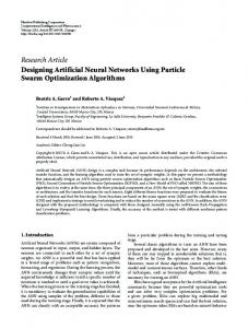
Figure 2: Convergence of PSO on GARP and GIOP PSO is very near this limit and very near the smallest error found. In this protocol, PSO is not able to improve the error trail as much as with GARP. DFS finds an error with length of 2120 transitions, while RandomDFS requires, on average, about 1293 transitions to reach an error. The error trail given by PSO is, again, better for helping the protocol developers to debug it, with only 280 transitions. Regarding the memory required, we can see that DFS and RandomDFS require much less memory than PSO that, as explained before, uses all the available memory as cache. Before concluding this section we are going to present the evolution of the swarm of PSO during the search. In Figure 2 we plot the fitness value of the best particle in each iteration. The horizontal axis represents the iterations, with the first one in the left and the last one in the right. The vertical axis represents the fitness value. For each iteration we take the gBest fitness values at that iteration in each of the 50 runs and plot their average. We want to illustrate with this analysis how the convergence of PSO takes place in both protocols. We can observe in this graph that PSO converged faster on GARP and an error has been always found after 25 iterations (in all the executions). In the GIOP proto-
col the curve is not as steep as in the GARP problem, which is in accordance with the results we observed in Table 3, where the time to the first error is larger than in GARP (Table 2). In any of the protocols we can observe that PSO is guided towards the error, either maintaining the previous result or improving it in each iteration. In the last iterations, we can see that the fitness value has surpassed the 10000 value. According to (3) and the constant values we used for DL, whenever a deadlock is found the fitness value is larger than 10000, since for a deadlock to occur all the existing threads must be blocked, increasing the fitness value. The fact that the average of the 50 runs at the last iterations is larger than 10000 also shows that every run had found an error. In conclusion, we can say that the results presented in this section show that while BFS should give the optimum (shortest) error trail, it cannot be used with complex protocols, since it requires too much memory. DFS also has memory constraints with complex protocols, especially if the error cannot be found in the first transitions, as observed for the GARP. While randomizing the transition order may help DFS, the error trails returned by that search method are still very large and therefore difficult to use for debugging. These experiments show that PSO promises to find good, if not optimum, error trails with a small or no time penalty comparing to DFS. Also, PSO can be used with complex programs without running out of memory, as it does not need to store the previously visited states. Storing them can improve performance, which means we can use the available memory for the algorithm’s benefit. 6
Conclusions and Future Work
We have presented here a novel application of the PSO algorithm to find safety errors in network protocols using a model checking based approach. We have implemented and used it with JPF, a model-checker that allows the checking of concurrent programs written in Java, a known language to most developers. To the best of our knowledge, this is the first time that PSO has been applied to find errors in concurrent systems, using either JPF or any other model checker. As future work, we believe it would be interesting to study the influence on the results of some techniques for reducing the amount of memory required in the PSO algorithm, such as partial order reduction or symmetry reduction. It would be interesting to investigate if the results of PSO can be improved using some more recent changes to the basic PSO algorithm, like Fuzzy Adaptive PSO (Shi et al., 2001) or different topologies of the PSO particle neighbourhood against the gBest topology we used in our implementation. It would be also interesting to compare PSO against other metaheuristic searches in the protocol validation problem, like Genetic Algorithms. Finally, some other heuristics could be used in the fitness function of the PSO to check if the error trail or the processing time could be improved.
7
Acknowledgments
This work has been partially funded by the Spanish Ministry of Education and Science and FEDER under contract TIN2005-08818-C04-01 (the OPLINK project), and also by European CELTIC through the Spanish Ministry of Industry funds from FIT-330225-2007-1 (the CARLINK project). REFERENCES Alba, E. and Chicano, F. (2007). Finding safety errors with ACO. In Genetic and Evolutionary Computation Conference, pages 1066–1073, London, UK. ACM Press. Ammann, P., Black, P., and Majurski, W. (1998). Using model checking to generate tests from specifications. In Proceedings of the 2nd IEEE International Conference on Formal Engineering Methods, pages 46–54, Brisbane, Australia. IEEE Computer Society Press. Blum, C. and Roli, A. (2003). Metaheuristics in combinatorial optimization: Overview and conceptual comparison. ACM Computing Surveys, 35(3):268–308. Burch, J. R., Clarke, E. M., Long, D. E., McMillan, K. L., and Dill, D. L. (1994). Symbolic model checking for sequential circuit verification. IEEE Transactions on Computer-Aided Design of Integrated Circuits and Systems, 13(4). Clarke, E., Grumberg, O., Minea, M., and Peled, D. (1999). State space reduction using partial order techniques. International Journal on Software Tools for Technology Transfer (STTT), 2(3):279–287. Clarke, E. M. and Emerson, E. A. (1982). Design and synthesis of synchronization skeletons using branching-time temporal logic. In Logic of Programs, Workshop, pages 52–71, London, UK. Springer-Verlag. Clarke, E. M., Emerson, E. A., and Sistla, A. P. (1986). Automatic verification of finite-state concurrent systems using temporal logic specifications. ACM Trans. Program. Lang. Syst., 8(2):244–263. Clarke, E. M., Grumberg, O., and Peled, D. A. (2000). Model Checking. The MIT Press. Edelkamp, S., Leue, S., and Lluch-Lafuente, A. (2004). Directed explicit-state model checking in the validation of communication protocols. International Journal of Software Tools for Technology Transfer, 5:247–267. Godefroid, P. and Khurshid, S. (2004). Exploring very large state spaces using genetic algorithms. International Journal on Software Tools for Technology Transfer, 6(2):117–127. Groce, A. and Visser, W. (2004). Heuristics for model checking Java programs. International Journal on Software Tools for Technology Transfer (STTT), 6(4):260–276. Holzmann, G. J. (2004). The SPIN Model Checker. AddisonWesley. Holzmann, G. J., Peled, D., and Yannakakis, M. (1996). On nested depth first search. In Proceedings of the Second SPIN Workshop, pages 23–32. American Mathematical Society.
Kamel, M. and Leue, S. (1998). Validation of the general interorb protocol (giop) using the spin model-checker. Technical report, Department of Electrical and Computer Engineering University of Waterloo. Kennedy, J. and Eberhart, R. (1995). Particle swarm optimization. In IEEE International Conference on Neural Networks, volume 4. Lafuente, A. L. (2003). Symmetry Reduction and Heuristic Search for Error Detection in Model Checking. In Workshop on Model Checking and Artificial Intelligence. Michael, C. C., McGraw, G., and Schatz, M. A. (2001). Generating software test data by evolution. IEEE Transactions on Software Engineering, 27(12):1085–1110. Nakatani, T. (1997). Verification of a group address registration protocol using promela and spin. Shi, Y. and Eberhart, R. (1998). Parameter selection in particle swarm optimization. Evolutionary Programming, 7:611– 616. Shi, Y., Eberhart, R., Team, E., and Kokomo, I. (2001). Fuzzy adaptive particle swarm optimization. In Congress on Evolutionary Computation, volume 1. Valmari, A. (1998). Lectures on Petri Nets I: Basic Models, volume 1491 of Lecture Notes in Computer Science, chapter The state explosion problem, pages 429–528. Springer.
AUTHOR BIOGRAPHIES MARCO FERREIRA is professor in the Escola Superior de Tecnologia e Gest˜ao de Leiria, Pertugal. Nowadays he is a PhD student in the University of Extremadura. His main research interests is the application of metaheuristic algorithms to model checking. FRANCISCO CHICANO is assistant professor in the University of M´alaga, Spain. He received the PhD degree in Computer Science from the same university in 2007. His main research lines include the application of metaheuristic algorithms to optimization problems and, in particular, to Software Engineering problems. His Web-page can be found at neo.lcc.uma.es/staff/francis. ENRIQUE ALBA is tenure in the University of M´alaga, Spain. He received the PhD degree in Computer Science from the same university in 1999. His main research lines focus on metaheuristic algorithms in general. His Webpage can be found at www.lcc.uma.es/˜eat. JUAN A. GOMEZ-PULIDO is professor in the University of Extremadura, Spain. He received the PhD degree in Computer Science from the Complutense University of Madrid in 1993. His main research interests are applications of reconfigurable hardware to accelerate evolutionary algorithms used in optimization problems. His Web-page can be found at arco.unex.es/jangomez.